Label Noise Cleaning Using Support Vector Machines

(1)

University of South Florida

Scholar Commons

Graduate Theses and Dissertations

Graduate School

2-11-2016

Label Noise Cleaning Using Support Vector

Machines

Rajmadhan Ekambaram

University of South Florida, [email protected]

Follow this and additional works at:

http://scholarcommons.usf.edu/etd

Part of the

Computer Sciences Commons

Scholar Commons Citation

Ekambaram, Rajmadhan, "Label Noise Cleaning Using Support Vector Machines" (2016).Graduate Theses and Dissertations.

(2)

Label Noise Cleaning Using Support Vector Machines

by

Rajmadhan Ekambaram

A thesis submitted in partial fulfillment of the requirements for the degree of Master of Science in Computer Science Department of Computer Science and Engineering

College of Engineering University of South Florida

Major Professor: Lawrence Hall, Ph.D. Rangachar Kasturi, Ph.D.

Dmitry Goldgof, Ph.D.

Date of Approval: February 9, 2016

Keywords: Mislabeled Examples, SVM

(3)

DEDICATION

I dedicate this MS. to Dr. Surendra Ranganath. He was my master’s project adviser and mentor at NUS. He provided me the opportunity to learn about this fascinating field of computer vision

and machine learning. His teaching style instilled me the interest in pattern recognition. His mentoring helped me to complete my master’s project at NUS and pursue Ph.D. in computer

(4)

ACKNOWLEDGMENTS

I would like to thank Dr. Lawrence Hall, Dr. Dmitry Goldgof and Dr. Rangachar Kasturi for proving me the opportunity to work on this project. I particularly thank Dr. Lawrence Hall for spending time with all the discussion about the experiments, and in reviewing the paper drafts and this Thesis and providing critical comments. Without his help this work would have not been completed. I also thank Dr. Sergiy Fefilatyev, Dr. Matthew Shreve and Dr. Kurt Kramer for helping with the experiments and in reviewing the paper published through this work. I also thank the research computing team at USF for helping me run the experiments efficiently.

(5)

TABLE OF CONTENTS

LIST OF TABLES . . . iii

LIST OF FIGURES . . . iv ABSTRACT . . . v CHAPTER 1 : INTRODUCTION . . . 1 1.1 Motivation . . . 1 1.2 Contributions . . . 3 1.3 Thesis Overview . . . 4 CHAPTER 2 : BACKGROUND . . . 5 2.1 Introduction . . . 5 2.2 Related Work . . . 8

2.2.1 Weight or Confidence Based Measures . . . 9

2.2.2 Approaches Exploiting the Classifier’s Properties . . . 11

2.2.3 Mitigation of the Effects of the Label Noise Examples on to the Classifier 12 2.2.4 Outliers Detection Using OCSVM . . . 13

2.2.5 Comparing to a Probabilistic Approach . . . 13

2.3 Conclusions . . . 14

CHAPTER 3 : LABEL NOISE REDUCTION USING SVM . . . 15

3.1 Introduction . . . 15

3.2 Experimental Setup . . . 15

3.2.1 Datasets . . . 15

3.2.2 Features . . . 16

3.2.3 Experimental Protocol . . . 17

3.2.3.1 OCSVM Example Selection . . . 17

3.2.3.2 TCSVM Example Selection . . . 18

3.2.3.3 SVM Classifier Parameter Selection. . . 20

3.3 Results . . . 20

3.4 Conclusions . . . 23

CHAPTER 4 : ACTIVE LABEL NOISE CLEANING . . . 25

4.1 Introduction . . . 25

4.2 Experimental Setup . . . 26

4.2.1 Datasets . . . 26

4.2.2 Features . . . 27

(6)

4.3 Results . . . 31

4.3.1 Computation of Performance Values in the Tables and Graphs . . . 32

4.3.2 Noise Removal Performance of ALNR . . . 36

4.3.3 Performance Comparison of ALNR and ICCN_SMO. . . 37

4.3.3.1 Noise Removal Performance . . . 37

4.3.3.2 Classifier Performance . . . 38 4.3.3.3 Parameter Selection . . . 38 4.3.4 Computational Complexity . . . 38 4.4 Conclusions . . . 39 CHAPTER 5 : CONCLUSIONS . . . 48 REFERENCES . . . 50

(7)

LIST OF TABLES

Table 3.1 Algorithm to verify the hypothesis that the label noise examples are captured in the support vectors . . . 16 Table 3.2 Algorithm to find the label noise examples with One-class SVM classifier. . . 18 Table 3.3 The number of examples used in each of the experiments at 10% the noise level . . . . 19 Table 3.4 The result of a single run of experiment 4 with an OCSVM classifier on the MNIST

data at the 10% noise level . . . 21 Table 3.5 The result of a single run of experiment 4 with a TCSVM classifier on the MNIST

data at 10% noise level . . . 21 Table 3.6 The average performance over 180 experiments on both the MNIST and UCI data

sets and the overall performance at the 10% noise level . . . 22 Table 3.7 The average performance of OCSVM with RBF kernel for different “µ” values over

180 experiments on both the MNIST and UCI data set at the 10% noise level. . . 23 Table 4.1 The proposed algorithm to efficiently target the label noise examples in the support

vectors . . . 26 Table 4.2 The number of examples used in each of the experiments at 10% noise level . . . 30 Table 4.3 The average performance of ALNR in selecting the label noise examples for labeling

over 240 experiments on all the data sets for the Random and Default parameter selection experiments . . . 33 Table 4.4 Average noise removal performance of ALNR and ICCN_SMO on all the datasets . 34 Table 4.5 Average examples reviewed for ALNR and ICCN_SMO on all the datasets . . . 35 Table 4.6 Average number of batches required for reviewing the datasets by ALNR and

(8)

LIST OF FIGURES

Figure 2.1 Decision boundary created by a two class SVM classifier . . . 6

Figure 3.1 The sampling process of examples for an experiment . . . 18

Figure 3.2 Example misclassification results . . . 23

Figure 4.1 The sampling process of examples for an experiment . . . 29

Figure 4.2 Performance comparison of ALNR and ICCN_SMO with the Linear Kernel SVM for different parameter selection methods on the UCI Letter recognition dataset . . 40

Figure 4.3 Performance comparison of ALNR and ICCN_SMO with the RBF Kernel SVM for different parameter selection methods on the UCI Letter recognition dataset . . 41

Figure 4.4 Performance comparison of ALNR and ICCN_SMO with the Linear Kernel SVM for different parameter selection methods on the MNIST Digit recognition dataset 42 Figure 4.5 Performance comparison of ALNR and ICCN_SMO with the RBF Kernel SVM for different parameter selection methods on the MNIST Digit dataset . . . 43

Figure 4.6 Performance comparison of ALNR and ICCN_SMO with the Linear Kernel SVM for different parameter selection methods on the Wine Quality dataset . . . 44

Figure 4.7 Performance comparison of ALNR and ICCN_SMO with the RBF Kernel SVM for different parameter selection methods on the Wine Quality dataset . . . 45

Figure 4.8 Performance comparison of ALNR and ICCN_SMO with the linear kernel SVM for different parameter selection methods on the Breast cancer dataset . . . 46

Figure 4.9 Performance comparison of ALNR and ICCN_SMO with the RBF Kernel SVM for different parameter selection methods on the Breast cancer dataset . . . 47

(9)

ABSTRACT

Mislabeled examples affect the performance of supervised learning algorithms. Two novel approaches to this problem are presented in this Thesis. Both methods build on the hypothesis that the large margin and the soft margin principles of support vector machines provide the characteristics to select mislabeled examples. Extensive experimental results on several datasets support this hypothesis. The support vectors of the one-class and two-class SVM classifiers captures around 85% and 99% of the randomly generated label noise examples (10% of the training data) on two character recognition datasets. The numbers of examples that need to be reviewed can be reduced by creating a two-class SVM classifier with the non-support vector examples, and then by only reviewing the support vector examples based on their classification score from the classifier. Experimental results on four datasets show that this method removes around 95% of the mislabeled examples by reviewing only around about 14% of the training data. The parameter independence of this method is also verified through the experiments. All the experimental results show that most of the label noise examples can be removed by (re-)examining the selective support vector examples. This property can be very useful while building large labeled datasets.

(10)

CHAPTER 1 : INTRODUCTION1

1.1 Motivation

The deepwater horizon oil created an interesting problem for computer vision and machine learning scientists which involved finding ways to separate the oil-droplets and plankton from the images captured with the SIPPER platform [1]. A Plankton and other objects dataset was created to explore machine learning solutions to this problem. The plankton dataset had 36 classes and consists of examples belonging to the classes: planktons (32 classes), air bubbles, oil droplets/suspected fish eggs and noise. There were about 8537 examples in this dataset, which is just 0.5% of all the collected SIPPER images. The dataset was labeled by marine science experts based on visual analysis. Originally, small particles were labeled oil droplets. Later, NOAA asked that they be labeled fish eggs. In any event, it was desired to get their labels correct and that was non-trivial. During this labeling process several of the suspected fish eggs were mislabeled, mainly because it is a new class, as air bubbles and to some other classes in the dataset. One solution to correct the mislabeled examples is to manually relabel all the examples. This process will be laborious and requires the precious time of the marine science experts. A better solution will be to sample a small subset of potentially mislabeled examples and produce only these examples to the experts for review. This solution will act as a trade-off between amount of noise that gets removed from the 1_{Portions of this chapter were reprinted from Pattern Recognition, 51, Ekambaram, R., Fefilatyev, S., Shreve, M.,}

Kramer, K., Hall, L. O., Goldgof, D. B., & Kasturi, Active cleaning of label noise, 463-480 Copyright (2016), with permission from Elsevier

(11)

dataset and the time and effort of the experts. This latter approach forms the basis of the problem for this thesis.

Mislabeled examples in the training data affects the learning algorithm, typically, with negative consequences. It has been theoretically shown that label noise examples (i.e., mislabeled examples) reduces the classifier performance in the works of [2, 3, 4, 5]. Label noise might also increases the required number of training instances or the complexity of the classifier as shown in the works of [6, 7]. Other effects include the change in frequency of the class examples which might be problematic in medical applications, poor estimation of performance of the classifiers, decrease in the importance of some features and poor feature selection and ranking. Several approaches have been proposed in the literature [8, 9, 10, 11, 12, 13, 14, 15, 16, 17, 18, 19, 20] to address this critical problem. Though some of the approaches, for examples the methods proposed in [18, 19, 20, 10], uses support vector machine (SVM) classifiers, none of them focuses solely on the support vectors. The method in [21] showed that the SVM classifier has the property to capture mislabeled examples as its support vectors. The hypothesis is that the mislabeled examples tend to be on the margin and get chosen as support vectors of the SVM classifier. Another novel method which builds on this hypothesis was developed in the work of [22]. These two methods are explained in detail in this thesis and validated with extensive experimental results.

The noise removal performance of both a one-class SVM (OCSVM) and two-class SVM (TCSVM) classifiers are analyzed in Chapter 3. Reviewing just the support vectors of the OCCSVM and TCSVM classifier results in the removal of around 85% and 99% of the label noise examples respectively when the amount of mislabeled examples is 10%. For the OCSVM classifier it requires

(12)

Though both OCSVM and TCSVM remove majority of the label noise examples, the amount of examples to be reviewed is high.

The other method presented in Chapter 4 reduces the number of examples needed for review. This method proposed in [10], shows that reviewing examples in decreasing order of probability of the SVM classifier removes label noise examples and results in reviewing fewer examples. But the method has the following problems: 1) dependency on classifier parameters, 2) the need for the selection of the number of examples to review in each batch, and 3) the need for a threshold to stop the review process. Inspired by this approach and to overcome the above mentioned problems a new method is proposed in Chapter 4. The new method assumes that a relatively noise free classifier can be used to target the label noise examples. The method in Chapter 3 shows that most of the label noise examples are selected as support vectors, so the classifier built with non-support vector examples is relatively noise free. The label noise examples in the support vectors can be targeted with this relatively noise free classifier. This approach leads to a significant reduction in the number of examples to be reviewed to remove the mislabeled examples.

1.2 Contributions

My contributions in this thesis are described below.

1. Experimental validation of the effectiveness of 2-SVM to capture the label noise examples as support vectors.

2. Experimental comparison of 1-class SVM, 2-class SVM and their combination to find the label noise examples.

(13)

1.3 Thesis Overview

Chapter 2 describes the SVM optimization problem and the prior works in the literature that deal with finding and removing label noise examples in the labeled datasets.

Chapter 3 demonstrates the hypothesis that label noise examples are captured as the support vectors of the SVM by experiments. Three different experiments using 1-class SVM, 2-class SVM and their combination were conducted to evaluate the hypothesis and to compare their performances.

Chapter 4 describes a novel method that builds on SVM and analyzes its performance by experiments. Performance comparison with a more closely related method in the literature is also shown.

Chapter 5 presents the conclusion and potential future works that can be done to improve the performance of the proposed methods and the other methods that could be tried.

(14)

CHAPTER 2 : BACKGROUND2

2.1 Introduction

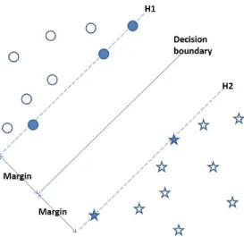
Support vector machines (SVM) are a class of algorithms that are used for classification and regression tasks. Only SVM classification algorithm is dealt with this thesis. SVM is a discriminative classifier, in which the prediction is done by finding a separating hyperplane between the examples from two classes. The hyperplane is found based on the principle of maximum margin. In a linear classifier the distance between the separating hyperplane and an example is called the margin. In SVM, maximizing this margin involves finding the direction that increases the distance between the two or more closest examples (at least one from each class). A classification based on the maximum margin principle is shown in Figure 2.1.

The hyperplanes in the example shown in Figure 2.1 are described by the following equations:

~ w·x~i−b≥+1, if y~i= +1 and ~ w·x~i−b≤ −1, if y~i=−1 (2.1)

wherew~ is the normal vector to the hyperplane,x~i are the training examples, andyi ∈[−1,+1]are

the class labels. The distance between these two hyperplanes is given by _w2_~. In order to increase 2_{Portions of this chapter were reprinted from Pattern Recognition, 51, Ekambaram, R., Fefilatyev, S., Shreve, M.,}

Kramer, K., Hall, L. O., Goldgof, D. B., & Kasturi, Active cleaning of label noise, 463-480 Copyright (2016), with permission from Elsevier

(15)

Figure 2.1: Decision boundary created by a two class SVM classifier

the distance between the hyperplanes, kw~k should be reduced.

The equation given in 2.1 for the hyperplanes and the condition on the normal vector can be combined together and written as the following optimization problem:

minimize w ~ kwk subject to y~i(w~ ·x~i−b)≥+1; i= 1, . . . , N. (2.2)

where N is the total number of examples in the dataset.

The solution to this optimization problem only involves the examples that satisfy the condi-tionw~·x~i−b= +1when the class label is +1 orw~·x~i−b=−1when the class label is -1. These are

the examples that affect the solution are called the support vectors. The solution for the equation 2.2 exists only if the examples from the two classes are linearly separable or all the examples in the dataset satisfy the equation 2.1.

(16)

In this method a penalty term (ξ)is added to the optimization equation. The examples which are on the wrong side of the hyperplane are penalized by their distance from the hyperplane. The hyperplanes for this formulation are described by the following equations:

~ w·x~i−b≥+1 +ξi, if y~i= +1 and ~ w·x~i−b≤ −1 +ξi, if y~i=−1 where, ξi ≥0,∀i (2.3)

wherew~ is the normal vector to the hyperplane, x~i are the training examples, and yi ∈[−1,1]are

the class labels. The distance between these two hyperplanes is given by _w2_~. In order to increase the distance between the hyperplanes, kw~k should be reduced.

Though the above equations only results in linear hyperplane, it is possible to create a non-linear decision boundary by simply mapping the input data non-non-linearly in to some high dimensional space using kernel functions. There are two ways to solve the SVM optimization problem: primal and dual. The dual formulation proposed in [24] is efficient for high dimensional features and for applying the “kernel trick” to the features. The SMO-type algorithms described in [25, 26] are an efficient way to compute the support vectors and they solve the dual optimization problem. The dual formulation is 1 2 N X i=1 N X j=1 yiyjK(xi,xj)αiαj−min α N X i=1 αi, (2.4)

(17)

example,K(·)is the kernel andαiis a Lagrange multiplier. Equation 2.4 is subject to two constraints αi ≥0,∀i, (2.5) N X i=1 yiαi = 0. (2.6)

The examples for which αi > 0 are selected as support vectors to create the decision boundary.

These are the examples that our approach selects as the candidates for relabeling. The next section discusses the commonality and the differences between our approach and the other approaches proposed in the literature.

2.2 Related Work

Many approaches are proposed in the literature to identify and remove mislabeled (label noise) examples. Some of these approaches are compared to the proposed approach in this thesis based on three broad ideas:

1. Weight or confidence based measures

2. Approaches exploiting the classifier’s properties

3. Mitigation of the effects of the label noise examples on to the classifier

(18)

2.2.1 Weight or Confidence Based Measures

The method proposed in [8] finds mislabeled examples based on the information gain criteria. An example is considered more informative if it is difficult to predict by the classifier. The prediction is based on the probability of the classification using Shannon’s information gain. The examples which had more information gain were more important for the classifier. So the examples are reviewed based on the decreasing order of their information gain. Our method differs from the method in [8] in the following ways:

• the strict use of a human in the loop

• how the examples are ranked

• how to find the number of rounds

• stopping criteria for the review

The method proposed in Rebbapragada et al. [9] selects the potential examples for relabeling using an SVM classifier in an active learning framework. The unlabeled examples which lie close to the separating hyperplane were selected for labeling. The intuition for our method is similar to this method. The differences are the following:

• All the examples in our method are labeled

• Only support vectors are examined in our method. The examples selected in this method may or may not become support vectors.

The method proposed in Rebbapragada [10] and Brodley et al. [27] uses an SVM classifier to find the label noise examples. Both of these methods review the examples in decreasing order

(19)

of probability of classification [28] returned by the SVM classifier. The selected examples in these methods are not necessarily support vectors. Depending on the threshold used for selection, exam-ples which are on the wrong side of the boundary may be ignored. A detailed comparison of this method is described in section 2.2.5.

The method proposed in Gamberger et al. [11] assigns a weight for the examples based on the complexity measure of the classifier. The example with the highest weight is selected for review if its weight exceeds the threshold. The number of rounds in this method equals the number of label noise examples expected in the dataset and this method requires a threshold.

A confidence based method was proposed in Rebbapragada and Brodley [16] and Rebbapra-gada et al. [17]. Examples are clustered pair wise and a confidence is assigned to each example based on the Pair Wise Expectation Maximization (PWEM) method. This method generates confidence measure based on PWEM and our method can generate probabilities based on the distance from the hyperplane.

A distributed rule based method similar to the method in [12] was proposed in Zhu et al. [13]. This method distinguishes between exceptions and mislabeled examples. This method assumes that the mislabeled examples will be classified wrongly by more rules than the exception examples. The distributed dataset was divided into subsets and rules were generated for all the subsets. The examples were classified using all the generated rules. Exceptions are not handled in our method and it can work in a distributed system provided sufficient positive and negative examples are present in each location.

(20)

2.2.2 Approaches Exploiting the Classifier’s Properties

Local geometrical structure is used to find the mislabeled examples in the method proposed in Muhlenbach et al. [14]. An example is chosen as a potential mislabeled examples based on its neighborhood in the Relative Neighborhood graph. If an example has more connection with the opposite class than the global proportion of examples belonging to its current class, then it is a candidate for the mislabeled example. The similarity between this method and our method is that both suspects the closest examples from the other classes. The dissimilarity is that our method considers all the examples in the dataset at the same time, whereas this method considers only the local examples.

A weighted k nearest neighbors (kNN) approach was extended to a quadratic optimization problem in the method proposed in Valizadegan and Tan [15]. The optimization expression depends only on the similarity between the examples, so a kernel based solution was proposed. This results in solving the problem easily by projecting the attributes into higher dimensions with the help of a kernel. The suspected mislabeled examples are the ones whose label switching maximizes the optimization expression. Both the methods use an optimization function, but the objective of the optimization function is different.

An automatic noise removal method was proposed in Brodley and Friedl [12]. The primary intention behind this method was to improve the classifier accuracy. So this method removes the good examples and may miss some mislabeled examples. This method might not suitable for classes with a small number of examples.

(21)

2.2.3 Mitigation of the Effects of the Label Noise Examples on to the Classifier

Our proposed method applies only for removing the label noise examples in the training data, and though the final noise reduced SVM classifier can be directly used in the application, it is not the focus of our method. The methods discussed in this section both handle noise and create classifiers in a single step.

AdaBoost tends to overfit in the presence of label noise examples as was shown in Ratsch et al. [29] and Dietterich [30]. To reduce the bias due to mislabeled examples, a method was proposed in Cao et al. [31], that reduces the weights of the mislabeled examples using kNN and Expectation Maximization methods.

An SVM based label noise mitigation approach was presented in Biggio et al. [18], Stempfel and Ralaivola [19] and Niaf et al. [20]. The SVM problem formulation was modified to handle the label noise problem. The method proposed in Biggio et al. [18] reduces the effect of any single example on the decision boundary by modifying the kernel matrix of the SVM. The modified kernel matrix will result in more support vectors and hence reduces the influence of the potential label noise examples in the dataset.

The method proposed in [19] estimates the noise free slack variables from the noisy data. The noise-free SVM objective function is the mean of the newly defined non-convex objective function.

Another SVM based approach is proposed in [20]. The noise is controlled using the slack variable in the SVM problem formulation based on the probability of the examples generated using Platt’s scaling algorithm [28].

(22)

2.2.4 Outliers Detection Using OCSVM

The method proposed in Schölkopf et al. [32] extends the maximum margin principle to examples from only one class. The method is referred to as a one-class SVM (OCSVM). Similar to clustering, this method finds a small region that encloses the data, and classifies the examples that are in the boundary of the region as outliers. Several works in the literature use this method to find the outliers in a dataset. A few of those methods are:

• A method for cleaning images belonging to different categories namely Snow and Skiing, Family and Friends, Architecture and Buildings and Beach was proposed in Lukashevich et al. [33]

• A method for cleaning satellite images in a distributed framework was proposed in [34]

• A method to find depressed patients using fMRI response was proposed in [35]

In our work the examples which are detected as outliers by the OCSVM are considered as suspected label noise examples.

2.2.5 Comparing to a Probabilistic Approach

A method very close in principle to our method was proposed in [10]. In this work several methods were proposed (SMO, Logistic Regression, Boosting, Bagging, Nearest neighbor and Naive Bayes) for Iterative Correction of Class Noise (ICCN) and their performance was compared for finding the label noise examples. The SMO confidence based method in this work is similar to our method and is one of the best performing methods. The examples were sorted based on their probability of classification and reviewed in batches. Twenty examples with the least probability of

(23)

classification were reviewed in each batch. The stopping criteria is decided by the reviewer. In the reported experiments the review was stopped when the total number of reviewed examples equaled the total number of mislabeled examples in the dataset. Some important difference between this method and our approach are as follows:

• This method does not differentiate between the support vector examples and the non-support vector examples, and reviews all the examples based on their probability of classification. Only the subset consisting of support vector examples are reviewed in our method.

• Examples are selected based on a two stage process in our method

• Our method does not have a threshold parameter for the number of examples to be reviewed in a batch

• Our method has a clear stopping point, but this method does not. Stopping criteria is useful when the amount of label noise in the data is unknown. In data undergoing a real-time labeling process, it is highly likely that the amount of mislabels will be unknown.

2.3 Conclusions

The general principle behind the SVM classifier was introduced in this chapter. The works in the literature which are close in principle to the proposed method were briefly described. The differences between the methods in the literature and the proposed method were also described. A detailed comparison of a very similar SMO based method proposed in [10] was done in this chapter.

(24)

CHAPTER 3 : LABEL NOISE REDUCTION USING SVM3

3.1 Introduction

This chapter describes the algorithm to find and remove the label noise examples in the labeled datasets. The method is based on the assumption that the large margin and soft margin principles of the SVM have the property of selecting the label noise examples as its support vectors. The label noise examples are more likely to be the border line examples due to the confusion they create for the labeler. It is intuitive to think that the border line examples of the two classes lie close together. The large margin principle is to increase the distance between the two classes, which results in selecting the examples from the two classes that are close together as support vectors. Hence it is more likely that these border line examples are selected as Support vectors. These are the borderline examples which are selected by our algorithm for review. The algorithm is described in Table 3.1.

3.2 Experimental Setup

3.2.1 Datasets

The potential of this method was tested with two datasets widely used in the machine learning community:

3

Portions of this chapter were reprinted from Pattern Recognition, 51, Ekambaram, R., Fefilatyev, S., Shreve, M., Kramer, K., Hall, L. O., Goldgof, D. B., & Kasturi, Active cleaning of label noise, 463-480 Copyright (2016), with permission from Elsevier

(25)

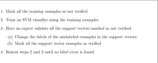
Table 3.1: Algorithm to verify the hypothesis that the label noise examples are captured in the support vectors.

1. Mark all the training examples as not verified 2. Train an SVM classifier using the training examples

3. Have an expert validate all the support vectors marked as not verified: (a) Change the labels of the mislabeled examples in the support vectors (b) Mark all the support vector examples as verified

4. Repeat steps 2 and 3 until no label error is found

1. UCI Letter recognition dataset

2. MNIST digit dataset

UCI letter recognition dataset was obtained from the UCI Machine learning repository (http:// archive.ics.uci.edu/ ml) and the MNIST digits dataset was obtained from http:// yann. lecun.com/ exdb/ mnist/. The UCI letter recognition dataset consists of images of 26 printed letters in the English language alphabet. The dataset has around 700 examples for each letter based on 20 different fonts. The MNIST digit recognition dataset consists of images of 10 handwritten digits. The dataset has around 6000 examples for each digit.

3.2.2 Features

Each example in the UCI Letter recognition dataset is represented by a 16 dimensional feature vector. The features capture the statistical moments and edge counts in the images. The

(26)

is represented by a 784 dimensional feature vector. The features are the gray scale pixel values of the digit images.

3.2.3 Experimental Protocol

Performing experiments with all the classes (letters and digits) in both the datasets is tedious. Random selection of the classes might result in selecting classes that are easily separable. So some exploratory experiments were performed for the UCI letter recognition dataset and three letters (H, B and R) which are the most likely to be confused were selected. For the MNIST digits recognition dataset the three digits 4, 7 and 9 were selected. These three digits had the most confusion among them as stated in [36].

All the experiments were performed using the scikit-learn python machine learning library ([37]). scikit-learn uses the LIBSVM library [38] which implements the SMO-type optimization algorithm for SVM classification.

3.2.3.1 OCSVM Example Selection

For the OCSVM experiments with the UCI Letter dataset the training examples for a sample experiment were selected as follows: 450 examples were randomly selected from one of the three letters and 50 examples were randomly selected from the other two letters (25 examples each). The procedure described in Table 3.2 was followed to evaluate the performance of the OCSVM classifier using these training examples. The experiment was repeated 90 times with a different random selection of examples. The number of experiments was distributed evenly between all the letters. A similar procedure was followed for the MNIST digit dataset. The MNIST dataset contains more examples for each digit, so more examples are used in each experiment. For each experiment

(27)

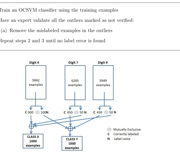
900 examples were randomly selected from one of the three digits and 100 examples were randomly selected from the other two digits (50 examples each). Figure 3.1 shows how the digits were sampled. Only the examples from Class X as shown in the Figure 3.1 were used with the OCSVM classifier.

Table 3.2: Algorithm to find the label noise examples with One-class SVM classifier.

1. Train an OCSVM classifier using the training examples

2. Have an expert validate all the outliers marked as not verified: (a) Remove the mislabeled examples in the outliers

3. Repeat steps 2 and 3 until no label error is found

Figure 3.1: The sampling process of examples for an experiment

(28)

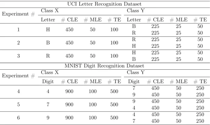
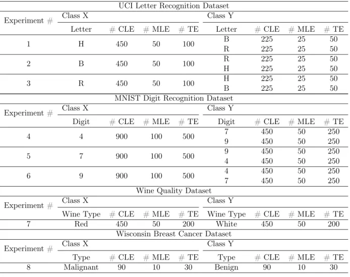
Table 3.3: The number of examples used in each of the experiments at 10% the noise level. CLE - correctly labeled examples, MLE - mislabeled examples, TE - test examples. The number of examples correspond to the letter or digit or wine type in the same row under the same class. The mislabeled examples in Class X are labeled as Class Y and vice-versa.

UCI Letter Recognition Dataset

Experiment # Class X Class Y

Letter # CLE # MLE # TE Letter # CLE # MLE # TE

1 H 450 50 100 B 225 25 50 R 225 25 50 2 B 450 50 100 R 225 25 50 H 225 25 50 3 R 450 50 100 H 225 25 50 B 225 25 50

MNIST Digit Recognition Dataset

Digit # CLE # MLE # TE Digit # CLE # MLE # TE

4 4 900 100 500 7 450 50 250 9 450 50 250 5 7 900 100 500 9 450 50 250 4 450 50 250 6 9 900 100 500 4 450 50 250 7 450 50 250

letters, 500 examples each. Out of the 500 selected examples from each letter 50 of them were ran-domly selected and mislabeled. Then the procedure described in Table 3.1 was followed to evaluate the performance of the TCSVM classifier using these training examples. Similar to the OCSVM experiments, 90 runs of this experiment each with a different sampled examples was repeated, evenly distributing the number of experiments between all three letters. A similar procedure was followed for the MNIST digit dataset. For each MNIST experiment 2000 examples were randomly selected from two of the three letters, 1000 examples each. Out of the 1000 selected examples from each letter 100 of them were randomly selected and mislabeled.

(29)

3.2.3.3 SVM Classifier Parameter Selection

The feature values were scaled in-to the range of values between -1 and 1. Linear and RBF kernels were explored. The parameters “C” and “γ” were chosen using a 5-fold cross validation

method. The SVM cost parameter “C” was varied between 1 and 25 in steps of 3. The RBF

kernel parameter “γ” was varied in multiples of 5 from 0.1/(number of features) to 10/(number of features). In addition, two other “γ” values 0.01/(number of features) and 0.05/(number of features) were tested.

3.3 Results

All the experiments were carried out with 10% label noise examples. To avoid bias all the experiments were repeated 30 times with different random sampling of examples and the average of the results are reported. The detailed sample results of one run of the experiments with OCSVM are shown in Table 3.4 and with TCSVM are shown in Table 3.5. The overall performance is shown in Table 3.6. OCSVM with linear and RBF kernel captured 85.75% and 85.79% of label noise examples respectively as outliers. TCSVM captured 99.55% of label noise examples as its support vectors with both the linear and RBF kernel.

From Tables 3.4 and 3.5 it can observed that the majority of the noise examples were removed in the 1st round of iterations. Very few noise examples were removed in the subsequent rounds in all the experiments. Though Tables 3.4 and 3.5 show the results for one run of the experiments, similar results were observed in all the experiments. From Table 3.6 it can be observed that up-to 45% of the examples can be support vectors when 10% of the examples have incorrect noisy labels.

(30)

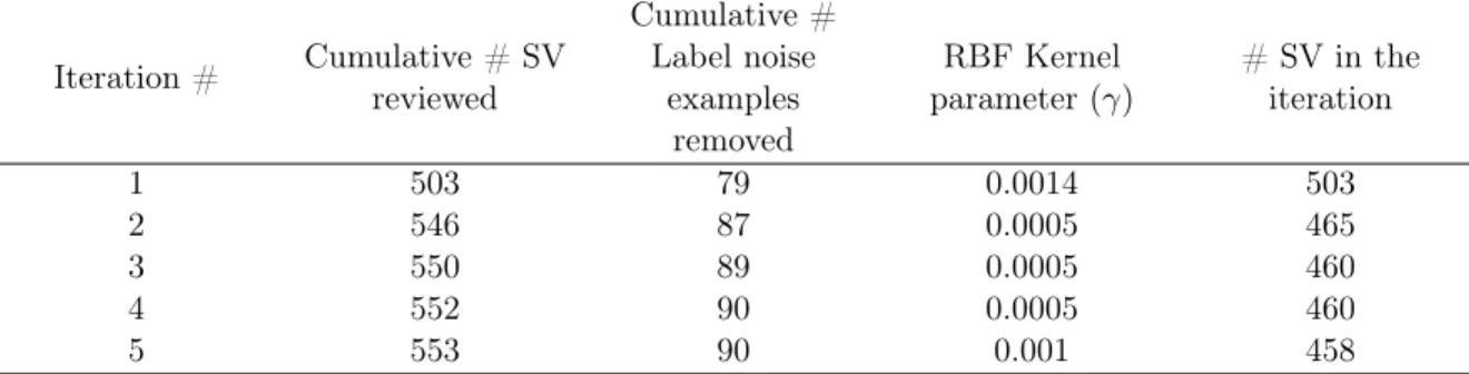
Table 3.4: The result of a single run of experiment 4 with an OCSVM classifier on the MNIST data at the 10% noise level. This table shows the iteration number, the cumulative number of support vectors to be reviewed until that iteration, the cumulative number of label noise examples selected as support vectors until that iteration, the kernel parameters used for that iteration and the number of support vectors selected in that iteration by the OCSVM classifier. The parameter “µ” was set to 0.5. Iteration # Cumulative # SV reviewed Cumulative # Label noise examples removed RBF Kernel parameter (γ) # SV in the iteration 1 503 79 0.0014 503 2 546 87 0.0005 465 3 550 89 0.0005 460 4 552 90 0.0005 460 5 553 90 0.001 458

Table 3.5: The result of a single run of experiment 4 with a TCSVM classifier on the MNIST data at 10% noise level. This table shows the iteration number, the cumulative number of support vectors to be reviewed after that iteration, the cumulative number of label noise examples selected as support vectors until that iteration, the kernel parameters used for that iteration and the training accuracy of the classifier using that kernel parameter in that iteration. In this case all noise examples were removed. # Iteration Cumulative # SV reviewed Cumulative # Label noise examples removed Parameter “ C” RBF Kernel parameter (γ) Training accuracy in % 1 841 199 25 0.001 88.8 2 848 200 22 0.005 98.95 3 849 200 25 0.005 98.75

(31)

support vectors. The number to be looked at may not scale well as the training set becomes large in some cases.

Table 3.6: The average performance over 180 experiments on both the MNIST and UCI data sets and the overall performance at the 10% noise level. For OCSVM these results were obtained when using the value 0.5 for parameter “µ”

Dataset Linear Kernel OCSVM TCSVM Combined % outliers % noise removed % support vectors % noise removed % support vectors % noise removed MNIST 55.05 89.46 42.91 98.23 68.18 99.67 UCI 55.02 78.33 48.80 97.92 69.52 99.31 Overall 55.04 85.75 44.87 98.13 68.63 99.55 Dataset RBF Kernel OCSVM TCSVM Combined % outliers % noise removed % support vectors % noise removed % support vectors % noise removed MNIST 55.23 91.21 45.56 99.85 69.11 99.95 UCI 54.93 74.95 42.80 99.78 68.13 99.95 Overall 55.13 85.79 44.64 99.83 68.78 99.95

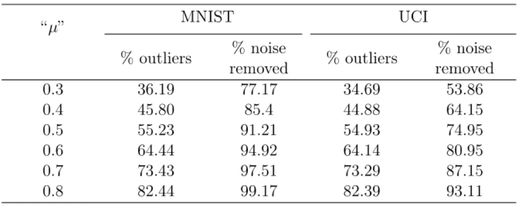
The parameter “µ” was varied between 0.3 and 0.8 to check its effect on the performance of OCSVM. It can be observed from the Table 3.7 that large number of examples need to be reviewed to find the label noise examples. The result is not desirable for large datasets.

Another experiment in which viewing the combination of the support vectors of both

OCSVM and TCSVM was explored. The support vectors of the OCSVM (with “µ” = 0.5) and

TCSVM classifiers (only the support vectors of the class used in OCSVM) at each iteration were added together and examined for the presence of label noise examples. The combination experiment

(32)

than TCSVM for both the linear and RBF kernel respectively. The results of this experiment are shown in Table 3.6.

Table 3.7: The average performance of OCSVM with RBF kernel for different “µ” values over 180 experiments on both the MNIST and UCI data set at the 10% noise level.

“µ” MNIST UCI % outliers % noise removed % outliers % noise removed 0.3 36.19 77.17 34.69 53.86 0.4 45.80 85.4 44.88 64.15 0.5 55.23 91.21 54.93 74.95 0.6 64.44 94.92 64.14 80.95 0.7 73.43 97.51 73.29 87.15 0.8 82.44 99.17 82.39 93.11

Figure 3.2: Example misclassification results. The images on the left and right are labeled as 4 and 9 respectively in the dataset. The image on the left is correctly identified as a mislabeled example, whereas the image on the right is incorrectly identified as a correctly labeled example.

15 label noise examples were missed by the TCSVM with RBF kernel in total over 90 (3 experiments * 30 repetitions) MNIST dataset experiments. Figure 3.2 shows two examples missed by the RBF kernel. The image on the left is mislabeled as a 4 in the dataset and its correct label is 9. The digit in the image is a bit ambiguous and hence it seems to be a reasonable miss by our method. The image on the right is mislabeled as 9 in the dataset and its correct label is 4. The digit 4 appears clear in the image, but our method failed to identify it as a label noise example.

3.4 Conclusions

The experiments described in this chapter show promising results to support the hypothesis that the SVM has the property to capture label noise examples as its support vectors. Both

(33)

OCSVM and TCSVM capture around the 85% and 99% of the label noise examples as its outliers and support vectors respectively by reviewing around 55% and 45% of the examples in the dataset. TCSVM outperforms OCSVM in both the amount of label noise examples removed and the number of examples to be reviewed. Though the computation involved in the combination experiment is high, it shows some improvement in performance.

(34)

CHAPTER 4 : ACTIVE LABEL NOISE CLEANING4

4.1 Introduction

The effectiveness of reviewing only the support vectors to find the label noise examples was demonstrated in Chapter 3. Though the method is effective in finding over 90% of label noise examples the number of examples to be reviewed is around 55% for OCSVM and 44% for TCSVM. Reviewing all these support vector examples for large datasets is a tedious process. This Chapter describes a method that overcomes this problem by reducing the number of examples that need to be reviewed. The method builds on the SVM classifier and is based on the following two assumptions:

1. majority of the label noise examples are selected as support vectors by the SVM classifier.

2. noise free SVM classifier can be used to target the label noise examples.

The first assumption is supported by the results shown in the Chapter 3. The second assumption is supported by the experimental results that are shown later in this chapter. The method is described in Table 4.1. The intuition is that the noiseless model will act as a good candidate for finding the mislabeled examples. The experimental results support this intuition.

4

Portions of this chapter were reprinted from Pattern Recognition, 51, Ekambaram, R., Fefilatyev, S., Shreve, M., Kramer, K., Hall, L. O., Goldgof, D. B., & Kasturi, Active cleaning of label noise, 463-480 Copyright (2016), with permission from Elsevier

(35)

Table 4.1: The proposed algorithm to efficiently target the label noise examples in the support vectors.

1. Create classifier using all the examples in the dataset 2. Separate all the support vector examples from the dataset 3. Create a new classifier using the non-support vector examples

4. Test all the support vectors with this new classifier, and rank the mis-classified support vector examples based on their probability of classification

5. Have an expert validate the unseen support vectors based on their ranking, starting with low probability examples, and change the labels of the mislabeled examples 6. Repeat all the above steps until no mislabeled example is found in Step 5

4.2 Experimental Setup

The experimental results reported in this chapter show the performance and the parameter independence of the method in selecting the subset of label noise examples in the support vectors. The experiments were performed as shown in the algorithm in Table 4.1. A detailed comparison of the proposed method with the closely related method in [10] is reported. The proposed method is referred as ALNR (Active Label Noise Removal) and the method in [10] as ICCN_SMO.

4.2.1 Datasets

The potential of this novel method was tested with four datasets widely used in the machine learning community:

(36)

3. Wine quality dataset

4. Wisconsin Breast cancer dataset

Two datasets not previously used were obtained from UCI Machine learning repository (http:// archive.ics.uci.edu/ ml). Remember the UCI Letter recognition and the MNIST digit are image datasets; whereas the Wine Quality and the Wisconsin Breast Cancer dataset are non-image datasets. Please refer to the experimental setup described in Chapter 3 for the details of the UCI letter recognition and MNIST digit recognition datasets. The wine quality dataset consists of physicochemical properties of the red and white wines. The dataset has around 1100 examples for the red wine class and 3150 examples for the white wine class. The Wisconsin Breast cancer dataset consists of images of fine needle aspirates of the breast mass. The dataset has around 212 examples for the malignant class and 357 examples for the benign class.

4.2.2 Features

Each example in the wine quality dataset is represented by an 11 dimensional feature vector of real numbers. The features capture the physicochemical properties of the wines. The wine quality dataset has 12 features, the 12th feature is the quality score computed using the 11 physicochemical properties. So the 12th feature is ignored in our experiments. Each example in the breast cancer dataset is represented by a 30 dimensional feature vector of real numbers. The features capture the 10 properties of the nuclei in the image. The mean value, largest value and the standard error of all the nuclei for each of the 10 properties are computed for each image.

(37)

4.2.3 Experimental Protocol

Only the TCSVM was explored for the proposed method. Similar to the experiments in Chapter 3, only the most confusing letters (H, B and R) were used from the UCI letter recognition dataset, and the most confusing digits (4, 7 and 9) were used from the MNIST digits recognition dataset. The wine quality and the breast cancer datasets have only two classes, and both of the classes were used.

All the experiments were performed using scikit-learn python machine learning library ([37]). scikit-learn uses the LIBSVM library [38] which implements the SMO-type optimization algorithm for SVM classification.

4.2.3.1 Example Selection

Training examples for the UCI Letter and the MNIST digit datasets were randomly selected following a similar procedure as described in Chapter 3. For the wine quality dataset 1000 examples were randomly selected from two classes, 500 examples each. For the breast cancer dataset 200 examples were randomly selected from two classes, 100 examples each. The amount of label noise in the dataset was varied from 10% to 50% in steps of 10. The number of label noise examples, for example, in the wine quality dataset at 30% label noise is 150 examples each for the red and white wine classes. Testing examples were also randomly selected from the dataset to estimate the performance of the classifier after the removal of the label noise examples. The number of testing examples for all experiments at different noise levels was kept constant and was mutually exclusive of all the training examples. The number of examples for each of the classes at 20% label noise is

(38)

Figure 4.1: The sampling process of examples for an experiment

4.2.3.2 SVM Classifier Parameter Selection

Parameter selection and feature scaling were done similarly to the experiment setup in Chapter 3.2.3.

4.2.3.3 ICCN_SMO

ICCN_SMO is one of the methods proposed in [10] and is closely related to our proposed method. The differences between the actual implementation of ICCN_SMO and our implementation is described here. In ICCN_SMO the examples are reviewed in batches of 20 examples. The review is stopped when the number of reviewed examples equals or exceeds the total number of label noise examples in the dataset. The choice of 20 examples to review in a batch was arbitrary. The number of examples in each of the datasets in our experiments is different. Reviewing only 20 examples in a large dataset like MNIST will result in a large number of batches while small datasets like breast

(39)

Table 4.2: The number of examples used in each of the experiments at 10% noise level. CLE - correctly labeled examples, MLE - mislabeled examples, TE - test examples. The number of examples correspond to the letter or digit or wine type in the same row under the same class. The mislabeled examples in Class X are labeled as Class Y and vice-versa.

UCI Letter Recognition Dataset

Letter # CLE # MLE # TE Letter # CLE # MLE # TE

1 H 450 50 100 B 225 25 50 R 225 25 50 2 B 450 50 100 R 225 25 50 H 225 25 50 3 R 450 50 100 H 225 25 50 B 225 25 50

MNIST Digit Recognition Dataset

Digit # CLE # MLE # TE Digit # CLE # MLE # TE

4 4 900 100 500 7 450 50 250 9 450 50 250 5 7 900 100 500 9 450 50 250 4 450 50 250 6 9 900 100 500 4 450 50 250 7 450 50 250

Wine Quality Dataset

Wine Type # CLE # MLE # TE Wine Type # CLE # MLE # TE

7 Red 450 50 200 White 450 50 200

Wisconsin Breast Cancer Dataset

Type # CLE # MLE # TE Type # CLE # MLE # TE

8 Malignant 90 10 30 Benign 90 10 30

cancer will result in a small number of batches. The number of examples to review was set to 30, 50, 30 and 20 for the UCI letter, MNIST digit, wine quality and breast cancer respectively. These numbers were chosen in proportion to the number of examples in the dataset. Also, the stopping criteria for the review process was extended to between 20 and 25% more examples than the amount of noise in the dataset.

(40)

4.3 Results

Three experiments were carried out to evaluate the parameter dependence of the proposed method:

1. extensive parameter selection

2. default parameter selection

3. random parameter selection

For all the parameter selection methods both the linear and RBF kernels were explored. For the extensive parameter selection method the parameters of the SVM classifiers were selected following a similar approach described in Chapter 3.2.3. For default parameter selection method the linear kernel parameter “C” was set to 1, and for the RBF kernel the parameters “C”, and “gamma” were set to 1 and 1/(number of features). For the random parameter selection method the parameters were uniformly selected from the range of parameter values described in Chapter 3.2.3. The extensive parameter selection method is referred as “Regular”, the random parameter selection method is referred as “Random” and the default parameter selection method is referred as “Default” in all tables and figures.

All the reported results are the average of the 240 experiments (30 experiments with differ-ent random sampling for the eight experimdiffer-ents listed in Table 4.2). The method involves creating intermediate classifiers when examples are reviewed and re-labeled. The accuracy of these interme-diate classifiers are also reported in addition to the label noise removal performance. The parameter selection for these intermediate classifiers was done following the procedure explained in Chapter 3.2.3. Performance estimation for all the intermediate classifiers was done using the same test

(41)

examples in all 30 repetitions of each experiment and the average performance is reported. RBF kernel with its “C”, and “gamma” set to 1 and 1/(number of features) respectively was used to estimate the classification performance. The classification performance is reported at an interval of about 10% of the total label noise examples in the experiment. For example, for the Wine quality dataset with 30% label noise examples, the classification performance was estimated accuracy after reviewing every 30 examples, whereas for the MNIST dataset with 30% label noise examples, the classification performance was estimated after reviewing every 60 examples. The cumulative results of all the parameter selection methods over all the datasets at different noise levels is shown in Table 4.3.

The detailed results of each experiment are shown in Tables 4.4 and 4.5 and in Figures 4.2 to 4.9.

4.3.1 Computation of Performance Values in the Tables and Graphs

The reported values in the Tables 4.3, 4.4 and 4.5 were the average of the final results of all the experiments. Ideally the computation of all the results shown in both the graphs and the tables should follow the same protocol. Each point in the graph should be the average of all the experiments, for example, 90 experiments for UCI and MNIST with linear and RBF kernels. The averages were based on the number of examples reviewed in each experiment. It can easily be understood that in each experiment there would be reviewed a different number of examples. Due to the experimental setting, it is not possible for all the experiment to contribute values for all the points in the graph. If only a few experimental results were available for some portion of

(42)

Table 4.3: The average performance of ALNR in selecting the label noise examples for labeling over 240 experiments on all the data sets for the Random and Default parameter selection experiments.

Extensive parameter selection experiment

% Noise level Linear Kernel RBF Kernel

% examples reviewed % noise removed % examples reviewed % noise removed 10 16.40 93.56 13.34 95.84 20 26.40 93.92 23.47 96.01 30 37.26 93.99 34.08 95.69 40 50.64 94.32 48.20 95.72 50 70.03 94.89 71.11 96.22

Random parameter selection experiment

Default parameter selection experiment

(43)

Table 4.4: Average noise removal performance of ALNR and ICCN_SMO on all the datasets. The performance is the average over 90 experiments on the UCI Letter and MNIST Digits datasets, and 30 experiments on the Wine Quality and Breast cancer datasets. Regular, Random and Default refer to the extensive, random and default parameter selection experiments respectively. All the results are in percentage of noise examples reviewed versus all examples reviewed.

UCI Letter Recognition Dataset Noise Level %

Kernel: Linear Kernel: RBF

Regular Random Default Regular Random Default

ALNR ICCN_SMO ALNR ICCN_SMO ALNR ICCN_SMO ALNR ICCN_SMO ALNR ICCN_SMO ALNR ICCN_SMO

10 90.48 78.18 90.91 78.07 90.04 77.84 95.09 93.14 94.50 89.54 88.02 80.71

20 90.77 86.92 91.44 86.88 90.50 86.79 95.39 94.55 94.87 91.33 88.38 88.07

30 90.80 90.98 91.40 91.02 90.53 90.97 94.39 95.42 94.56 93.34 87.98 91.58

40 91.02 93.20 90.94 93.24 90.74 93.25 93.80 95.87 94.69 91.88 87.76 93.65

50 92.09 39.42 92.25 38.17 91.98 35.48 92.98 55.96 93.74 46.80 82.08 34.26

MNIST Digit Recognition Dataset Noise Level %

10 94.08 70.82 94.25 59.01 94.07 71.38 95.75 86.69 96.36 78.16 94.12 93.88

20 94.63 77.65 94.75 68.85 94.59 78.60 95.91 90.47 96.62 85.33 94.10 96.65

30 94.69 81.55 94.55 74.64 94.66 82.49 95.80 86.68 96.72 87.86 94.09 97.84

40 95.12 75.57 95.14 70.58 95.12 81.54 96.15 81.91 96.79 87.84 94.32 98.58

50 95.49 67.90 95.68 65.56 95.49 72.39 97.33 43.45 97.70 53.05 95.90 35.22

Wine Quality Dataset Noise Level %

10 99.17 99.37 99.23 99.33 99.17 99.47 99.00 98.73 99.10 98.30 98.93 99.37

20 98.77 99.33 98.87 99.28 98.75 99.30 98.72 99.13 98.78 99.22 98.62 99.27

30 99.00 99.46 98.92 99.48 98.91 99.48 98.91 99.54 98.99 99.51 98.69 99.47

40 99.19 99.64 99.27 99.64 99.17 99.64 99.03 96.35 99.24 96.60 98.99 99.64

50 99.30 32.12 99.29 48.15 99.30 31.80 99.28 51.01 99.41 45.89 95.91 34.10

Wisconsin Breast cancer Dataset Noise Level %

10 96.00 91.33 94.50 88.17 95.33 94.17 94.00 91.00 95.00 86.83 92.33 93.67

20 95.67 95.08 96.08 93.92 95.58 97.17 94.83 94.00 96.00 93.50 93.83 96.42

30 96.00 94.61 97.06 93.17 96.50 97.17 95.61 96.17 96.28 92.78 93.83 98.28

40 95.50 83.54 95.21 79.92 95.25 83.96 94.96 85.33 93.88 85.12 85.12 92.42

(44)

Table 4.5: Average examples reviewed for ALNR and ICCN_SMO on all the datasets. The numbers shown are the average over 90 experiments on the UCI Letter and MNIST Digits datasets and 30 experiments on the Wine Quality and Breast cancer datasets. Regular, Random and Default refer to the extensive, random and default parameter selection experiments respectively. All the numbers are in percentage of the total number of examples reviewed versus the total number of examples in the dataset.

UCI Letter Recognition Dataset Noise Level %

10 19.58 12.00 19.78 12.00 19.59 12.00 14.02 12.00 23.32 12.00 20.42 12.00

20 28.83 24.00 29.09 24.00 28.74 24.00 24.57 24.00 34.02 23.43 29.74 24.00

30 37.62 36.00 37.87 36.00 37.59 36.00 35.76 36.00 44.20 35.27 38.93 36.00

40 48.56 48.00 48.53 48.00 48.49 48.00 49.66 48.00 56.27 46.13 50.84 48.00

50 71.20 39.93 71.37 38.73 71.20 35.83 69.26 41.37 74.56 37.40 66.76 32.10

MNIST Digit Recognition Dataset Noise Level %

10 15.82 12.50 16.64 12.50 15.81 12.50 13.35 12.47 17.52 12.44 15.25 12.50

20 26.20 25.00 27.36 25.00 26.15 25.00 23.33 24.92 28.44 25.00 24.71 25.00

30 38.28 37.50 39.60 37.44 38.05 37.50 33.36 37.42 39.63 37.47 34.39 37.50

40 53.44 47.36 54.27 46.89 52.89 48.44 48.47 49.94 51.08 49.47 45.32 50.00

50 69.10 56.50 69.46 55.83 69.33 58.58 72.03 43.28 73.68 44.47 72.08 37.31

Wine Quality Dataset Noise Level %

10 10.90 12.00 10.91 12.00 10.91 12.00 11.02 12.00 14.11 12.00 11.04 12.00

20 20.85 23.70 20.83 23.80 20.83 23.70 20.88 24.00 21.35 23.90 21.13 23.80

30 30.63 35.80 30.65 35.80 30.59 35.80 32.89 35.80 30.97 35.80 30.74 35.90

40 40.89 47.00 40.80 47.10 40.91 47.10 41.50 45.90 43.28 46.10 41.17 47.20

50 72.08 23.90 71.46 32.10 71.20 22.70 71.41 34.30 72.29 31.50 70.85 24.80

Wisconsin Breast cancer Dataset Noise Level %

10 13.77 12.50 13.47 12.50 13.65 12.50 14.58 12.50 15.03 12.50 15.70 12.50

20 23.58 25.00 23.42 25.00 23.65 25.00 24.02 25.00 26.73 25.00 23.92 25.00

30 34.43 37.50 35.12 37.50 34.45 37.50 36.35 37.50 38.00 36.58 33.88 37.50

40 46.45 47.67 49.07 48.00 45.48 45.00 51.87 46.00 53.43 46.00 53.52 47.33

50 70.32 52.42 69.20 54.33 68.75 50.00 69.38 39.50 72.77 49.75 60.58 40.58

Table 4.6: Average number of batches required for reviewing the datasets by ALNR and

ICCN_SMO. The numbers shown are the average over all the experiments at all the noise lev-els for each dataset.

Dataset Kernel: Linear Kernel: RBF

UCI-Letters 7.25 13.33 6.95 12.99 7.48 13.23 8.31 13.45 7.08 12.68 8.01 12.85

MNIST-Digits 11.76 17.89 11.79 18.20 12.50 17.77 7.00 16.80 6.75 16.23 7.98 16.89

Wine quality 4.15 11.87 4.03 11.78 4.31 12.57 4.55 12.67 3.92 11.97 4.42 12.44

(45)

For example, on the MNIST dataset with 30% label noise examples, most of the ALNR regular parameter selection experiment was completed after reviewing 42% of the examples. One of the experiments was completed after reviewing 36.9% of the examples. 95.8% of the label noise examples were removed in this experiment. So to calculate the average noise removal performance after reviewing 39% and 42% of examples, the value 95.8% was used for this experiment. A similar procedure was followed for computing the average accuracy of the classifiers.

Due to this difference in calculation, the performance values between the last point in each of the graphs in the Figures 4.2 to 4.7 and the values in the Table 4.3 might differ. This difference is unavoidable due to the experimental setup. At 50% noise level, there is a large difference between the ALNR and ICCN_SMO experiments. For ALNR in 96% of experiments had up to 60% of examples reviewed, but only around 55% of the ICCN_SMO experiments had up to 60% of examples reviewed. So the average results of ICCN_SMO beyond 60% of reviewed examples might be biased by the results of a few experiments. For this reason the performance of these two methods at the 50% noise level is not compared, but the results and graphs are included for completeness.

4.3.2 Noise Removal Performance of ALNR

The average noise removal performance of ALNR at different noise levels is shown in Table 4.3. The extensive parameter selection method with the RBF kernel removes around 95% of noise examples by reviewing just around 8% more examples than the amount of noise in the dataset. Whereas the linear kernel results in the removal of around 92% noise examples by reviewing just around 11% more examples than the amount of noise in the dataset. From these experimental results

(46)

better than the random and default parameter selection methods. The noise removal performance of the extensive and random parameter selection methods with RBF kernel experiments are similar, but the extensive parameter selection experiments requires around 5% fewer examples to be reviewed. The default parameter selection method removes around 1% and 3% less noise examples than the extensive parameter selection experiments with the linear and RBF kernels respectively.

4.3.3 Performance Comparison of ALNR and ICCN_SMO

4.3.3.1 Noise Removal Performance

Tables 4.4 and 4.5 show the noise removal performance and average examples reviewed for ALNR and ICCN_SMO. For the UCI and Breast cancer datasets, ALNR removes more noise (varies between 1% and 12%) than ICCN_SMO at the 10% and 20% noise levels. The performance difference diminishes at the 30% and 40% noise levels and for some parameter selection methods ICCN_SMO performs slightly better than ALNR. The number of examples to be reviewed for ICCN_SMO is less (varies between 1% and 9%) than ALNR at the 10% and 20% noise levels. The difference in number of examples to be reviewed also diminishes (around 2%) at the 30% and 40% noise levels. For the MNIST dataset ALNR performs better (around 20% for most of the experiments) than ICCN_SMO for all parameter selection methods and at all noise levels except for the default parameter selection with RBF kernel at the 30% and 40% noise levels. MNIST is a high dimensional dataset compared to the UCI Letter recognition, Wine Quality and the Breast cancer datasets. The difference in the number of examples to be reviewed is smaller (maximum of 7%) compared to the difference in the number of noise examples removed. For the wine quality dataset, the performance of ICCN_SMO is slightly better (less than 1%) than ALNR, but ALNR requires fewer examples (varies between 1% and 7%) to be reviewed.

(47)

4.3.3.2 Classifier Performance

The classifier performance of ALNR and ICCN_SMO with the UCI and Breast cancer datasets shown in the Figures 4.2 to 4.9 at the 10%, 20% and 30% noise levels is similar. But at the 40% noise level ICCN_SMO generally appears to target examples that improve the performance of the algorithm better than the examples targeted by ALNR. In contrast ALNR targets noise examples in the Wine Quality dataset that improves the performance of the algorithm better than the noise examples targeted by ICCN_SMO at the 40% noise level.

4.3.3.3 Parameter Selection

The ALNR noise removal performance difference between Regular, Random and Default parameter selection methods is around 2% for all the experiments except for the UCI dataset with the RBF kernel and for the Breast cancer dataset with the RBF kernel at 40% noise for which the performance difference is around 10%. In comparison, the performance of ICCN_SMO varies around 5% for the Breast cancer dataset with RBF kernel, around 10% for the UCI dataset with the RBF kernel and around 10% for the MNIST dataset with both the linear and RBF kernel. This variation in performance between different datasets shows that ALNR is robust to parameter selection, a criteria useful for large datasets. Another parameter in ICCN_SMO is the number of examples to be reviewed in batches, which was arbitrarily set in [10]. This parameter is not required for ALNR.

(48)

cancer dataset with a linear kernel ICCN_SMO requires fewer batches, but the difference is less than one. Both methods invoke the SVM solver iteratively to find the examples for review. In each round of the iteration ALNR invokes the SVM solver twice whereas ICCN_SMO invokes it only once. The LIBSVM implementation of the SVM solver was used in all the experiments reported in this thesis. The worst case computational complexity of this SVM solver isO(n3) [39], where n is the number of examples. If “k” is the number of rounds to review the dataset, then O(kn3) is the computational complexity of both ALNR and our implementation of ICCN_SMO. The results in Table 4.6 shows thatk << n.

4.4 Conclusions

In this chapter a novel label noise removal method (ALNR) was proposed and its performance was validated through experimental results. Supports the claim that the proposed method reduces the number of examples that need to be reviewed to remove a majority of the label noise examples can be observed from the results shown in the Tables 4.3, 4.4 and 4.5. The performance of the method in the literature similar to the ALNR proposed in [10] (ICCN_SMO) was compared. For some experiments the performance of ALNR is better than ICCN_SMO and for other experiments ICCN_SMO outperforms ALNR. The performance of ICCN_SMO depends on the parameters used, whereas ALNR appears to be parameter independent, which is advantageous on large datasets.

(49)

(50)

Figure 4.3: Performance comparison of ALNR and ICCN_SMO with the RBF Kernel SVM for different parameter selection methods on the UCI Letter recognition dataset. The figures on the

(51)

(52)

Figure 4.5: Performance comparison of ALNR and ICCN_SMO with the RBF Kernel SVM for different parameter selection methods on the MNIST Digit dataset. The figures on the left show

(53)

(54)

Figure 4.7: Performance comparison of ALNR and ICCN_SMO with the RBF Kernel SVM for different parameter selection methods on the Wine Quality dataset. The figures on the left show

(55)

(56)

Figure 4.9: Performance comparison of ALNR and ICCN_SMO with the RBF Kernel SVM for different parameter selection methods on the Breast cancer dataset. The figures on the left show

(57)

CHAPTER 5 : CONCLUSIONS5

Two hypotheses were proposed in this thesis for removing label noise from training data and were validated with extensive experiments. The experimental results confirm that the SVM classifier selects label noise examples as its support vectors. Chapter 3 showed that both the OCSVM and the TCSVM classifier possesses this characteristic and removes around 85% and 99% of the label noise examples respectively at 10% label noise. But the number of examples that need to be reviewed to remove the label noise examples is large and is about 55% and 45% for the OCSVM and TCSVM respectively.

The method proposed in Chapter 4 overcomes this problem. This new method removes around 95% of the label noise examples by reviewing around 14% of examples when the amount of label noise in the dataset is 10%. At other noise levels up to 40%, the number of examples that need to be reviewed is around 10% more than the amount of noise in the data. The average performance difference of this method between the parameters selected using extensive cross validation method and the default parameter is within 1% for the linear kernel and 3% for the RBF kernel. The robustness of this method to parameters is advantageous for large datasets.

Future work that extends this method should consider the following:

(58)

Extensive testing can be done with more datasets from different domains.

2. The performance of the proposed method was compared only with the more closely related method. Extensive comparison with other methods in the literature that differ significantly in the approach can be done.

3. The proposed method assumes that the noise exists only in two classes in the datasets. Ex-tension to the datasets with label noise in multiple classes can be explored.

(59)

REFERENCES

[1] Sergiy Fefilatyev, Kurt Kramer, Lawrence Hall, Dmitry Goldgof, Rangachar Kasturi, Andrew Remsen, and Kendra Daly. Detection of anomalous particles from the deepwater horizon oil spill using the sipper3 underwater imaging platform. In 11th International Conference on Data Mining Workshops, pages 741–748. IEEE, 2011.

[2] G. J. McLachlan. Asymptotic results for discriminant analysis when the initial samples are misclassified. Technometrics, 14(2).

[3] P. A. Lachenbruch. Discriminant analysis when the initial samples are misclassified. Techno-metrics, 8(4), .

[4] P. A. Lachenbruch. Note on initial misclassification effects on the quadratic discriminant function. Technometrics, 21(1), .

[5] S. Okamoto and N. Yugami. An average-case analysis of the k-nearest neighbor classifier for noisy domains. In15th International Joint Conference on Artificial Intelligence (IJCAI), pages 238–245, 1997.

[6] D. Angluin and P. Laird. Learning from noisy examples. Machine Learning, 2(4). [7] J. R. Quinlan. Induction of decision trees. Machine Learning, 1(1).

[8] I. Guyon, N. Matic, and V. Vapnik. Discovering informative patterns and data cleaning.

Advances in knowledge discovery and data mining, In U. M. Fayyad, G. Piatetsky-Shapiro, P. Smyth, and R. Uthurusamy, (Eds.):181–203, 1996.

[9] U. Rebbapragada, R. Lomasky, C. E. Brodley, , and M. A. Friedl. Generating high-quality training data for automated land-cover mapping. In International Geoscience and Remote Sensing Symposium, volume 4. IEEE, 2008.

[10] U. Rebbapragada. Strategic targeting of outliers for expert review. PhD thesis, Tufts University, Medford, MA, 2010.

[11] D. Gamberger, N. Lavrac, and S. Dzeroski. Noise detection and elimination in data prepro-cessing: experiments in medical domains. Applied Artificial Intelligence, 14(2):205–223, 2000. [12] C. E. Brodley and M. A. Friedl. Identifying mislabeled training data. Journal of Artificial