Domain adaptation algorithms for biological sequence classification

(1)

DOMAIN ADAPTATION ALGORITHMS FOR BIOLOGICAL

SEQUENCE CLASSIFICATION

by

NIC HERNDON

B.S., University of Nevada, Reno, 2004

M.S., University of Nevada, Reno, 2008

AN ABSTRACT OF A DISSERTATION

submitted in partial fulfillment of the

requirements for the degree

DOCTOR OF PHILOSOPHY

Department of Computer Science

College of Engineering

KANSAS STATE UNIVERSITY

Manhattan, Kansas

(2)

Abstract

The large volume of data generated in the recent years has created opportunities for discoveries in various fields. In biology, next generation sequencing technologies determine faster and cheaper the exact order of nucleotides present within a DNA or RNA fragment. This large volume of data requires the use of automated tools to extract information and generate knowledge. Machine learning classification algorithms provide an automated means to annotate data but require some of these data to be manually labeled by human experts, a process that is costly and time consuming. An alternative to labeling data is to use existing labeled data from a related domain, the source domain, if any such data is available, to train a classifier for the domain of interest, the target domain. However, the classification accuracy usually decreases for the domain of interest as the distance between the source and target domains increases. Another alternative is to label some data and complement it with abundant unlabeled data from the same domain, and train a semi-supervised classifier, although the unlabeled data can mislead such classifier. In this work another alternative is considered, domain adaptation, in which the goal is to train an accurate classifier for a domain with limited labeled data and abundant unlabeled data, the target domain, by leveraging labeled data from a related domain, the source domain. Several domain adap-tation classifiers are proposed, derived from a supervised discriminative classifier (logistic regression) or a supervised generative classifier (na¨ıve Bayes), and some of the factors that influence their accuracy are studied: features, data used from the source domain, how to incorporate the unlabeled data, and how to combine all available data. The proposed ap-proaches were evaluated on two biological problems – protein localization andab initiosplice

(3)

site prediction. The former is motivated by the fact that predicting where a protein is lo-calized provides an indication for its function, whereas the latter is an essential step in gene prediction.

(4)

DOMAIN ADAPTATION ALGORITHMS FOR BIOLOGICAL

SEQUENCE CLASSIFICATION

by

NIC HERNDON

B.S., University of Nevada, Reno, 2004

M.S., University of Nevada, Reno, 2008

A DISSERTATION

submitted in partial fulfillment of the

requirements for the degree

DOCTOR OF PHILOSOPHY

Department of Computer Science

College of Engineering

KANSAS STATE UNIVERSITY

Manhattan, Kansas

2016

Approved by:

Major Professor Doina Caragea

(5)

Copyright

Nic Herndon

(6)

Abstract

The large volume of data generated in the recent years has created opportunities for discoveries in various fields. In biology, next generation sequencing technologies determine faster and cheaper the exact order of nucleotides present within a DNA or RNA fragment. This large volume of data requires the use of automated tools to extract information and generate knowledge. Machine learning classification algorithms provide an automated means to annotate data but require some of these data to be manually labeled by human experts, a process that is costly and time consuming. An alternative to labeling data is to use existing labeled data from a related domain, the source domain, if any such data is available, to train a classifier for the domain of interest, the target domain. However, the classification accuracy usually decreases for the domain of interest as the distance between the source and target domains increases. Another alternative is to label some data and complement it with abundant unlabeled data from the same domain, and train a semi-supervised classifier, although the unlabeled data can mislead such classifier. In this work another alternative is considered, domain adaptation, in which the goal is to train an accurate classifier for a domain with limited labeled data and abundant unlabeled data, the target domain, by leveraging labeled data from a related domain, the source domain. Several domain adap-tation classifiers are proposed, derived from a supervised discriminative classifier (logistic regression) or a supervised generative classifier (na¨ıve Bayes), and some of the factors that influence their accuracy are studied: features, data used from the source domain, how to incorporate the unlabeled data, and how to combine all available data. The proposed ap-proaches were evaluated on two biological problems – protein localization andab initiosplice

(7)

site prediction. The former is motivated by the fact that predicting where a protein is lo-calized provides an indication for its function, whereas the latter is an essential step in gene prediction.

(8)

List of Figures

2.1 RNA splicing. . . 9

2.2 Central dogma of molecular biology. . . 9

2.3 Cell structure showing different localizations of proteins. . . 10

5.1 Generalizable features . . . 23

5.2 Semi-supervised domain adaptation classifier derived from multinomial na¨ıve Bayes . . . 27

5.3 Protein datasets used in evaluating the proposed methods . . . 28

5.4 Sample of a splice site dataset . . . 29

5.5 Nucleotide datasets used in evaluating the proposed methods . . . 30

5.6 Experimental setup for protein localization . . . 32

5.7 Example showing that auPRC is a better metric than auROC for imbalanced datasets . . . 33

5.8 Results of the semi-supervised domain adaptation classifier derived from multinomial na¨ıve Bayes with counts of k-mer features on protein data. . . . 35

5.9 Comparison between results obtained when using 1-mers, 2-mers, and 3-mers as features with the semi-supervised domain adaptation classifier derived from multinomial na¨ıve Bayes . . . 38

5.10 Comparison between results obtained when using different amounts of target labeled, and target unlabeled data with the semi-supervised domain adapta-tion classifier derived from multinomial na¨ıve Bayes. . . 39

(12)

5.11 Ensemble of semi-supervised domain adaptation classifiers derived from na¨ıve Bayes . . . 48 5.12 Results of the semi-supervised domain adaptation classifier derived from na¨ıve

Bayes with location-aware features on splice site data. . . 55 5.13 Comparison between results obtained when using 1-mers, or 1-mers and

3-mers with the semi-supervised domain adaptation classifier derived from na¨ıve Bayes . . . 57 5.14 Comparison between results obtained when using different amounts of target

labeled data with the semi-supervised domain adaptation classifier derived from na¨ıve Bayes . . . 58 5.15 Comparison between results obtained when using the semi-supervised domain

adaptation classifier derived from na¨ıve Bayes, or the supervised na¨ıve Bayes trained on target labeled data . . . 59 5.16 Comparison between results obtained when using the semi-supervised domain

adaptation classifier derived from na¨ıve Bayes, or the ensemble of domain adaptation classifiers . . . 60 5.17 Comparison between results obtained when using the different semi-supervised

domain adaptation classifiers proposed, derived from na¨ıve Bayes . . . 61 5.18 Supervised domain adaptation classifiers derived from regularized logistic

re-gression . . . 63 5.19 Semi-supervised domain adaptation classifiers derived from regularized

logis-tic regression . . . 67 5.20 Parameters’ optimization for the third domain adaptation classifier . . . 73 5.21 Results of the domain adaptation classifiers derived from regularized logistic

regression. . . 74 5.17 Domain adaptation with supervised classifiers . . . 79

(13)

(14)

List of Tables

5.1 Results of the semi-supervised domain adaptation classifier derived from multinomial na¨ıve Bayes with counts of k-mer features on protein data . . . 36 5.2 Results of the semi-supervised domain adaptation classifier derived from

multinomial na¨ıve Bayes with counts of k-mer featureson splice site data . . 43 5.3 Results of the semi-supervised domain adaptation classifiers derived from

na¨ıve Bayes with location-aware features, on splice site data . . . 51 5.4 Results of the domain adaptation classifiers derived from regularized logistic

regression, on splice site data . . . 69 5.5 Results of the domain adaptation with supervised classifiers on splice site data 80

(15)

Acknowledgments

This work was supported by an Institutional Development Award (IDeA) from the Na-tional Institute of General Medical Sciences of the NaNa-tional Institutes of Health under grant number P20GM103418. The content is solely the responsibility of the authors and does not necessarily represent the official views of the National Institute of General Medical Sciences or the National Institutes of Health.

The computing for this project was performed on the Beocat Research Cluster at Kansas State University, which is funded in part by grants 1126709, CC-NIE-1341026, MRI-1429316, CC- IIE-1440548.

I would also like to acknowledge the Department of Computer Science, the Graduate Stu-dent Council, and the Engineering Research and Graduate Programs for providing support to attend conferences and present the work in this thesis.

(16)

Chapter 1 Introduction

The widespread adoption of next generation sequencing (NGS) technologies enabled faster and cheaper sequencing of DNA and RNA than the previously used Sanger technology, leading to advances in the field of genomics. These technologies generate an abundance of biological data – both raw data, and data derived from primary sequences. In addition, they make it affordable to sequence and analyze new organisms. The analysis of a new organism generally involves three major steps:

1. The first step is to assemble its genome from short DNA read fragments.

2. The second step is to annotate the genome, i.e., to identify the structure and location of the genes. For eukaryotic organisms, accurate gene identification depends heavily on correctly identifying the splice sites (Bernal et al. 2007, R¨atsch et al. 2007), the regions of DNA that separate the exons from introns, the donor splice sites, and the introns from exons, the acceptor splice sites. Although the majority of donor and acceptor splice sites, also known as canonical splice sites, are the GT and AG dimers, respectively, only about 1% or less of these two dimers present in a genome are splice sites (Sonnenburg et al. 2007). Untill now, no clear DNA pattern or set of patterns have been identified, either before or after these dimers, that can help in correctly identifying all splice sites, making splice site identification a very difficult task.

(17)

3. The third step, after identifying the genes, is to determine the function of the proteins they encode. Considering that the location where a protein localizes is an indicator of its function, protein localization prediction is an important step in determining the function of the proteins.

For the second step, genes identification, a common approach is to assemble short RNA fragments into a transcriptome. The transcriptome is then used as evidence when annotating a genome, by mapping it along that genome. Another option is to map RNA reads along the genome. These approaches help determine the location and structure of the protein-encoding genes. For example, TWINSCAN (Korf et al. 2001) and CONTRAST (Gross et al. 2007) model the entire transcript structure as well as the conserved regions in related species. One of the disadvantages of aligning the transcriptome or RNA reads with the genome to identify the genes is that RNA-Seq reads are generated only from the genes expressed at the time of sample collection in the tissue analyzed, leaving out of the transcriptome some of the protein-encoding genes.

In addition, NGS technologies speed up the sequencing of DNA and RNA molecules, but do so at the expense of read length and accuracy. They generate shorter reads than previous sequencing technologies (e.g., Sanger) with much higher error rates. The common practice to address these issues is to trim the low quality ends of the reads, remove reads with low scores, and require higher depth of coverage. The remaining reads are then assembled into a genome (for DNA reads) or transcriptome (for RNA reads). These assemblies are not 100% accurate. Therefore, annotating a genome using RNA-Seq reads should be validated by independent methods (Steijger et al. 2013).

Machine learning algorithms can be employed to classify biological sequences, especially based on their recent success for many biological problems. Such algorithms could provide not only a cheaper alternative to the more expensive splice site identification with RNA-Seq, but they could potentially also predict splice sites for genes that are not expressed when generating the RNA-Seq reads. Examples of biological problems addressed with machine

(18)

learning are various. For instance, support vector machines (SVMs) have been used for ab initiogene prediction (Bernal et al. 2007), translation initiation identification (M¨uller et al. 2001,Zien et al. 2000), protein function prediction (Brown et al. 2000), and classification of gene expression profiles into malign and benign (Noble 2006), and hidden Markov models (HMMs) have been used forab initio gene prediction (Hubbard and Park 1995,Stanke and Waack 2003), to name a few.

However, to make accurate predictions, machine learning algorithms need a large amount of labeled data to learn a classifier in a supervised setting. Yet manually labeling enough data for a supervised classifier is costly and time consuming. An option is to learn a classifier from a related organism, assuming that labeled data can be plentifully available for a different, but closely related model organism (for example, a newly sequenced organism is generally scarce in labeled data, whereas a related, well-studied model organism is rich in labeled data). Nevertheless, using a classifier trained on labeled data from the related problem to classify unlabeled data for the problem of interest does not always produce accurate predictions, as the distribution in the source domain is likely different than the distribution in the target domain. Therefore, using supervised machine learning algorithms is not an ideal choice. Another option is to complement the limited labeled data with abundant unlabeled data from the same target domain and learn semi-supervised classifiers. However, the accuracy of such a classifier can be degraded by the unlabeled data (Catal and Diri 2009). A better alternative would be to use domain adaptation algorithms that leverage the large corpus of labeled data from a related, well-studied organism, by combining it with any labeled data and lots of unlabeled data from the organism of interest.

There are challenges with domain adaptation as well, such as:

• Determining what knowledge to transfer from the source domain, and how to transfer this knowledge. Some options include filtering out domain specific features from the target domain, using only instances from the source domain that are highly similar to the instances from the target domain, or a combination of both.

(19)

• Deciding whether to incorporate target unlabeled data, as adding unlabeled data could decrease the accuracy of the classifier. In addition, if target unlabeled data is used, how should it be added: iteratively or all at once, with hard labels, soft labels, or a combination of both1_?

• Identifying the best way to combine all available data: by training a classifier for each dataset and combining their predictions, or by training a classifier on a combination of all data.

In this work several domain adaptation algorithms are proposed, and how the above mentioned factors impact the accuracy of these classifiers are explored.

Published Contributions Included in this Work

The following peer-reviewed publications are included in this work:

1. A Study of Domain Adaptation Classifiers Derived from Logistic Regression for the Task of Splice Site Prediction, (Herndon and Caragea 2016b).

2. Ab initioSplice Site Prediction with Simple Domain Adaptation Classifiers, (Herndon and Caragea 2016a).

3. Domain Adaptation with Logistic Regression for the Task of Splice Site Prediction, (Herndon and Caragea 2015a).

4. Empirical Study of Domain Adaptation Algorithms on the Task of Splice Site Predic-tion, (Herndon and Caragea 2015b).

5. Empirical Study of Domain Adaptation with Na¨ıve Bayes on the Task of Splice Site Prediction, (Herndon and Caragea 2014a).

(20)

6. Predicting Protein Localization Using a Domain Adaptation Approach, (Herndon and Caragea 2014b).

7. Na¨ıve Bayes Domain Adaptation for Biological Sequences, (Herndon and Caragea 2013).

(21)

Chapter 2 Background

2.1 Brief Introduction to Machine Learning

2.1.1 Notation

Let’s assume two proteins are given, MQSARMT and MAPYSLL, and their corresponding loca-tions cytoplasm and inner membrane, respectively1_{. If these proteins are represented as the}

count of occurrences of each amino-acid, this training data will be:

X =    1 0 2 0 1 1 1 1 0 1 2 1 1 0 0 1 0 1   , Y =    cytoplasm inner membrane   

m = 2 is the number of instances, and n = 9 is the number of features. The features are A, L, M, P, Q, R, S, T, and Y (A as feature x1, L as feature x2, . . . and T as feature x9). Instance x1 =

1 0 2 0 1 1 1 1 0

is the representation of the first protein, MQSARMT, as in this protein the amino acid A occurs one time (x1

1 = 1), amino acid L is not present (x1

2 = 0), amino acid M occurs two times (x13 = 2), and so on. Its length, |xi| is 7 1_{This is a purely hypothetical example as in practice the proteins contain longer amino-acid chains, and} a machine learning algorithm would use more training instances to build a model.

(22)

and its associated label, y1 _{= cytoplasm. Throughout this paper the superscript is used to} indicate the instance number and the subscript to indicate the feature number.

There are two types of labels assigned to unlabeled data:

• Softlabels means that if for an instancexi_{a classifier predicts that}_P₍_yi _{= 1}_|_xi_{) = 0}_.₈

and P(yi _{= 0}_|_xi_{) = 0}_._{2, then the instance is labeled it with} _yi _{= (0}_.₈_,₀_._2).

• Hard labels means that if for an instance xi _{a classifier predicts} _P₍_yi _{= 1} _| _xi_{) = 0}_.₈

and P(yi _{= 0}_|_xi_{) = 0}_._{2, then the instance is labeled with}_yi _{= (1}_,_0).

2.1.2 Supervised Classification

A supervised machine learning algorithm takes a set of training instancesX ∈_Rm×n_{, where}

mis the number of instances andn is the number of features, and their corresponding labels Y ∈ Ym _{to generate a model. Then, given a new instance} _xi_{, this classifier}2 _{will predict the}

label for this instance.

2.1.3 Semi-supervised Classification

A semi-supervised machine learning algorithm takes a set of training instancesXL∈RmL×n

with their corresponding labels YL ∈ YmL, and a set of unlabeled instances XU ∈ RmU×n,

and uses them to generate a model. Then, given a new instance, this classifier will predict the label for this instance.

2.1.4 Supervised Domain Adaptation Classification

A supervised domain adaptation machine learning algorithm takes a set of labeled instances from a domain of interest, the target domain, XtT L ∈ RmtT L×n with their corresponding

labels YtT L ∈ YmtT L, and a set of training instances from a related domain, the source

(23)

domain, XtSL ∈ RmtSL×n with their corresponding labels YtSL ∈ YmtSL, and uses them to

generate a model for the target domain. Then, given a new instance from the target domain, this classifier will predict the label for this instance.

2.1.5 Semi-supervised Domain Adaptation Classification

A semi-supervised domain adaptation machine learning algorithm takes a set of labeled instances from a domain of interest, the target domain, XtT L ∈ RmtT L×n with their cor-responding labels YtT L ∈ YmtT L, a set of unlabeled instances from the target domain,

XtT U ∈RmtT U×n, and a set of training instances from a related domain, the source domain, XtSL ∈ RmtSL×n with their corresponding labels YtSL ∈ YmtSL, and uses them to generate

a model for the target domain. Then, given a new instance from the target domain, this classifier will predict the label for this instance.

2.2 Central Dogma of Molecular Biology

The blueprint for any living organism is contained within its chromosome or chromosomes, which are long molecules of deoxyribonucleic acid (DNA). The DNA has regions that en-code proteins – the genes. In eukaryotic organisms – the organisms with cells containing a nucleus and other organelles – the genes contain encoding regions, or exons, separated by non-encoding regions, or introns, as shown in Figure 2.13_{. There are other regions within a}

gene, such as the promoter region and untranslated regions, but these are beyond the scope of this work.

The introns are removed, or spliced out, after which adjacent exons are concatenated and then transcribed into messenger ribonucleic acid (mRNA). The mRNA then exits the cell nucleus where the DNA is housed, and enters the cell’s cytoplasm, where it is translated into 3_{Image by BCSteve - Own work, CC BY-SA 3.0,} _{https://commons.wikimedia.org/w/index.php?}

(24)

Figure 2.1: RNA splicing.

Figure 2.2: Central dogma of molecular biology.

amino-acids that are chained and folded to form proteins. This flow of genetic information is known as the central dogma of molecular biology and is shown in Figure 2.24_.

In most cases, the transition from exon to intron occurs at GT dimer, called the donor spice site, and the transition from intron to exon occurs at the AGdimer, called the acceptor

4_{Image by Adenosine at English Wikipedia, CC BY-SA 2.5,}

https://commons.wikimedia.org/w/ index.php?curid=32026515downloaded on April 16, 2016

(25)

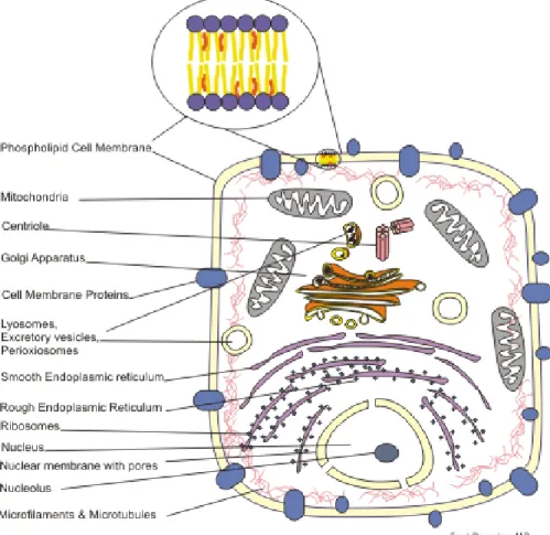
Figure 2.3: Cell structure showing different localizations of proteins.

splice site.

2.3 Protein Localization

One of the goals of analyzing proteins is to determine their function. One indicator of a protein’s function is the cellular localization site of the protein, such as periplasm or the extracellular environment, as shown in Figure2.35_{. Determining the localization of a protein}

through experiments is time consuming and laborious, but can also be determined from the amino acid sequence of the protein, using computational tools.

5_{Image by Boumphreyfr - Own work, CC BY-SA 3.0,}

(26)

Chapter 3 Related Work

The following sections present previous related work. Section 3.1 presents machine learning approaches for splice site prediction, Section 3.2 presents computational tools for protein localization, and the following sections present machine learning methods used when there is a limited amount of labeled data: Section3.3presents semi-supervised classifiers, Section3.4 presents domain adaptation classifiers, and Section3.5presents different ways to incorporate unlabeled data.

3.1 Splice Site Prediction

Most of the approaches addressing splice site prediction involve supervised learning. For example, Li et al. (2012) proposed a method that used the discriminating power of each position in the DNA sequence around the splice site, estimated using the chi-square test. They used a support vector machine algorithm with a radial basis function kernel that combines the scaled component features, the nucleotide frequencies at conserved sites, and the correlative information of two sites, to train a classifier for the human genome. Baten et al. (2006), Sonnenburg et al. (2007), and Zhang et al. (2006), also proposed supervised support vector machine classifiers, whereas Baten et al. (2007) proposed a method using a

(27)

hidden Markov model, Cai et al. (2000) proposed a Bayesian network algorithm, andArita et al. (2002) proposed a method using Bahadur expansion truncated at the second order. For more work on gene prediction using supervised learning, see the survey by Al-Turaiki et al. (2011). However, one major drawback of these supervised algorithms is that they typically require large amounts of labeled data to train a classifier. There are also evidence-based methods, such as TWINSCAN (Korf et al. 2001), CONTRAST (Gross et al. 2007), TrueSight (Li et al. 2013), and using single-molecule transcript sequencing (Minoche et al. 2015). It is however unfair to compare these with ab initio methods, as they use mRNA evidence to generate their models, whereas ab initio methods do not.

3.2 Protein Localization

Numerous computational methods for predicting protein localization are available (for a review see (Emanuelsson 2002)). PSORTb (Gardy et al. 2003) is one of the first widely used method. It uses a Bayesian network to combine the output of several modules – homology analysis, motif-based analysis, detection of transmembrane alpha-helices, outer membrane protein motif analysis, signal peptide predictor, and amino acid composition analysis using SVM – to generate protein localization predictions. Although the classification precision was high, its predictive coverage was low and only applicable to Gram-negative bacteria. An updated version, PSORTb v.2.0 (Gardy et al. 2005), increased the previous version’s coverage and expanded it to include Gram-positive bacteria. It also uses a Bayesian network to combine the output of several modules. The amino acid composition analysis module was updated to use a new SVM-based method, the signal peptide predictor was trained with Gram-positive and Gram-negative data, and the homology and motif modules searched against expanded databases. Another method, TargetP (Emanuelsson et al. 2000), trains a neural network using only the N-terminal sequence information to discriminate between proteins.

(28)

3.3 Semi-supervised Classifiers

An alternative, when the amount of labeled data is not enough for learning a supervised classifier, is to use the limited amount of labeled data in conjunction with abundant unla-beled data to learn a semi-supervised classifier. For example, Nigam et al. (2000) showed empirically that combining a small labeled dataset with a large unlabeled dataset from the same or different domains can reduce the classification error of text documents by up to 30%. Their algorithm uses a combination of Expectation Maximization and the Na¨ıve Bayes classifier by first learning a classifier on the labeled data which is then used to classify the unlabeled data. The combination of these datasets trains a new classifier and iterates un-til convergence. By incorporating unlabeled data, a semi-supervised classifier requires less labeled data than a supervised classifier, to learn an accurate model.

However, semi-supervised classifiers could be misled by the unlabeled data, especially when there is hardly any labeled data (Catal and Diri 2009). For example, if during the first iteration one or more instances are misclassified, the semi-supervised algorithm will be skewed towards the mislabeled instances in subsequent iterations. Another deficiency of semi-supervised classifiers is that their accuracy decreases as the imbalance between classes increases. This is a major challenge for the task of splice site as the classes are highly imbalanced, with only about one percent positive instances. Note that these two chal-lenges affect other algorithms (e.g., domain adaptation), and the data imbalance challenge is common to other problems as well, such as intrusion detection, medical diagnosis, risk management, and text classification, to name a few. The proposed solutions address this problem at the algorithmic level or at the data level through resampling. For an overview of solutions to imbalanced data sets see (Chawla et al. 2004, He and Garcia 2009). For splice site prediction, Stanescu and Caragea(2014a) studied the effects of imbalanced data on semi-supervised algorithms and found that although self-training that adds only positive instances in the semi-supervised iterations achieved the best results out of the methods eval-uated, oversampling and ensemble learning are better options when the positive-to-negative

(29)

ratio is about 1:99. In their subsequent study (Stanescu and Caragea 2014b), they eval-uated several ensemble-based semi-supervised learning approaches, out of which, again, a self-training ensemble with only positive instances produced the best results. However, the highest area under precision-recall curve for the best classifier was 54.78%.

3.4 Domain Adaptation Classifiers

Another option that addresses the lack of abundant labeled data needed with supervised al-gorithms is to use domain adaptation. This approach has been successfully applied to other problems even when the base learning algorithms used in domain adaptation make simplify-ing assumptions. For instance, in text classification, Dai et al.(2007) proposed an iterative algorithm derived from na¨ıve Bayes that uses expectation-maximization for classifying text documents into top categories. This algorithm performed better than supervised SVM and na¨ıve Bayes classifiers when tested on datasets from Newsgroups, SRAA and Reuters. A similar domain adaptation algorithm derived from the Na¨ıve Bayes classifier is the Adapted Na¨ıve Bayes classifier (Tan et al. 2009), which identifies and uses only the generalizable features from the source domain, and the unlabeled data with all the features from the target domain to build a classifier for the target domain. This algorithm was evaluated on the task of sentiment analysis. The prediction rate was promising, with Micro F1 values between 0.69 and 0.90, and Macro F1 values between 0.59 and 0.91. However, the classifier did not use any labeled data from the target domain. For more work on domain adaptation and transfer learning, see the survey by Pan and Yang (2010).

Even though domain adaptation has been used with good results in other domains, there are only a few domain adaptation methods proposed for biological problems. In a recent approach for splice site prediction, Giannoulis et al. (2014) proposed a modified version of the k-means clustering algorithm that took into account the commonalities between the source and target domains for splice site prediction. This algorithm was not very accurate

(30)

though. Its best area under receiver operating characteristic curve (auROC) was below 70%. The best results for the task of splice site prediction, especially when the source and target domains were not closely related, were obtained with a dual-task learning support vector machine classifier proposed by Schweikert et al. (2008), SVMS,T, which used a weighted degree kernel proposed by R¨atsch et al. (2007). Schweikert et al. (2008) used the kernel to generate values between 0 and 1 by normalizing the count of identical dimers at the same position within two DNA fragments of length 141. With this kernel, they solved both classification problems concurrently, for the source and for the target domains, by coupling their solutions via a regularization term. This classifier though did not utilize the abundant unlabeled data from the target domain.

3.5 Usage Styles for Unlabeled Data

If the abundant unlabeled data from the target domain is incorporated one needs to explore the two main methods of using unlabeled data when training a classifier: by assigning hard labels with self-training, or by assigning soft labels with an expectation-maximization (EM) algorithm.

The self-training algorithm (Maeireizo et al. 2004, Riloff et al. 2003, Yarowsky 1995) is an iterative method of using the unlabeled data, that first learns a classifier from only the labeled data. This classifier is then used on the unlabeled data to generate more hard-labeled examples by selecting the instances most confidently classified and assigning labels to them. These instances are then moved from the unlabeled data to the labeled data, and this process is repeated until the classifier converges or a set number of iterations has been reached. This approach has been effective for diverse applications, such as text classification (Blum and Mitchell 1998), optical character recognition (Zhu and Ghahramani 2002), and face recognition (Roli and Marcialis 2006), to name a few.

(31)

itera-tive method for using unlabeled data. In the expectation step, the likelihood is evaluated using the current parameters, whereas in the maximization step the parameters are com-puted by maximizing the expected likelihood evaluated in the expectation step. The label assigned to each instance from the unlabeled data set, that maximizes this expected like-lihood, is a soft label. Similar to the self-training algorithm, this process is repeated until convergence or until reaching the maximum number of iterations.

The EM algorithm was implemented for diverse applications, such as text classification, and biological sequences classification, in domain adaptation settings. For instance, in text classification, the Na¨ıve Bayes Transfer Classification algorithm (Dai et al. 2007), assumes that the source and target data have different distributions. It trains a classifier on source data and then applies the EM algorithm to fit the classifier for the target data, using the Kullback-Liebler divergence to determine the trade-off parameters in the EM algorithm. When tested on datasets from Newsgroups, SRAA and Reuters for the task of top-category classification of text documents this algorithm performed better than support vector machine and Na¨ıve Bayes classifiers.

Another study of EM for text classification (Nigam et al. 2000) used a combination of EM and the Na¨ıve Bayes classifier by first learning a classifier on the labeled data which is then used to classify the unlabeled data. The combination of these datasets trained a new classifier and iterated until convergence. By augmenting the labeled data with unlabeled data the classifier required less labeled data as compared to using only labeled data with a supervised classifier. This algorithm reduced the classification error of text documents by up to 30%.

Both of these methods make one or more of the following assumptions when using the unlabeled data. The self-training algorithm assumes that: instances that are close to each other in the hyperspace have the same label (the smoothness assumption), instances form discrete clusters with instances in a cluster having the same label (the cluster assumption), and instances can be represented in a lower dimensional space than the input space without

(32)

significant loss of information (the manifold assumption). The expectation-maximization algorithm makes the assumption that there are features with missing values or that a simpler model can be learned by using additional unobserved instances.

Therefore, when it cannot be determined a priori if these assumptions are valid for the data set used, one should evaluate both methods, and the combination of both, to determine which one works best for the data set and the algorithm used.

(33)

Chapter 4 Supervised Classifiers

Several domain adaptation methods were proposed, derived from the na¨ıve Bayes, and the regularized logistic regression supervised classifiers. Before describing the proposed methods the supervised classifiers are presented, as these are used as baselines, and to highlight the differences between the proposed methods and these classifiers.

4.1 Multinomial Na¨ıve Bayes

The multinomial na¨ıve Bayes classifier (McCallum et al. 1998) assumes that the sample data used to train the classifier is representative of the population data on which the clas-sifier will be used. In addition, it assumes that the frequency of the words determines the label assigned to an instance, and that the position of a word is irrelevant (the na¨ıve Bayes assumption). Thus, using Bayes’ property a classifier can approximate the posterior proba-bility, i.e., the probability of a class given an unclassified instance, as being proportional to the product of the prior probability of the class, and the probability of the instance given the class:

(34)

where the probability of the class is P(yi =y) = m X i=1 1(yi =y) m (4.2)

with ₁(yi =y) = 1 if yi =y, and 0 otherwise.

The probability of an instance given its class is the multinomial distribution:

P(xi |yi =y) = P(|xi|)|xi|! n Y j=1 P(xj |yi =y)x i j xi j! (4.3) where P(xj |yi =y) = 1 + m X i=1 xi_j₁(yi =y) n+ n X k=1 m X i=1 xi_k₁(yi =y) and P(|xi|) = P(|xi|=l) = m X i=1 1(|xi|=l) m

The document length is included in Equation (4.4) because it specifies the number of draws from the multinomial, with the assumption that the document length is not dependent on class.

4.2 Na¨ıve Bayes

Similar to the multinomial na¨ıve Bayes classifier, the multivariate Bernoulli na¨ıve Bayes classifier assumes that the position of a feature is irrelevant (the na¨ıve Bayes assumption), though, unlike the multinomial na¨ıve Bayes classifier, it represents each instance as a vector of binary features indicating whether the corresponding feature occurs in the instance or not. It also uses Bayes’ property to approximate the posterior probability, using Equation (4.1).

(35)

The probability of an instance given its class is the product of probabilities of all feature values, including the probability of non-occurrence for features that do not occur in the instance: P(xi |yi =y) = n Y j=1 xi_jP(xj |yi =y) + (1−xij) 1−P(xj |yi =y) (4.4) where P(xj |yi =y) = 1 + m X i=1 xi_j₁(yi =y) 2 + m X i=1 1(yi =y)

4.3 Regularized Logistic Regression

Given a set of training instances generated independentlyX ∈_Rm×n_{and their corresponding}

labels Y ∈ Ym_, _Y ₌ _{₀_,₁_}_{, with} _m _{the number of training instances and} _n _{the number of}

features, logistic regression models the posterior as (Le Cessie and Van Houwelingen 1992):

P(yi =y|xi;θ) =      g(θTxi) ,if y= 1 1−g(θTxi) ,if y= 0 =g(θTxi)y · 1−g(θTxi)1−y

where g(·) is the logistic function g(θT_xi_{) =} 1 1+e−θT xi.

With this model, the log likelihood can be written as a function of the parameters θ as follows: l(θ) = log m Y i=1 P(y|xi;θ) = log m Y i=1 g(θTxi)y · 1−g(θTxi)1−y = m X ylogg(θTxi) + (1−y) log 1−g(θTxi)

(36)

The parameters are estimated by maximizing the log likelihood, usually using maximum entropy models, after a regularization term, with parameter λ, is introduced to penalize large values of θ: θ= arg max θ l(θ)−λkθk2 (4.5)

Note that xi _{is the}_ith _{sequence in the training data set,}_yi _{is the corresponding label of}

xi_{, and} _xi

(37)

Chapter 5 Domain Adaptation Classifiers

One limitation of the supervised classifiers is that when trained on one domain and then used on a different domain, in most cases, their classification accuracy decreases. The first method proposed to address this issue, used the Adapted Na¨ıve Bayes classifier proposed by Tan et al.(2009), with two modifications: the labeled data from the target domain was used, and the self-training technique to assign labels to instances from target unlabeled dataset was employed. These modifications will be described in more detail shortly. The second method proposed further modified this algorithm: normalized the counts used in computing the prior and the likelihood, used mutual information instead of probabilities when ranking the source domain features, and used different representation for the input data. The third method proposed is derived from a discriminative classifier instead of generative one, namely, regularized logistic regression. The last method proposed assigned different weights to the labeled data from the source and target domains, then trained a supervised classifier on the combined dataset.

(38)

5.1 Semi-supervised Domain Adaptation Classifier

De-rived from Multinomial Na¨ıve Bayes with Counts

of

k

-mer Features

The first step of this classifier is to identify in the source domain the subset of the features that generalize well and are highly correlated with the label. Then, use the data from the source domain with only these features and the data from the target domain with all the features to predict the labels of the test instances in the target domain. Theoretically, the set of features in each domain can be split into four categories, based on two selection criteria. Based on the correlation between the feature and the label, the features can be divided into features that are highly related to the labels, and features that are less related to the labels. Based on the specificity of the features, the features can be divided into features that are very specific to a domain, and features that generalize well across related domains, as shown in Figure 5.1.

To select informative features from the source domain the features are ranked based on their probabilities. The features that are generalizable between source and target domains would most likely occur frequently in both domains, and should be ranked higher. In addi-tion, the features that are correlated to the labels should also be ranked higher. Therefore,

Figure 5.1: The features of interest are generalizable and highly correlated to class, i.e., the ones in the highlighted quadrant.

(39)

the following measure is used to rank the features in the source domain:

f(xj) = log

PtSL(xj)·PtT L(xj)

|PtSL(xj)−PtT L(xj)|+α

(5.1)

where PtSL andPtT L are the probability of the feature xj,∀j ∈ {1, . . . , n}in the source and

target domain, respectively. The numerator ranks higher the features that occur frequently in both domains, since the larger both probabilities are the larger the numerator is, and thus the higher the rank of the feature is. The denominator ranks higher the features that have similar probabilities (i.e., the generalizable features), since the closer the probabilities are for a feature in both domains, the smaller the denominator value is, and thus the higher the rank. The additional value in the denominator, α, is used to prevent division by zero. The higher its value is the more influence the numerator has in ranking the features, and vice versa. To limit its influence on ranking the features, a small value was chosen for this parameter, 0.0001. The probability of a feature in either domain is

P(xj) = m X i=1 xi_j+β m X i=1 n X j=1 xi_j +m·β (5.2)

where β is a smoothing factor, which is used to prevent the probability of a feature to be 0 (which would make the numerator in Equation (5.1) equal to 0, and the logarithm function is undefined for 0). A small value was chosen for β as well, 0.0001, to limit its influence on the ranking of features. Note that the values for α and β do not have to be the same, but they can be, as used by Tan et al.(2009) and in these experiments.

Once the domain specific features of the source domain are filtered out, the algorithm uses a combination of the expectation-maximization (EM) algorithm and a weighted multinomial na¨ıve Bayes algorithm. Similar to theEM algorithm, it has two steps that are iterated until convergence. The first step, the M-step, simultaneously estimates the class probability

(40)

and the class conditional probability of a feature. However, unlike the EM algorithm that uses the data from one domain to calculate these values, this algorithm uses a weighted combination of the data from the source domain and the target domain.

P(yi =y) = (1−λ) mtSL X i=1 1(yi =y) +λ mtT L X i=1 1(yi =y) (1−λ)mtSL+λmtT L (5.3) P(xj |yi =y) = (1−λ) mtSL X i=1 ηjxij1(y i ₌_y_{) +}_λ mtT L X i=1 xi_j₁(yi =y) + 1 (1−λ) n X k=1 mtSL X i=1 ηkxik1(y i ₌_y_{) +}_λ n X k=1 mtT L X i=1 xi_k₁(yi =y) +n (5.4)

where λ is the weight factor between the source and target domains:

λ= min{δ·τ,1} (5.5)

and τ is the iteration number. δ∈(0,1) is a constant that determines how fast the weight shifts from the source domain to the target domain, and ηj is 1 if feature xj in the source

domain is a generalizable feature, 0 otherwise.

Unlike the algorithm proposed byTan et al.(2009), which considers that all the instances from the target domain are unlabeled and does not use them during the first iteration (i.e., λ = 0), it is reasonable to assume that there is a small number of labeled instances in the target domain, and the proposed algorithm uses any labeled data from the target domain in the first and subsequent iterations. In the first iteration only labeled instances from the source and target domains are used to estimate the probability distributions for the class conditional probabilities given the instance. In subsequent iterations the class of the instance for the labeled data from the source and target domains and the probability distribution of the class for the unlabeled data from the target domain are used.

(41)

the values obtained from the M-step. P(yi =y|xi)∝P(yi =y)P(|xi|)|xi|! n Y j=1 P(xj |yi =y)x i j xi j! (5.6)

The second modification made to the classifier proposed by Tan et al.(2009), is the use of self-training, i.e., at each iteration, the instances with the top class probability are se-lected, proportional to the class distribution, and considered to be labeled in the subsequent iterations. This improves the prediction accuracy of the classifier because it does not allow the unlabeled data to alter the class distribution from the target labeled data.

The two steps, E andM, are repeated until the instance conditional probabilities values in Equation (5.6) converge (or a given number of iterations is reached). The algorithm is summarized in Algorithm 1, and shown in Figure 5.2.

Algorithm 1 Outline of the semi-supervised domain adaptation classifier derived from multinomial na¨ıve Bayes, SSh+sDAk_MNB-mers.

1: Select generalizable features from the source domain, i.e., the top ranked features using Equation (5.1).

2: For each class simultaneously estimate the class probability and the class conditional probability of each feature using Equations (5.3) and (5.4), respectively. For the source domain use all labeled instances, and only the generalizable features. For the target domain use only labeled instances, and all features.

3: Self-training: Select, proportional to the prior class distribution, the target instances with the top class probability, and consider these to be labeled (i.e., assign them hard-labels) in the subsequent iterations; assign soft-labels to the remaining instances. 4: while labels assigned to unlabeled data change do

5: M-step: Same as step 2 but use the class for labeled and self-trained instances from the target domain, and the class distribution for unlabeled instances.

6: Same as step 3.

7: E-step: Estimate the class distribution for unlabeled training instances from the target domain using Equation (5.6).

8: end while

(42)

Figure 5.2: Semi-supervised domain adaptation classifier derived from multinomial na¨ıve Bayes.

5.1.1 Data Sets

Three data sets from two biological problems – protein localization, and splice site prediction – were used to evaluate this and the other proposed methods.

Protein Localization

For protein localization the following two datasets were used:

• The PSORTb v2.01 _{dataset (Gardy et al. 2005), first introduced in (Gardy et al. 2003).}

It contains proteins from two related prokaryotes, gram-negative and gram-positive bacteria, and their primary localization: cytoplasm, inner membrane, periplasm, outer membrane, and extracellular space. Only instances with classes that appear in both datasets were used: 480 proteins from gram-positive bacteria (194 from cytoplasm, 103 from inner membrane, and 183 from extracellular space) and 777 proteins from 1_{Downloaded from}

(43)

(a) Prokaryotes (b) Eukaryotes

Figure 5.3: Number of proteins used from each dataset. From the PSORTb v2.0 dataset 194 proteins localized in cytoplasm, 103 in inner membrane, and 183 in extracellular space, were used for gram-positive, and 278 proteins localized in cytoplasm, 309 in inner mem-brane, and 190 in extracellular space, for gram-negative. From the TargetP dataset 368 mitochondrial, 269 secretory pathway, and 162 “other” proteins from plant were used, and 371 mitochondrial, 715 secretory pathway, and 1,652 “other” proteins from non-plant.

gram-negative bacteria (278 from cytoplasm, 309 from inner membrane, and 190 from extracellular space), as shown in Figure 5.3a.

• The TargetP2 dataset, first introduced in (Emanuelsson et al. 2000). It contains proteins from two distantly related organisms, plant and non-plant, and their primary sub-cellular localization: mitochondrial, chloroplast, secretory pathway, and “other.” Similar to the bacteria proteins, from this data set 799 plant proteins were used (368 mitochondrial, 269 secretory pathway and 162 “other”) and 2,738 non-plant proteins (371 mitochondrial, 715 secretory pathway and 1652 “other”), as shown in Figure5.3b.

Splice Site

For splice site prediction the dataset3 _{first used in (Schweikert et al. 2008) was used, which}

contains sets of 141 nucleotides-long DNA sequences from five organisms. Each sequence has 2_{Downloaded from}

http://www.cbs.dtu.dk/services/TargetP/datasets/datasets.php 3_{Downloaded from}

(44)

Figure 5.4: DNA fragments of 141 bp and their labels indicating whether the AG dimer at index 61 is a splice site or not.

the AG dimer at sixty-first position and a label associated with the sequence that indicates whether this dimer is an acceptor splice site or not, as shown in Figure 5.4. The five organ-isms areC.elegansas source organism, and four target organisms at increasing evolutionary distance from C.elegans: C.remanei, P.pacificus, D.melanogaster, and A.thaliana. For the source organism there is one fold of 100,000 instances, whereas for the target organisms there are three folds with 1,000, 2,500, 6,500, 16,000, 25,000, 40,000, and 100,000 instances that can be used for training, and three corresponding folds of 20,000 instances that can be used for testing. For the target organisms the datasets with 2,500, 6,500, 16,000, 40,000, and 100,000 instances were used, as shown in Figure5.5. In each file there are about 1% positive instances (i.e., DNA sequences in which the AG dimer at sixty-first position is an acceptor splice site) and the remaining instances are negative. Note that although the dataset used has only acceptor splice sites, the problem of predicting donor splice sites can be addressed with the same approach.

5.1.2 Experimental Setup

Two types of features were used to represent the data. In one representation, a sliding window approach was used to count the k-mer frequencies, and represent each sequence as the count ofk-mer occurrences. This representation was used with this domain adaptation classifier for both problems: protein localization, and splice site prediction. The other type of features – in which each sequence was converted into a set of features that represent the

(45)

Figure 5.5: For the source organism,C.elegans, there is one fold of 100,000 instances, whereas for the target organisms – C.remanei, P.pacificus, D.melanogaster, and A.thaliana – there are three folds with 2,500, 6,500, 16,000, 40,000, and 100,000 instances that can be used for training, and three corresponding folds of 20,000 instances that can be used for testing. In each file there are about 1% positive instances and about 99% negative instances.

nucleotides present in the sequence at each position, and the 3-mer at each position – was used only with the other domain adaptation proposed, and for the splice site prediction.

Each amino-acid sequence was represented as a count of occurrences of k-mers. A sliding window approach was used to count thek-mer frequencies. For example, a cytoplasm protein starting withLLRSYRS. . .would be represented in WEKA ARFF format, when using 2-mers, as: @RELATION rel @ATTRIBUTE 2-MER AA . . . @ATTRIBUTE 2-MER VV

(46)

@DATA

1,. . .,1,. . .,2,. . .,1,. . .,1,. . .,cytoplasm

which are the counts corresponding to the occurrences of features LL, LR, RS, SY, and YR, respectively.

Splice Site Prediction

Three representations for nucleotide sequences were used. In one representation, a sliding window approach was used to count the 8-mer frequencies, and represent each sequence as the count of 8-mer occurrences (the other two representations are described in Section 5.2). For example, a DNA sequence starting with AAGATTCGC... and label -1 would be repre-sented in WEKA ARFF format as:

@RELATION rel

@ATTRIBUTE 8-MER AAAAAAAA .

. .

@ATTRIBUTE 8-MER AAGATTCG .

. .

@ATTRIBUTE 8-MER AGATTCGC . . . @ATTRIBUTE 8-MER TTTTTTTT @ATTRIBUTE cls {1,-1} @DATA 1,. . .,1,. . .,-1

which are the counts corresponding to the occurrences of 8-mers AAGATTCG and AGATTCGC, respectively. This representation was used with only this semi-supervised domain adaptation classifier.

(47)

Data Splits and Metrics Used Protein Localization

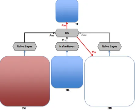
In order to obtain unbiased estimates for classifier performance five-fold cross validation was used. All labeled data from the source domain for training (tSL) was used and the target domain data was randomly split into 3 sets: up to 20% used as labeled data for training (tTL), up to 60% used as unlabeled data for training (tTU), and 20% used as test data (TT), and the classifier was trained on tSL + tTL + tTU and tested on TT, as shown in Figure 5.6.

To evaluate the classifier with these data, the area under the receiver operating charac-teristic (auROC) was used, as the class distributions are relatively balanced.

For the splice site prediction there are 3 folds for each target organism. To limit the number of experiments, the following datasets were used:

• The 100,000 C.elegans instances as source labeled data used for training (tSL).

• Only the sets with 2,500, 6,500, 16,000, and 40,000 instances as labeled target data used for training (tTL).

Figure 5.6: Experimental setup for protein localization: 3 datasets are used to train the classifier – source domain labeled (tSL), target domain labeled (tTL), and target domain unlabeled (tTU) – and 1 to test it – target domain labeled (TT).

(48)

(a) First fold: auROC = 0.9331 (b) First fold: auPRC = 0.2132

Figure 5.7: auROC and auPRC values for supervised domain adaptation classifier derived from the regularized logistic regression, described in Section5.3.2. This classifier was trained with one of the three folds of target labeled data from A.thaliana with 2,500 instances. The auROC is 0.9331, suggesting a highly accurate classifier. A more accurate picture, in terms of classifier’s performance for imbalanced datasets, is given by auPRC. Its corresponding value is 0.2132.

• The set with 100,000 instances as unlabeled target data used for training (tTU), and also as validation dataset.

• The corresponding folds of the 20,000 instances as target data used for testing (TT). Then the results are averaged over the 3 folds to obtain unbiased estimates. For semi-supervised algorithms, the classifier was trained on tSL + tTL + tTU and tested on TT, whereas for supervised algorithms, the classifier was trained on tSL + tTL and tested on TT.

To evaluate the classifiers with these data, the area under precision-recall curve (auPRC) was used, a metric that is preferred over area under a receiver operating characteristic curve when the class distribution is skewed (Davis and Goadrich 2006), as shown in Figure 5.7.

Research Questions

This experimental setup was used to answer several general questions (Q1, Q2, and Q3), and several classifier specific questions (Q4, Q5, and Q6). Specifically, how does the performance of the classifier vary with:

(49)

Q2 Variation with the amount of target labeled/unlabeled data?

Q3 The distance between the source and target domains?

Q4 Number of features used in the target domain (i.e., keep all features, remove at most 50% of the least occurring features)?

Q5 Number of features retained in the source domain after selecting the generalizable features?

Q6 The choice of the source and target domains (for protein localization)?

As baselines, this classifier was compared with the multinomial na¨ıve Bayes classifier trained on all source data, NBtSL, the multinomial na¨ıve Bayes classifier trained on 5% target

data, NBtT L(5%), and the multinomial na¨ıve Bayes classifier trained on 80% target data, NBtT L(80%). Each classifier was tested on 20% of target data. The expectation is that the prediction accuracy of this classifier will be lower bounded by NBtT L(5%), upper bounded by NBtT L(80%), and better than NBtSL.

As baseline, this classifier was compared with the best overall algorithm in Schweikert et al. (2008).

5.1.3 Results and Discussion

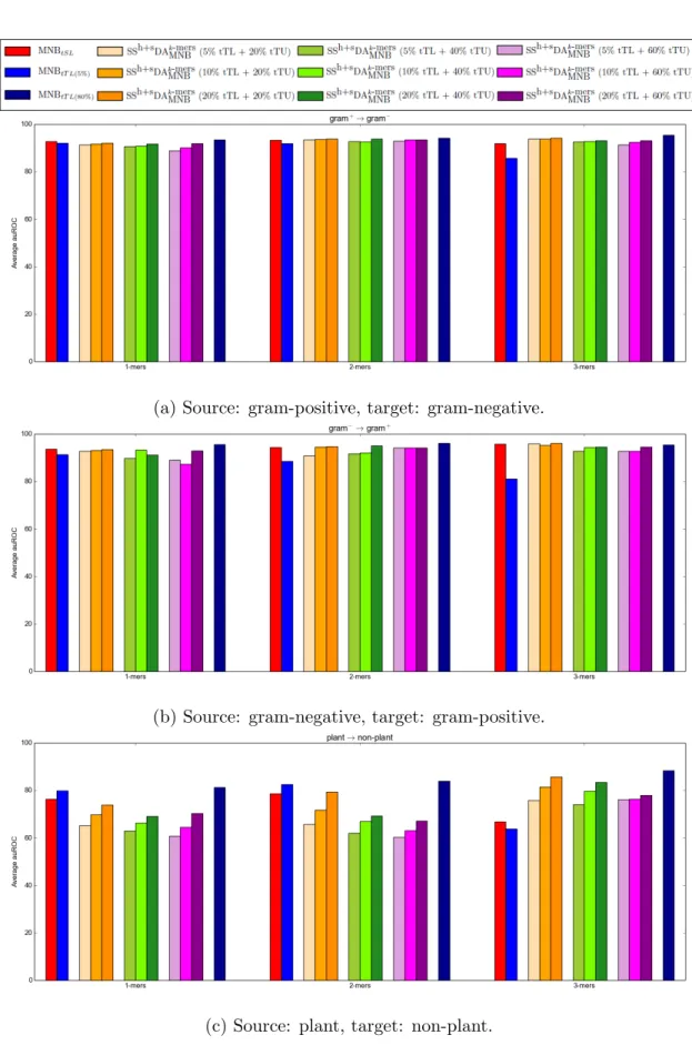
Table 5.1 and Figure 5.8 show the average auROC values over the five-fold cross validation trials for this algorithm and for the baseline algorithms. From these results the following

(50)

(a) Source: gram-positive, target: gram-negative.

(b) Source: gram-negative, target: gram-positive.

(c) Source: plant, target: non-plant.

Figure 5.8: Results of the semi-supervised domain adaptation classifier derived from multi-nomial na¨ıve Bayes with counts of k-mer features on protein data.

(51)

Table 5.1: A comparison, on the protein localization task, between the domain adaptation classifier, SSh+sDAk_MNB-mers, the multinomial na¨ıve Bayes classifier trained on all source data, MNBtSL, the multinomial na¨ıve Bayes classifier trained on 5% target data MNBtT L(5%), and the multinomial na¨ıve Bayes classifier trained on 80% target data, MNBtT L(80%). The results

are reported as average auROC values over five-fold cross validation trials. The best values for the domain adaptation classifier are highlighted. Note that SSh+sDAk_MNB-mers is bounded by MNBtT L(5%) and MNBtT L(80%), and that SSh+sDAkMNB-mers predicts more accurately as the length of k-mers increases.

(a) PSORTb dataset: source domain is gram+ and target domain is gram−

Features Classifier Unlabeled Labeled

5% 10% 20% count of 1-mers MNBtSL 92.74 MNBtT L(5%) 92.18 SSh+sDAk_MNB-mers 20% 91.42 91.70 92.08 40% 90.68 90.82 91.68 60% 89.00 90.20 91.90 MNBtT L(80%) 93.52 count of 2-mers MNBtSL 93.30 MNBtT L(5%) 91.90 SSh+sDAk_MNB-mers 20% 93.58 93.66 93.94 40% 92.84 92.68 93.90 60% 92.92 93.58 93.50 MNBtT L(80%) 94.24 count of 3-mers MNBtSL 91.94 MNBtT L(5%) 85.80 SSh+sDAk_MNB-mers 20% 93.80 93.80 94.24 40% 92.62 92.78 93.14 60% 91.34 92.40 93.08 MNBtT L(80%) 95.52

A1 In terms of features used, the best results were obtained when using 3-mers as features – an example is shown in Figure 5.9. This makes sense since longer k-mers capture more information associated with the relative position of each amino-acid. When using 3-mers, the proposed algorithm provides between 9.84% and 34.14% better clas-sification accuracy when compared to multinomial na¨ıve Bayes classifier trained on 5% of the labeled data from the target domain, and between 0.37% and 28.2% when compared to the multinomial na¨ıve Bayes classifier trained on labeled data from the

(52)

Table 5.1: (Cont.)

(b) PSORTb dataset: source domain is gram− and target domain is gram+

source domain, except when the plant proteins are the target domain.

A2 For most cases, the largest auROC values for this algorithm were obtained when using the least amount of target unlabeled data – an example is shown in Figure 5.10a. This would suggest that even though using unlabeled data is beneficial, using too much unlabeled data is detrimental because the unlabeled instances may act as noise and corrupt the prediction from the target labeled data. In addition, intuitively, using more labeled data from the target domain should lead to better prediction accuracy. This was indeed the case with this classifier – as shown in the example in Figure5.10b.

A3 When the source and target domains are close the classifier learned is better. For example, the auROC is higher for the PSORTb datasets than for the TargetP datasets.

(53)

(d) Source: non-plant, target: plant.

Figure 5.8: (Cont.)

Figure 5.9: Comparison between results obtained when using 1-mers, 2-mers, and 3-mers as features with the semi-supervised domain adaptation classifier derived from multinomial na¨ıve Bayes. Best results were obtained using 3-mers.

(54)

(a) Best results were obtained when using the least amount of target unlabeled data.

(b) Best results were obtained when using the most amount of target labeled data.

Figure 5.10: Comparison between results obtained when using different amounts of target labeled, and target unlabeled data with the semi-supervised domain adaptation classifier derived from multinomial na¨ıve Bayes.

(55)

Table 5.1: (Cont.)

(c) TargetP dataset: source domain is plant and target domain is non-plant

Therefore, the closer the target domain is to the source domain the better the classifier learned.

A4 When trying to establish how many features from the target domain should be used it was determined that removing any features does not improve the performance of the proposed algorithm.

A5 When trying to ascertain how many features from the source domain should be kept after ranking them with Equation (5.1), it was determined that the best results were obtained when at least 50% of the features were kept, i.e., the 50% top-ranked features and any other features with the same rank as the last feature kept.

(56)

Table 5.1: (Cont.)

(d) TargetP dataset: source domain is non-plant and target domain is plant

when the negative proteins were used as the source domain than when the gram-positive proteins were used as the source domain. Similarly, for the TargetP dataset, better predictions were obtained when using non-plant proteins as the source domain than when using plant proteins as the source domain. This is because in both cases there were more gram-negative instances and more non-plant instances, respectively, than gram-positive instances and plant instances, respectively.

It is interesting to note that in some instances the multinomial na¨ıve Bayes classifier trained on the source domain performed better than this algorithm. This occurred mainly when this algorithm used 5% or 10% of the target labeled data and when the features were 1-mers or 2-mers. However, this is somewhat expected, as using very little labeled data from the target domain does not provide a representative sample for the population, and using short

(57)

k-mers does not capture the relative position of the amino-acids.

Although this algorithm worked well for the protein localization task, it performed poorly on the splice site prediction task, as shown in Table 5.2. This algorithm always gravitated towards classifying each instance as not containing a splice site. This is due mainly because the 8-mers indicating a splice site occur with low frequency and their relative position to the splice site is important.

From these results the following observations can be made:

A2 The auPRC values for this algorithm were very similar regardless of the amount of target labeled data.

A3 The classification performance of this algorithm did not decrease as the distance be-tween the source and target domains increased, as one would have expected.

A4 Similar to protein localization task, removing any features does not improve the per-formance of this algorithm.

A5 In terms of the number of features from the source domain to keep after ranking them with Equation (5.1), it was determined that the best results were obtained when at least 50% of the features were kept, i.e., the 50% top-ranked features and any other features with the same rank as the last feature kept.

The last two observations suggest that the features need to take into consideration the locations of the 8-mers to improve the classification accuracy of this classifier on the splice site prediction task.

(58)

Table 5.2: auPRC values for the 4 target organisms based on the number of labeled target instances used for training: 2,500, 6,500, 16,000, and 40,000. For comparison with this algo-rithm the values for the best overall supervised domain adaptation algoalgo-rithm inSchweikert et al. (2008), SVMS,T, are shown as S DASVM.

(a)C.remanei 2,500 6,500 16,000 40,000 SSh+sDAk_MNB-mers 1.13 1.13 1.13 1.10 S DASVM 77.06 77.80 77.89 79.02 (b) P.pacificus 2,500 6,500 16,000 40,000 SSh+sDAk_MNB-mers 1.00 0.97 1.07 1.10 S DASVM 64.72 66.39 68.44 71.00 (c) D.melanogaster 2,500 6,500 16,000 40,000 SSh+sDAk_MNB-mers 1.07 1.13 1.07 1.03 S DASVM 40.80 37.87 52.33 58.17 (d)A.thaliana 2,500 6,500 16,000 40,000 SSh+sDAk_MNB-mers 1.20 1.17 1.20 1.17 S DASVM 24.21 27.30 38.49 49.75

5.2 Semi-supervised Domain Adaptation Classifiers

De-rived from Na¨ıve Bayes with Location-Aware

Fea-tures for the task of Splice Site Prediction

One major drawback of the previous algorithm is that during the first iterations it assigns low weight to the target data, including the labeled data, through λ in (Equations (5.3) and (5.4)). This biases the classifier towards the source domain. However, it is not effective to only assign a different weight to the target labeled data in Equations (5.3) and (5.4). This is because when there are much more labeled instances from the source domain, as well as much more unlabeled instances from the target domain, i.e., mtSL mtT L and

Domain adaptation algorithms for biological sequence classification

DOMAIN ADAPTATION ALGORITHMS FOR BIOLOGICAL

SEQUENCE CLASSIFICATION

by

NIC HERNDON

B.S., University of Nevada, Reno, 2004

M.S., University of Nevada, Reno, 2008

AN ABSTRACT OF A DISSERTATION

submitted in partial fulfillment of the

requirements for the degree

DOCTOR OF PHILOSOPHY

Department of Computer Science

College of Engineering

KANSAS STATE UNIVERSITY

Manhattan, Kansas

Abstract

DOMAIN ADAPTATION ALGORITHMS FOR BIOLOGICAL

SEQUENCE CLASSIFICATION

by

NIC HERNDON

B.S., University of Nevada, Reno, 2004

M.S., University of Nevada, Reno, 2008

A DISSERTATION

submitted in partial fulfillment of the

requirements for the degree

DOCTOR OF PHILOSOPHY

Department of Computer Science

College of Engineering

KANSAS STATE UNIVERSITY

Manhattan, Kansas

2016

Copyright

Nic Herndon

Abstract

Table of Contents

List of Figures

List of Tables

Acknowledgments

Chapter 1

Introduction

Published Contributions Included in this Work

Chapter 2

Background

2.1

Brief Introduction to Machine Learning

2.1.1

Notation

2.1.2

Supervised Classification

2.1.3

Semi-supervised Classification

2.1.4

Supervised Domain Adaptation Classification

2.1.5

Semi-supervised Domain Adaptation Classification

2.2

Central Dogma of Molecular Biology

2.3

Protein Localization

Chapter 3

Related Work

3.1

Splice Site Prediction

3.2

Protein Localization

3.3

Semi-supervised Classifiers

3.4

Domain Adaptation Classifiers

3.5

Usage Styles for Unlabeled Data

Chapter 4

Supervised Classifiers

4.1

Multinomial Na¨ıve Bayes

4.2

Na¨ıve Bayes

4.3

Regularized Logistic Regression

Chapter 5