Using deep Convolutional Neural Network architectures for object classification and detection within X-ray baggage security imagery.

On Using Deep Convolutional Neural Network

Architectures for Object Classification and

Detection within X-ray Baggage Security Imagery

Samet Akcay

*

_{, Mikolaj E. Kundegorski, Chris G. Willcocks, and Toby P. Breckon}

Abstract—We consider the use of deep Convolutional Neural Networks (CNN) with transfer learning for the image classifica-tion and detecclassifica-tion problems posed within the context of X-ray baggage security imagery. The use of the CNN approach requires large amounts of data to facilitate a complex end-to-end feature extraction and classification process. Within the context of X-ray security screening, limited availability of object of interest data examples can thus pose a problem. To overcome this issue, we employ a transfer learning paradigm such that a pre-trained CNN, primarily trained for generalized image classification tasks where sufficient training data exists, can be optimized explicitly as a later secondary process towards this application domain. To provide a consistent feature-space comparison between this approach and traditional feature space representations, we also train Support Vector Machine (SVM) classifier on CNN fea-tures. We empirically show that fine-tuned CNN features yield superior performance to conventional hand-crafted features on object classification tasks within this context. Overall we achieve 0.994 accuracy based on AlexNet features trained with Support Vector Machine (SVM) classifier. In addition to classification, we also explore the applicability of multiple CNN driven detection paradigms such as sliding window based CNN (SW-CNN), Faster RCNN (F-RCNN), Region-based Fully Convolutional Networks (R-FCN) and YOLOv2. We train numerous networks tackling both single and multiple detections over SW-CNN/F-RCNN/R-FCN/YOLOv2 variants. YOLOv2, Faster-RCNN, and R-FCN provide superior results to the more traditional SW-CNN ap-proaches. With the use of YOLOv2, using input images of size 544×544, we achieve 0.885 mean average precision (mAP) for a six-class object detection problem. The same approach with an input of size 416×416 yields 0.974 mAP for the two-class firearm detection problem and requires approximately 100ms per image. Overall we illustrate the comparative performance of these techniques and show that object localization strategies cope well with cluttered X-ray security imagery where classification techniques fail.

Index Terms—Deep convolutional neural networks, transfer learning, image classification, detection, X-ray baggage security

I. INTRODUCTION

X

RAY baggage security screening is widely used to main-tain aviation and transport security and poses a significant image-based screening task for human operators reviewing compact, cluttered and highly varying baggage contents within limited time-scales. The increased passenger throughput, in the global travel network, and the increased focus on broader aspects of extended border security (e.g., freight, shipping, S.Akcay*_{, C.G.Willcocks, T.P.Breckon are with Department of Computer} Science, Durham University, Durham, UK (e-mail: { samet.akcay, christo-pher.g.willcocks, toby.breckon }@durham.ac.uk).

M.E.Kundegorski was with Department of Computer Science, Durham University, Durham, UK.

Asterisk indicates corresponding author.

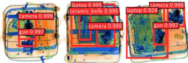
postal) results in a challenging and timely automated image classification task. camera 0.998 laptop 0.995 ceramic_knife 0.996 camera 0.999 gun 0.997 camera 0.998 laptop 0.924 gun 0.997

Fig. 1: Exemplar X-ray baggage imagery multiple objects.

Previous work within this context is primarily based on the bag of visual words model (BoVW) [1]–[5] although there is some limited research using other techniques such as sparse representations [6]. Convolutional neural networks (CNN), a state-of-the-art paradigm for contemporary computer vision problems, were introduced into the field of X-ray baggage imagery by [7], comparing CNN to a BoVW approach with conventional hand-crafted features trained with a Support Vector Machine (SVM) classifier. Following the work of [7], [8] also studies X-ray baggage object classification with CNN similarly comparing it against traditional classifiers.

Motivated by [4], [7], [8], we conduct an extensive set of experiments to evaluate the strength of CNN features and tra-ditional hand-crafted features (SIFT, SURF, FAST, KAZE [4]). As with [7], we perform layer freezing by fixing parameters from the source domain without any further optimization to observe how fixing the layer parameters at varying points in the network influences the overall performance of the transfer learning based tuning of the end-to-end CNN. Furthermore, in contrast to [7], [8] comparing end-to-end CNN classifica-tion with tradiclassifica-tional feature-driven pipelines, we addiclassifica-tionally present results whereby we extract the output of the last layer of a given CNN (f c7 of AlexNet [9]) as a feature map itself.

We subsequently train an SVM classifier, generally used as the final classification stage of feature-driven approaches [1]– [5], to provide a consistent feature-space comparison between both learned (CNN) and traditional feature representations.

In addition to the proposed classification scheme, we ex-plore object detection within this problem domain by inves-tigating both the use of a sliding window paradigm (akin to [5], [10]) and evaluate contemporary approaches to learn efficient object localization via R-CNN [11], R-FCN [12] and YOLOv2 [13] approaches. As shown in previous work [7], [8] the challenging and cluttered nature of object detection in X-ray security imagery often poses additional challenges

for established contemporary classification and detection ap-proaches, such as RCNN/R-FCN [11], [12].

The main contributions of this paper are: (a) the exhaus-tive evaluation of classification architectures of [9], [14]– [16] against prior work in the field from [1], [2], [4], [6], [17], (b) the feature-space comparison of the end-to-end CNN classification results of [7], [8] against the final stage SVM classification on the extracted CNN features, (c) the compari-son of the region based object detection/localization strategies of [11], [12] against the prior strategies proposed in [10], [18]. Contrasting performance results are obtained against the prior published studies of [4], [7] over a comprehensive dataset of 11,627 examples making this the largest combined X-ray object detection and classification study in the literature to date. Moreover, the evaluation is strengthened further by using UK government evaluation dataset [19] (available upon request from UK Home Office Centre for Applied Science and Technology (CAST)). Overall, we identify classification approaches and detection strategies that outperform the prior work of [5], [7], [10].

II. RELATEDWORK

Aviation security screening systems are of interest and have been studied for decades [20]. Computer Aided Screening (CAS) performs automated threat detection in the generalized sense, however this largely remains an unsolved problem. Previous work [21], [22] has focused on image enhancement [23]–[25], segmentation [26], [27], classification [1], [2], [4], [6], [17] or detection [5], [10], [28], [29] tasks in order to further investigate the real time applicability of CAS to automatize aviation security screening. For a detailed overview the reader is directed to Rodgerset al.[22] and Moutonet al.

[21]. Our focus is based on addressing the object classification and detection tasks presented in the following sections.

Classification: For the classification of X-ray objects, the

majority of prior work proposes traditional machine learning approaches based on a Bag-of-Visual-Words (BoVW) feature representation scheme, using hand-crafted features together with a classifier such as a Support Vector Machine (SVM) [1], [2], [4], [6], [17].

The work of [1] considers the concept of BoVW within X-ray baggage imagery using SVM classification with sev-eral feature representations (DoG, DoG+SIFT, DoG+Harris) achieving a performance of0.7recall,0.29precision, and0.57 average precision. Turcsany et al. [2] followed a similar ap-proach and extended the work presented in [1]. Using a BoVW with SURF descriptors and an SVM classifier, together with a modified version of codebook generation, yields 0.99 true positive and 0.04 false positive rates [2]. BoVW approaches with feature descriptor and SVM classification are also used in [3] for the classification of single and dual-view X-ray images, with optimal average precisions achieved for firearms (0.95) and laptops (0.98). Mery et al. [17] propose a recognition approach that applies detection to single-view images to find objects of interest, and then matches these across multiple view X-ray images yielding 0.96precision and0.93recall for 120 objects. A BoVW approach is further employed in [6] where

a dictionary is formed for each class that consists of feature descriptors of randomly cropped image patches. Performance of the model is evaluated by fitting a sparse representation classification to the extracted feature descriptors of randomly cropped test patches, and adaptive dictionaries are obtained from the training stage. The experimental procedure demon-strates promising results for classification of the patches.

Kundegorski et al. [4] exhaustively explore the use of various feature point descriptors as visual word variants within a BoVW model. This is for image classification based threat detection within baggage security X-ray imagery, using a FAST-SURF feature detector and descriptor combination giv-ing a maximal performance with an SVM classification (2 class firearm detection:94.0%accuracy).

The study of [7] compares a BoVW approach and a CNN approach, exploring the use of transfer learning by fine-tuning weights of different layers transferred from another network trained on a different task. Experiments show that the CNN outperforms the BoVW method, even when features are abstractly transferred from another classification problem. Following the earlier work of [7], [8] exhaustively explores the use of varying classification approaches within the X-ray baggage domain using ten different techniques, including BoVW, sparse representations, and CNN. Experiments show parallel results with [7], supporting the generalized superiority of CNN features but without any further consideration of the initial object detection (localization) problem, or exhaustive exploration of CNN performance in the broader sense.

Detection: Object classification is a significant task for the

identification (semantic labeling) of particular objects against others, i.e., being a threat or non-threat. However, a vital remaining task within this problem domain is that of detection in which objects of interest are localized within the overall X-ray image, commonly denoted with a bounding box or shape outline. Since detection is a challenging problem, detection based models within X-ray baggage imagery are significantly more limited in the literature.

In [28], detection of regions of interest (ROI) within X-ray images is performed via a geometric model of the object, by estimating structure from motion. Potential regions obtained from segmentation step are then tracked based on their sim-ilarity, achieving 0.943 true positive and 0.056 false positive rates on a small, uncluttered dataset.

Franzel et al. [10] propose a sliding window detection approach with the use of a linear SVM classifier and histogram of oriented gradients (HOG) [31]. As HOG is not fully rota-tionally invariant, they supplement their approach by detection of varying orientations. As a next step, called multi-view integration, detections from single view X-ray images, taken from multiple viewpoints in a modern X-ray scanner machine, are fused to avoid false detections and find the intersection of the true detections. Multi-view detection is shown to provide superior detection performance to single-view detection for handguns (mAP: 0.645). Similarly, [5] explores object detec-tion in X-ray baggage imagery by evaluating various hand-crafted feature detector and descriptor combinations with the use of a branch and bound algorithm and structural SVM classifier (mAP: 0.881 for 6400images of handguns, laptops

conv1-2 conv2-2 conv3-3 conv4-3 conv5-3 Input

A

B

C

Fig. 2: Gradient-based class activation map (Grad-CAM [30]) of VGG16 [15] trained on X-ray data. The first column of each convolution box demonstrates grayscale Grad-CAM, while the second column is Grad-CAM heatmap on an input image.

and glass bottles).

A related body of work also targets the use of BoVW tech-niques within the highly related task object detection within 3D computed tomography (CT) baggage security imagery [32]–[34]. An extensive review is presented in [21], [22].

By contrast to the predominance of BoVW techniques [1], [2], [4], [6], [17], and the limited evaluation of recent devel-opments from the CNN literature [7], [8] within this problem domain, we explicitly evaluate multiple CNN classification architectures [9], [14]–[16] across multiple contemporary de-tection (object localization) paradigms. Uniquely, we consider a side-by-side comparison of multiple CNN variants and detection paradigms against traditional BoVW for reference across varied and challenging X-ray security images datasets, which are highly representative of operational conditions. III. CLASSIFICATION

Automated threat screening task in X-ray baggage imagery can be considered as a classical image classification prob-lem. Here we address this task using convolutional neural networks and transfer learning approaches based on the prior work of [9], [15], [16], [35]–[37], and expanding the earlier preliminary studies of [7], [8]. To these ends, we initially outline a brief generalized background for convolutional neural networks and transfer learning, and explain our approach to applying these techniques to object classification within X-ray baggage images.

A. Convolutional Neural Networks

Deep convolutional neural networks have been widely used in many challenging computer vision tasks such as image clas-sification [16], object detection [11]–[13] and segmentation [38]

Krizhevsky et.al. (AlexNet) [9] propose a network (ie., similar to [39] but deeper and wider, having 5 conv layers with11×11receptive filters and 3f c layers, and 60 million parameters in total). This high-level of parametrization, and hence representational capacity, make the network suscepti-ble to over-fitting in the traditional machine learning sense. The use of dropout, whereby hidden neurons are randomly

removed during the training process, is introduced to avoid over-fitting such that performance dependence on individual network elements is reduced in favor of cumulative error reduction and representational responsibility for the problem space. In addition to dropout which increases the robustness of the networks to over-fitting, ReLu [9] is another novel approach in this work introduced as an activation function for non-linearity. By following the success of this work, Zeiler and Fergus [40] design a similar architecture with smaller receptive fields (ZFNet). Furthermore, the work also introduces a new approach for the visualization of feature representations within networks [40].

Inspired by the favorable outcome of [9] and [40], network width is thoroughly explored in [14] via the comparison of three networks with varying width. By following this, Simonyan and Zisserman (VGG) [15] study the importance of network depth on classification accuracy by stacking con-volutional layers with small 3 ×3 receptive fields with a stride of 1. Not only does the use of small receptive filters increase non-linearity but also decrease the total number of parameters of the network. It is empirically shown that stack of 3×3 convolutional filters within a network with varying depth between 11 to 19 layers can significantly improve the state-of-the-art.

He et al. (ResNet) [16] propose a simple yet powerful

network by following the work in [41]. Input is first fed into two stacked conv layers, then is added to the output of the

conv layers before non-linearity is applied. This approach is used up to 34 layers. For deeper networks such as50,101,152, filter factorization is employed such that conv layers are stacked using1×1,3×3and1×1filters (bottleneck layer). The proposed approach significantly reduces the number of parameters needed for a deep network and outperforms the previous state-of-the-art.

B. Transfer Learning

Modern CNN architectures such as [9], [15], [16], [37] are trained on huge datasets such as ImageNet [42] which contains approximately a million of data samples and 1000 distinct class labels. However, the limited applicability of such training and parameter optimization techniques to problems where such

Feature Learning Accordion Refrigerator Antelope Airplane Coctail Shaker ... Convolutional Features fc6 fc7 cls

... ...

Source Dataset Camera Ceramic Knife Firearm Firearm Part Knife Laptop Convolutional Features fc6 fc7 cls

... ...

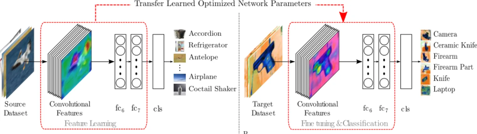
Target Dataset

Fine tuning & Classification Transfer Learned Optimized Network Parameters

A B

Fig. 3: Transfer learning pipeline. (A) shows classification pipeline for a source task, while (B) is a target task, initialized by the parameters learned in the source task.

large datasets are not available gives rise to the concept of transfer learning [35]. The work of [36] illustrated that each hidden layer in a CNN has distinct feature representation related characteristics among of which the lower layers provide general feature extraction capabilities (akin to Gabor filters and alike), while higher layers carry information that is increas-ingly more specific to the original classification task. Figure 2, for instance, demonstrates Gradient-based class activation map (Grad-CAM [30]) of VGG16 [15] for an example X-ray classification object. Lower layers - i.e. conv1−2 and conv2−2, behave as edge detectors, while higher layers like conv4−3 andconv5−3 provides more specific representations

belonging to the input image. This finding facilitates the verbatim re-use of the generalized feature extraction and representation of the lower layers in a CNN, while higher layers are fine-tuned towards secondary problem domains with related characteristics to the original. Using this paradigm, as demonstrated in Figure 3, we can leverage the a priori

CNN parametrization of an existing fully trained network on a generic 1000+ object class problem [42] (Figure 3A), as a starting point for optimization towards to the specific problem domain of limited object class detection within X-ray images (Figure 3B). Instead of designing a new CNN with random weight initialization, we instead adopt a trained CNN, pre-optimized for generalized object recognition, and fine-tune its weights towards our specific classification domain.

C. Application to X-ray Security Imagery

To investigate the applicability of convolutional neural net-works in object classification in X-ray baggage imagery, we address two specific target problems:- a) binary classification problem that performs firearm detection (i.e., gun vs. no-gun) akin to that of the prior work of [4] to compare CNN features to conventional hand crafted attributes; b) a multi-class X-ray object multi-classification problem (6 multi-classes: firearm, firearm-components, knives, ceramic knives, camera and lap-top), which further investigates the performance of CNN for the classification of multiple X-ray objects. The following subsection describes the datasets we use in our experiments.

1) Datasets: To perform classification tasks, we use four

types of datasets described below:

A B C E D F

Fig. 4: Exemplar X-ray baggage image with extracted data set regions including background samples. Type of baggage objects in the dataset is as follows: (A) Firearm Component, (B) Ceramic Knife, (C) Laptop, (D) Camera , (E) Firearm , (F) Knife

Dbp2: Our data-set (11,627 X-ray images) are constructed

using single conventional X-ray imagery with associated false color materials mapping from dual-energy [21]. To generate a dataset for firearm detection, we manually crop baggage objects, and label each accordingly (e.g., Figure 4 ) - on the assumption an in-service detection solution would perform scanning window search through the whole baggage image. In addition to manual cropping, we also generate a set of negative images by randomly selecting256×256fixed-sized overlapping image patches from a large corpus of baggage images that do not contain any target objects. Following these approaches, our evaluation datasets consist of 19,398 X-ray sample patches for a classical two-class firearms detection problem (positive class:3,179firearm images /1,176images of firearm components; negative class:476images of cameras, 2,750 knives, 1,561 ceramic knives, 995 laptops and 9,261 cropped images of background clutter)

Dbp6: For the multiple class problem, we separate firearms

and firearm sub-components into two distinct classes to make the problem even more challenging. Likewise, regular and ceramic knives are considered as two different class objects, which overall we have a 6-class problem for the multi-class task (i.e., each patch being either one of the six object labels). In addition to these datasets, we also use UK government evaluation dataset [19], which is available upon request from UK Home Office Centre for Applied Science and Technology (CAST). This dataset comprises of both expertly concealed

firearm (threat) items and operational benign (non-threat) imagery from commercial X-ray security screening operations on the UK (baggage/parcels). From this dataset, we define two evaluation problems based on the provided annotation for the presence of firearms threat items.

Full Firearm vs. Operational Benign - (FFOB):comprising

4,680 firearm threat and 5,000 non-threat images, and is denoted as FFOB.

Firearm Parts vs. Operational Benign - (FPOB): contains

8,770 firearm and parts threat and 5,000 non-threat images (denoted FPOB, comprising of annotations as any of {bolt carrier assembly, Pump action, Set, Shotgun, Sub-Machine-Gun}).

We split the datasets into training (60%), validation (20%) and test sets (20%) such that each split has similar class distribution but unseen test set contains somewhat challenging samples never trained before. Besides, we also weight the data when sampling to cope with class imbalances. We also perform random flipping, random cropping, and rotation to each sample to augment the datasets.

2) Classification: Using transfer learning paradigm

ex-plained in Section III-B, this work leverages the a priori

CNN parametrization of an existing fully trained network, on a generic 1000 object class problem [42], as a starting point for optimization towards another problem domain of limited object class detection within X-ray images.

For the binary classification problem, we specifically make use of the CNN configuration designed by Krizhevsky et al.

[9], having 5 convolutional layers (conv), 3 fully-connected layers (f c), and trained on the ImageNet dataset on a 1000 class image classification problem, denoted as AlexNet [9].

The first step is to fine tune all of the conv and f c

layers of the network via transfer learning on the training set of the target classification problem. In addition to this, we also perform layer freezing, meaning that instead of updating layer parameters for our task, we use the original unmodified weights from the initial trained CNN parametrization of [9]. This allows us to observe how fine-tuning each layer impacts the overall performance.

Also, having fine-tuned the parameters via this transfer learning approach, we extract the features of the last fully connected layer (f c7) to train on an SVM classifier. This

allows us to additionally compare the internal feature space representation of the CNN model to alternative more tradi-tional (handcrafted) BoVW features as used in prior work [4]. Evaluation of our proposed approach is performed against the prior SVM-driven work of Kundegorski et. al. [4] within a BoVW framework. SVM are trained using Radial Basis Function (RBF) kernel {SV MRBF} with a grid search over kernel parameter, γ = 2x _{: x∈ {−15,3}, and model fitting} cost, c = 2x _{: x ∈ {5,15}, using k-fold cross validation}

(k= 5)with F-score optimization (being more representative then accuracy for unbalanced datasets). The results for the best performing parameter set are reported for each feature configuration.

The second set of experiments is the classification of multiple baggage objects, a more complex six class object problem. Here the lesser performing SVM with handcrafted

features are not considered (Table I), in favor of the CNN approach. Instead, we fine-tune AlexNet [9], VGG [15] and ResNet [16], each of which are top performing entries of ImageNet [42] competition. By doing so, we aim to evaluate the feasibility of CNN for this problem domain further.

To update the parameters of all the networks during training, we use cross-entropy for the loss function, and utilize Adam [44] optimizer with a learning rate of10−3_{, and a weight decay}

of 0.005 since we observe that it achieves superior accuracy to SGD and RMS for this task. Our stopping criterion is to terminate optimization where validation starts to reduce, while training accuracy continues to improve. This fork between training and validation performance usually takes 30 epochs for this task.

D. Evaluation

The performance is evaluated by the comparison of True Positive Rate (TP) (%), False Positive Rate (FP) (%) together with Precision (P), Accuracy (A) and F-score (F) (harmonic mean of precision and true positive rate).

Results for the two class problem is given in Table I, which is divided into four sections: - first section lists the performance of the CNN approach, notated as AlexN etab, meaning that the network is fine-tuned from layer ato layer

b, while the rest of the layers are frozen (Table I, top). This means, for instance, AlexN et4−8 is trained by fine-tuning

the layers{4,5,6,7,8} and freezing the layers{1,2,3} (i.e. remain unchanged from the pre-trained model of [9]). The second section has the results of an SVM classifier trained on the output of the last layer of CNN (Table I, middle upper). Similar to the first section, we again perform layer freezing here for a consistent comparison of CNN features and BoVW features. The third section shows fine tuning results based on contemporary end to end CNN architectures (VGGM [14], VGG16 [15], ResNet18 [16], ResNet50 [16], ResNet101 [16], Table I, middle lower). The last section lists the best performing BoVW feature detector/descriptor variants trained with SVM in the work of [4] (Table I, bottom).

Table I shows the performance results of firearm detection. We see that true and false positives have a general trend to decrease as the number of fine-tuned layers reduces. Likewise, freezing lower layers reduces the accuracy of the models.

Training an SVM classifier on CNN features with layer freezing yields relatively better performance than the standard end to end CNN results. Here, We see a performance pattern such that fine-tuning more layers has a positive impact on the overall performance. For instance, SVM trained on fully fine-tuned CNN has the highest performance on all of the metrics, outperforming the prior work of [4] and [7] (Table I).

For an end to end fine-tuning using contemporary archi-tectures, we observe the direct proportion of performance and network complexity. ResNet101 [16], for instance, is the best performing network among all of the end to end CNN networks (TableI).

It is also significant to note that the performance of the best feature detector/descriptor combination of BoVW approach (FAST/SURF [4]) is worse than any of the CNN features

gun no-gun A camera ceramic-knife gun gun-component knife laptop B

Perplexity: 30 Learning Rate: 135 Iterations: 10000 Perplexity: 40 Learning Rate: 195 Iterations: 10000

Fig. 5: t-SNE [43] visualization of feature maps extracted from the last f clayer of VGG16 [15] fine-tuned for binary (A) and multi-class

(B) problems. TP% FP% P A F A. CNN [9] Layer Freezing AlexNet1-8 99.26 4.08 0.741 0.961 0.849 AlexNet2-8 98.53 2.40 0.832 0.983 0.902 AlexNet3-8 96.32 2.19 0.844 0.980 0.900 AlexNet4-8 95.59 2.96 0.790 0.973 0.865 AlexNet5-8 98.16 4.68 0.711 0.961 0.825 AlexNet6-8 96.32 5.15 0.693 0.954 0.806 AlexNet7-8 94.49 3.65 0.754 0.961 0.839 AlexNet8 95.22 4.21 0.733 0.960 0.828 CNN [9] + SVM Layer Freezing AlexNet1-8 99.56 1.07 0.997 0.994 0.996 AlexNet2-8 99.30 1.50 0.996 0.991 0.994 AlexNet3-8 99.18 1.93 0.995 0.989 0.993 AlexNet4-8 98.92 1.86 0.995 0.988 0.992 AlexNet5-8 98.80 2.07 0.994 0.986 0.991 AlexNet6-8 98.68 3.00 0.991 0.983 0.983 AlexNet7-8 98.64 4.15 0.989 0.980 0.980 AlexNet8 98.42 5.43 0.985 0.976 0.976 CNN End to End VGGM[14] 98.38 0.36 0.998 0.987 0.980 VGG16[15] 99.08 1.14 0.997 0.990 0.985 ResNet18[16] 99.38 1.43 0.996 0.992 0.988 ResNet50[16] 99.54 1.00 0.998 0.995 0.992 ResNet101[16] 99.66 1.14 0.997 0.995 0.993 BoVW SVM [4] SURF/SURF 79.2 3.2 0.88 0.93 0.83 KAZE/KAZE 77.3 3.9 0.85 0.92 0.81 FAST/SURF 83.0 3.3 0.88 0.94 0.85 FAST/SIFT 80.9 4.3 0.85 0.92 0.83 SIFT/SIFT 68.3 4.2 0.83 0.90 0.75

TABLE I: Results of CNN and BoVW on Dbp2 dataset for firearm

detection. AlexNetabdenotes that the network is fine tuned from layer

a to layer b.

given in Table I. Further comparison of BoVW+SVM against CNN+SVM proves the superiority of CNN features to tradi-tional handcrafted features (Table I).

Table II shows the overall performance of the networks fine-tuned for multiple class problem. Like Table I, finetuning the entire network yields the best performance. A conclusion can be reached from these results that fine-tuning higher level layers and freezing lower ones have a detrimental impact on the performance of the CNN model. Similar to Table I, perfor-mance and network complexity are also directly proportional. With relatively lower complexity than the rest, AlexNet [9] has the lowest accuracy of0.924. ResNet101[16], on the other hand, achieves the highest on all metrics (P=96.0%R=96.6%

P R A F AlexNet1-8 0.911 0.904 0.904 0.906 AlexNet2-8 0.842 0.841 0.833 0.835 AlexNet3-8 0.843 0.841 0.844 0.841 AlexNet4-8 0.841 0.853 0.844 0.846 AlexNet5-8 0.833 0.821 0.823 0.811 AlexNet6-8 0.820 0.810 0.819 0.809 AlexNet7-8 0.774 0.793 0.722 0.761 AlexNet8 0.721 0.742 0.701 0.712 VGGM[14] 0.928 0.932 0.923 0.926 VGG16[15] 0.931 0.943 0.940 0.936 ResNet18[16] 0.933 0.943 0.936 0.937 ResNet50[16] 0.934 0.910 0.923 0.917 ResNet101[16] 0.936 0.946 0.937 0.938

TABLE II: Statistical evaluation of CNN architectures (AlexNet, VGG, and ResNet) on Dbp6 dataset for multi-class problem.

TP% FP% P A F AlexNet [9] 99.830 0.943 0.990 0.994 0.994 VGGM[15] 99.010 0.000 1.000 0.995 0.995 VGG16[15] 99.831 0.000 1.000 0.999 0.999 ResNet18[16] 99.472 0.000 1.000 0.997 0.997 ResNet50[16] 100.00 0.923 0.990 0.995 0.995 ResNet101[16] 100.00 0.311 0.996 0.998 0.998

TABLE III: Statistical evaluation of varying CNN architectures (AlexNet, VGG, and ResNet) on FFOB dataset [19].

A=97.5%F=96.1%).

In addition, results are presented on the UK government evaluation dataset [19] in Tables III and IV . Within Table III and IV we present results for classification only (following the approach of Section III-B), where we can see comparable performance to the earlier results presented in Tables I and II.

TP% FP% P A F AlexNet [9] 95.088 3.527 0.960 0.958 0.958 VGGM[15] 95.864 0.919 0.990 0.974 0.974 VGG16[15] 97.238 4.217 0.954 0.965 0.964 ResNet18[16] 95.725 0.744 0.992 0.975 0.974 ResNet50[16] 99.411 1.060 0.988 0.991 0.991 ResNet101[16] 99.608 0.000 1.000 0.998 0.998

TABLE IV: Statistical evaluation of varying CNN architectures (AlexNet, VGG, and ResNet) on FPOB dataset [19].

0.0 0.2 0.4 0.6 0.8 1.0

0: Camera 1: Ceramic Knife 2: Gun 3: Gun Component 4: Knife 5: Laptop

0.98 0.01 0.01 0.0 0.0 0.0 0.0 0.88 0.02 0.02 0.06 0.02 0.0 0.0 0.98 0.02 0.0 0.0 0.0 0.01 0.24 0.74 0.01 0.0 0.0 0.1 0.02 0.02 0.86 0.01 0.0 0.0 0.01 0.0 0.0 0.99 0.99 0.0 0.01 0.0 0.0 0.01 0.01 0.94 0.0 0.02 0.03 0.01 0.0 0.0 0.98 0.01 0.0 0.0 0.01 0.02 0.09 0.86 0.01 0.0 0.0 0.08 0.01 0.01 0.9 0.0 0.0 0.0 0.01 0.0 0.0 0.99 1.0 0.0 0.0 0.0 0.0 0.0 0.0 0.98 0.0 0.0 0.01 0.0 0.0 0.0 0.99 0.01 0.0 0.0 0.01 0.01 0.1 0.88 0.0 0.0 0.0 0.13 0.01 0.01 0.84 0.01 0.0 0.0 0.0 0.0 0.0 1.0 0 1 2 3 4 5 0 1 2 3 4 5 0 1 2 3 4 5 0 1 2 3 4 5 Predicted Label T ru e Lab el AlexNet VGG16 ResNet-101 0 1 2 3 4 5 0 1 2 3 4 5

Fig. 6: Confusion matrices for AlexNet [9], VGG16 [15] ResNet-50 [16] fine tuned for multi class problem

Figure 5 depicts the t-SNE [43] visualization of feature maps of the down-projected internal feature space represen-tation extracted from VGG16 [15] fine-tuned for binary (A) and multi-class (B) problems. In both cases, classes are well separated, showing the capability of CNN features within this problem domain (Figure 5).

Figure 6 depicts per-class accuracy obtained via the use of AlexNet [9] and ResNet101[16], the worst and best performing networks within this task. We see that laptop and camera object classes are straightforward to classify. In contrast, networks have relatively lower classification confidence for knife, ceramic knife vs. firearm, firearm parts, which obviously stems from the similarity of the objects.

Limitations: Due to the cluttered nature of the input dataset,

there are certain cases where CNN based classification fails to classify threats. Figure 7, for instance, demonstrates that CNN labels these image examples as laptops with high confidence, as the predominant object signature present in the image patch, while failing to detect the foreground objects of interest (yellow highlights, Figure 7). This results in a significant increase in false negative occurrences (Table II). We consider this primarily as an object detection problem, and hence explore the contemporary object detection strategies in the subsequent part of this study.

laptop 99.15% laptop 96.43% laptop 97.61%

Fig. 7: Exemplar image cases where CNN (only) classification fails to detect an object in the presence of clutter and other confusing items of interest (here: background laptop detected, knives/guns missed).

IV. OBJECTDETECTION

From Section III, the approach of CNN based classification via transfer learning yields promising performance especially for single and non-occluded X-ray image patches. When it comes to classifying multiple objects (Figure 7), however, more sophisticated approaches are needed to perform joint localization. Here we give a brief introduction to CNN based object detection algorithms for an exhaustive evaluation within X-ray baggage domain.

A. Background

Sermanet et al. (OverFeat) [18] uses a sliding window approach to generate the region proposals, which is then fed into a convolutional neural network for the classification. The key idea here is that bounding box regression is performed with an extra regression layer which shares the weights with the main network. Subsequent work [45] proposes a detec-tion algorithm (RCNN), based on three main stages: region proposal generation, feature extraction, and classification. The first stage employs an external region proposal generator, followed by a fine-tuned CNN in the next stage for feature extraction. The final stage performs classification with an SVM classifier. Even though it outperforms previous work by a large margin, this model is not considered to be real-time applicable due to runtime and memory issues. In contrast, SPPNet [46] contains variable-sized spatial pooling layer between the convolutional and fully connected layers, which allows the network to handle images of arbitrary scales and aspect ratios. With this design, image representations can be computed once in SPPNet, which makes the network significantly faster than RCNN. Like RCNN, however, the network has several separate stages, which is computationally expensive. Fast RCNN by Girshick [47] combines feature extraction, classification and bounding box regression stages by designing a partially end to end CNN network, significantly outperforming [45], [46] regarding speed and accuracy. The novelty of the work is to employ a region of interest pooling layer (RoI) before fully connected layers (f c) to fix the size of the region

proposals generated by the region proposal algorithm. These fixed sized object localization proposals are then classified via f c layers. In addition to the classification, bounding box regression is also performed via a multi-task loss function to localize objects of interests with a bounding rectangle. The limitation, however, is that the network still needs an external region proposal algorithm such as selective search [48]. Inspired by the strong and weak points of [45]–[47],

Ren et al. [11] propose a model, named Faster RCNN

(F-RCNN) performing all the aforementioned stages in an end to end deep neural network. This approach not only reduces time complexity and required memory but also significantly boosts overall performance. Further optimization of this concept by [12] proposes a fully convolutional detection framework (R-FCN), which yields faster training and testing performance with competitive accuracy compared to F-RCNN [11].

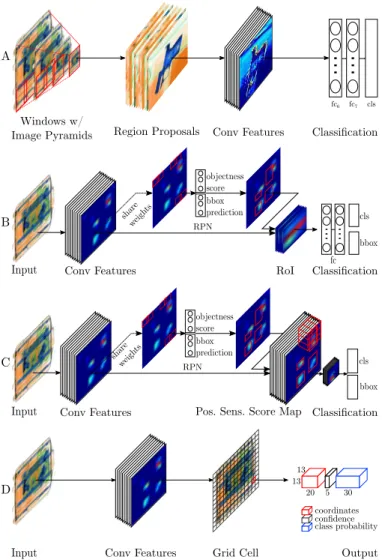
In this work, we adapt F-RCNN, R-FCN and YOLOv2 each of which provide a significant boost in accuracy, for use within an X-ray baggage object detection context, and compare with previous object detection approaches primarily based on traditional sliding window detection frameworks [5], [10].

B. Detection Strategies

Within this work, we consider a number of competing con-temporary detection frameworks and explore their applicability and performance for generalized object detection in X-ray baggage imagery.

Sliding Window Based CNNdetection consists of two main

stages, one of which is to generate objects of interests, while the other one performs classification. To create objects of interest, a fixed sized n ×n window slides over the im-age horizontally and vertically denoting the current region o interest. The disadvantage of using fixed sized window is that large objects may not fit within the window, resulting in weaker proposal generation. The use of image pyramids addresses this issue via the use of multi-scale sampling of the image and subsequent image interpolation of window regions at differing scale to a fixed size classification region input size. First two stages of Figure 8A demonstrate region proposal generation process for a sliding window approach. After generating this region of interest proposals, each is evaluated by the second stage of classification (here using a CNN as per Section III, Figure 8A). As described in Section III, with the use of transfer learning approach, CNN extracts convolutional features and performs classification via fully-connected layers. This method is similar to an external region proposal generator (sliding window traversal of the image) followed by CNN classification.

Faster RCNN (F-RCNN) is based on two subnetworks,

containing a unique region proposal network (RPN) and Fast RCNN network together [11]. Instead of utilizing an external region proposal algorithm as in [45], [47], this model has its region proposal network (the main differentiator from Fast RCNN [47]). The RPN consists of convolutional layers that generate set of anchors with different scales and aspect ratios, and predict their bounding box coordinates together with a probability score denoting whether the region is an object or

Conv Features

Input Grid Cell

13 20 5 30 13 coordinates confidence class probability Output D Classification Input Conv Features

B bbox fc...6 fc...7 cls fc RoI RPN share weigh ts objectness score ... bbox prediction ... ... ... Conv Features Region Proposals A Windows w/

Image Pyramids Classification

fc

...

6 fc

...

7

fc6 fc7 cls

Pos. Sens. Score Map Input Conv Features

C shareweigh RPN ts objectness score ... bbox prediction ... ... ... cls bbox Classification

Fig. 8: Schematics for the CNN driven detection strategies evaluated. A. Sliding Window based CNN (SW-CNN) [4], [7], B. Faster RCNN (F-RCNN) [11], C. R-FCN [12], D. YOLOv2 [13]).

background. Anchors are generated by spatially sliding a 3x3 window through the feature maps of the last convolutional layers of the Fast RCNN network. These features are then fed to objectness classification and bounding box regression layers. Objectness classification layer classifies whether a region proposal is an object or a background while bounding box regression layer predicts the coordinates of the area. An RoI pooling layer resizes these regions to fixed sized dimensions. f c layers then create feature vectors to be used by bounding box regression and softmax layers (see Figure 8B).

R-FCN, proposed by Dai et al. [12], points out the main

limitation of Faster RCNN in that each region proposal within RoI pooling layer is computed numerous of times due to the two subsequent fully connected layers, which is computationally expensive (Figure 8B). They propose a new approach by removing fully-connected layers after RoI pooling, and employing a new variant denoted as “position

sensitive score map”[12], which handles translation variance

issue in detection task (Figure 8C). Removing fully connected subnetworks leads to much faster convergence both in training and test stages, while achieving similar detection performance results to Faster RCNN [11].

YOLOv2 [13] is a fully CNN that achieves state-of-the-art results for object detection. It uses specific techniques to improve its performance against the prior work. Its initial novelty stems from the fact that it performs detection in a single forward-pass, while region-based approaches utilize sub-network for region generation. Like Faster RCNN, it also employs anchors. The main difference here, however, is that instead of fixing the anchor parameters, this approach makes use of k-means clustering over the input data to learn the anchor parameters of the ground truth bounding boxes. In addition to anchors, YOLOv2 performs batch normalization after each layer, resulting in an improvement in the overall per-formance. Another strategy is the use of higher resolution input images together with multi-scale training. Unlike classification networks that inputs smaller size images such as 224×224, YOLOv2 accepts inputs with higher resolution varying be-tween350×350 to600×600. Besides, the model randomly resizes input images during the training, which allows the network to work with objects with varying scales, and hence handles scaling issue. The above strategies yield significant performance improvements, and the approach achieves the state-of-the-art.

The way YOLOv2 works is rather novel. It divides the input into 13×13 grid cells, each of which predicts 5 bounding box coordinates for each anchor. Moreover, for individual predicted bounding boxes, the network outputs confidence score showing the similarity between the bounding boxes and the ground truth. Finally, the output also includes the probability distribution of the classes that the predicted bound-ing boxes belong. Performbound-ing regression and classification within a single network makes YOLOv2 significantly faster, achieving real-time performance.

C. Application to X-ray Security Imagery

We compare four localization strategies for our object detection task within X-ray security imagery: a traditional sliding window approach [10] coupled with CNN classification [18], Faster RCNN (F-RCNN) approach of [11] (a contem-porary architecture within recent object recognition challenge results [42], [49]), R-FCN approach of [12] (comparable to F-RCNN in performance yet offering significant computational efficiency gains over the former), and YOLOv2 [13], which currently achieves the best detection performance on PASCAL VOC benchmark while keeping the computation in real-time.

Dataset: Instead of using multi-view conventional X-ray

patches that we manually crop for the classification task in Section III, here we use full X-ray images to perform binary and multiple class object detection.

Detection: For sliding window CNN (SW-CNN) we employ

800×800 input image, 50×50 fixed size window with a step size of 32 to generate region proposals. We also use image pyramids to fit the window to varying sized objects using 9 pyramid levels. For the classification of the proposed regions we use AlexNet [9], VGGM, 16 [15], and ResNet-{50, 101} [16] networks. Although [18] employs an extra bounding box regression layer within their SW-CNN approach, we do not perform regression as none of the prior work within this domain does so [5], [10].

For Faster RCNN [11] we use the original implementation with a few modifications, and train Faster RCNN with AlexNet [9], VGGM, 16 [15], and ResNet-{50, 101} [16] architectures. Since R-FCN is fully convolutional by design, we only use ResNet-{50, 101} [16] networks for R-FCN to train and test. For the training of the detection strategies explained here, we employ transfer learning approach and use the networks pre-trained on ImageNet dataset [42]. In so doing not only increases performance but also reduces training time sig-nificantly. We use stochastic gradient descent (SGD) with momentum and weight decay of0.9 and0.0005, respectively. The initial learning rate of 0.001 is divided by 10 with step down method in every10,000iteration. For F-RCNN/R-FCN, batch size is set to256 for the RPN. All of the networks are trained by using dual-core Intel Xeon E5-2630 v4 processor and Nvidia GeForce GTX Titan X GPU.

D. Evaluation

Performance of the models is evaluated by mean average precision (mAP), used for PASCAL VOC object detection challenge [50]. To calculate mAP, we perform the following: we first sort nd detections based on their confidence scores. Next, we calculate the area of intersection over union for the given ground truth and detected bounding boxes for each detection as

Ψ(Bgt_i, Bdti) =

Area(Bgti∩Bdti) Area(Bgt_i∪Bdti)

, (1)

whereBgt_i andBdti are ground truth and detected bounding boxes for detection i, respectively. Assuming each detection as unique, and denoting the area as ai, we then threshold it byθ= 0.5 giving a logicalbi, where

bi =

1 ai> θ;

0 otherwise. (2)

This is followed by a prefix-sum giving both true positives~t and false positivesf~, where

ti=ti−1+bi, (3)

fi=ti−1+ (1−bi).

The precisionp~and recall~r curves are calculated as

pi= ti ti+fi , (4) ri= ti np ,

wherenp is the number of positive samples. For a smoother curve, precision vector is then interpolated by using

pi=max(pi, pi+1). (5)

We then calculate average precision (AP) based on the area under precision(~p)recall(~r)curve

AP =

nd

X

i

Model Network mAP camera laptop gun gun component knife ceramic knife SWCNN AlexNet 0.608 0.682 0.609 0.748 0.714 0.212 0.683 VGGM 0.634 0.707 0.637 0.763 0.731 0.246 0.719 VGG16 0.649 0.701 0.724 0.752 0.757 0.223 0.734 ResNet50 0.671 0.692 0.801 0.747 0.761 0.314 0.713 ResNet101 0.776 0.881 0.902 0.831 0.848 0.392 0.803 RCNN AlexNet 0.647 0.791 0.815 0.853 0.582 0.188 0.658 VGGM 0.686 0.799 0.855 0.869 0.658 0.210 0.723 VGG16 0.779 0.888 0.954 0.876 0.832 0.304 0.819 F-RCNN AlexNet 0.788 0.893 0.756 0.914 0.874 0.467 0.823 VGGM 0.823 0.900 0.834 0.918 0.875 0.542 0.869 VGG16 0.883 0.881 0.918 0.927 0.938 0.721 0.912 ResNet50 0.851 0.844 0.879 0.916 0.901 0.677 0.889 ResNet101 0.874 0.857 0.904 0.931 0.911 0.732 0.907 R-FCN ResNet50 0.846 0.894 0.928 0.932 0.918 0.506 0.896 ResNet101 0.856 0.887 0.906 0.942 0.925 0.556 0.920 YOLOv2 Darknet288 0.810 0.821 0.861 0.914 0.904 0.551 0.814 Darknet416 0.851 0.888 0.883 0.952 0.924 0.605 0.851 Darknet544 0.885 0.896 0.894 0.943 0.933 0.728 0.913

TABLE V: Detection results of SW-CNN, Fast-RCNN (F-RCNN) [47], Faster RCNN (F-RCNN) [11], R-FCN [12] and YOLOv2 [13] for multi-class problem (300 region proposals). Class names indicates corresponding average precision (AP) of each class, and mAP indicates mean average precision of the classes.

As shown in Eq 7, we finally find mAP by averaging AP values that we calculate for C classes.

mAP = 1 C C X c=1 APc (7)

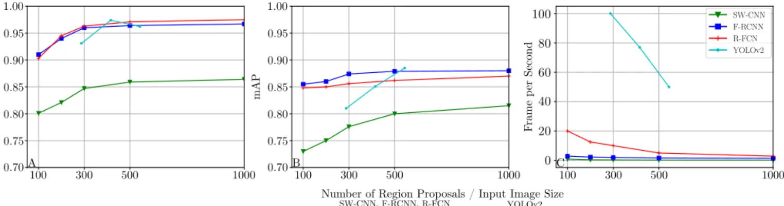
Tables V and VI show binary and multi-class detection results for SW-CNN, F-RCNN, R-FCN with varying networks, and a fixed sized number of region proposals of 300, and for YOLOv2 with a fixed network with varying input image size. For completeness, we additionally present the comparative results for Fast R-CNN (RCNN) [47] (detection architecture pre-dating that of F-RCNN [11] and R-FCN [11]).

As a general trend, we observe that performance increases with overall network complexity such that superior perfor-mance is obtained with VGG16 and ResNet101for the region-based approaches. This observation holds for both the 2-class and 6-2-class problems considered here. Overall, YOLOv2 yields the leading performance for both 2-class and 6-class problems. In addition to this set of experiments, we also train the detection approaches using the pre-trained weights of Dbp6 dataset introduced in Section III-C1. Since not observing significant nuances in results, we do not include them here.

For the multi-class detection task (Table V) we see a similar performance pattern to that seen in the earlier firearm detection task. Here, SW-CNN performs worse than any network trained using a Faster RCNN or R-FCN architecture. Similirwise, overall mAP of RCNN is lower than any FCN and R-FCN architecture. For comparison of F-RCNN and R-R-FCN, we observe that Faster RCNN achieves its highest peak using VGG16, with higher mAP than ResNet-50 and ResNet101. R-FCN with ResNet-50 and ResNet101 yields slightly worse performance, (mAP: 0.846, 0.856) , than that of the best of Faster-RCNN. For the overall performance comparison, YOLOv2 with an input size of 544×544 shows superior performance (mAP:0.885).

For firearm detection Table VI shows that SW-CNN, even with a complex second stage classification CNN such as VGG16 and ResNet101, performs poorly compared to any other detection approaches. This poor performance is primarily due to lacking a bounding box regression layer (Figure 8), a significant performance booster as shown in [18], [45]. Likewise, the best performance of RCNN with VGG16 (mAP: 0.854) is worse than any F-RCNN or R-FCN. This is because the RPN within F-RCNN and R-FCN provides superior object proposals than the selective-search approach used in RCNN. For overall performance on the binary firearm detection task, R-FCN with YOLOv2 with an input image of size 416×416 yields the highest mAP of0.974.

Model Network mAP - firearm SW-CNN AlexNet 0.753 VGGM 0.772 VGG16 0.806 ResNet50 0.836 ResNet101 0.847 RCNN AlexNet 0.823 VGGM 0.836 VGG16 0.854 F-RCNN AlexNet 0.945 VGGM 0.948 VGG16 0.960 ResNet50 0.951 ResNet101 0.960 R-FCN ResNet50 0.949 ResNet101 0.963 YOLOv2 Darknet288 0.931 Darknet416 0.974 Darknet544 0.962

TABLE VI: Detection results of SW-CNN, Fast-RCNN (RCNN) [47], Faster RCNN (F-RCNN) [11], R-FCN [12] and YOLOv2 [13] for firearm detection problem (300 region proposals).

proposals and input image sizes on both detection performance and runtime. Figure 9A-B demonstrate detection performance of the approaches on 2-class and 6-class detection tasks, respectively. Increase in the number of region proposals and input image size lead to a rise in detection performance. Overall, YOLOv2 achieves the highest detection on both tasks. Figure 9C shows mean runtime in frame per second (fps) where we can see YOLOv2 significantly outperforms the rest of the detection approaches. The lowest fps YOLOv2 achieves (50fps) is still considerably better than the best runtime R-FCN (20), F-RCNN (2.9) and SW-CNN (0.8) achieve.

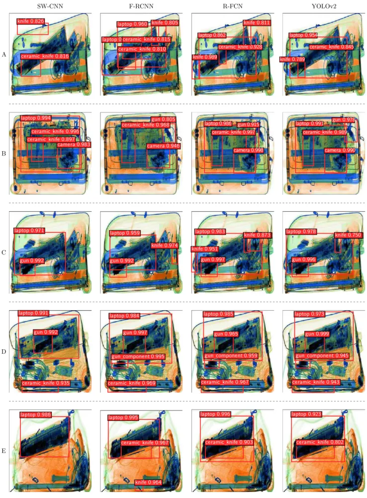
Figure 10 illustrates qualitative examples extracted from the statistical performance analysis of Table V. We see that detection approaches can cope with cluttered datasets where classification methods can fail as shown in Figure 7.

V. CONCLUSION

In this work, we exhaustively explore the use of CNN in the tasks of classification and detection within X-ray baggage imagery. For the classification problem, we make a comparison between CNN and traditional BoVW approaches based on handcrafted features. To do so, we perform layer freezing to observe the relative performance of fixed and fine-tuned sets of CNN feature maps. In addition to this, we train SVM classifier on top of the last layer of the network to have a consistent comparison between CNN and handcrafted features. We also explore various CNN to see the impact of network complexity on overall performance.

Experimentation demonstrates that CNN features achieve superior performance to handcrafted BoVW features. Fine tuning the entire network for this problem yields 0.996% True Positive (TP),0.011False Positive (FP) and0.994 accu-racy (A), a significant improvement on the best performing handcrafted feature detector/descriptor (FAST/SURF, 0.830 TP, 0.033 FP,0.940 A). For the classification of multiple X-ray baggage objects, ResNet-50 achieves 0.986 (A), clearly demonstrating the applicability of CNN within X-ray baggage imagery, and outperforming prior reported results in the field [1]–[5].

In addition to classification, we also study object detection strategies to improve the performance of cluttered datasets further, where classification techniques fail. Hence, we ex-amine the relative performance of traditional sliding window driven detection with CNN model [10], [18] against contem-porary region-based [11], [12], [47] and single forward-pass based [13] CNN variants. We show that contemporary Faster RCNN, R-FCN, and YOLOv2 approaches outperform SW-CNN, which is already empirically shown to outperform hand-crafted features, regarding both speed and accuracy. YOLOv2 yields0.885and0.974mAP over 6-class object detection and 2-class firearm detection problems, respectively. This result illustrates the real-time applicability and superiority of such integrated region based detection models within this X-ray security imagery context.

Future work will consider exploiting multi-view X-ray se-curity imagery in an end to end design.

ACKNOWLEDGMENT

The authors would like to thank the UK Home Office for partially funding this work. Views contained within this paper are not necessarily those of the UK Home Office.

REFERENCES

[1] M. Ba¸stan, M. R. Yousefi, and T. M. Breuel, Visual Words on Baggage X-Ray Images. Berlin, Heidelberg: Springer Berlin Heidelberg, 2011, pp. 360–368. [Online]. Available: http://dx.doi.org/ 10.1007/978-3-642-23672-3_44 1, 2, 3, 11

[2] D. Turcsany, A. Mouton, and T. P. Breckon, “Improving feature-based object recognition for x-ray baggage security screening using primed visualwords,” in2013 IEEE International Conference on Industrial Technology, Feb 2013, pp. 1140–1145. 1, 2, 3, 11

[3] M. Bastan, W. Byeon, and T. M. Breuel, “Object recognition in multi-view dual energy x-ray images,” inBMVC, 2013. 1, 2, 11

[4] M. Kundegorski, S. Akçay, M. Devereux, A. Mouton, and T. P. Breckon, “On using feature descriptors as visual words for object detection within x-ray baggage security screening,” in International Conference on Imaging for Crime Detection and Prevention], IET (November 2016). 1, 2, 3, 4, 5, 6, 8, 11

[5] M. Ba¸stan, “Multi-view object detection in dual-energy x-ray images,” Machine Vision and Applications, vol. 26, no. 7-8, pp. 1045–1060, 2015. 1, 2, 8, 9, 11

[6] D. Mery, E. Svec, and M. Arias, Object Recognition in Baggage Inspection Using Adaptive Sparse Representations of X-ray Images. Cham: Springer International Publishing, 2016, pp. 709–720. [Online]. Available: http://dx.doi.org/10.1007/978-3-319-29451-3_56 1, 2, 3 [7] S. Akçay, M. E. Kundegorski, M. Devereux, and T. P. Breckon, “Transfer

learning using convolutional neural networks for object classification within x-ray baggage security imagery,” inImage Processing (ICIP), 2016 IEEE International Conference on. IEEE, 2016, pp. 1057–1061. 1, 2, 3, 5, 8

[8] D. Mery, E. Svec, M. Arias, V. Riffo, J. M. Saavedra, and S. Banerjee, “Modern computer vision techniques for x-ray testing in baggage inspection,”IEEE Transactions on Systems, Man, and Cybernetics: Systems, vol. 47, no. 4, pp. 682–692, 2017. 1, 2, 3

[9] A. Krizhevsky, I. Sutskever, and G. E. Hinton, “Imagenet classification with deep convolutional neural networks,” in Advances in neural information processing systems, 2012, pp. 1097–1105. 1, 2, 3, 5, 6, 7, 9

[10] T. Franzel, U. Schmidt, and S. Roth,Object detection in multi-view X-ray images. Springer, 2012, pp. 144–154. 1, 2, 8, 9, 11

[11] S. Ren, K. He, R. Girshick, and J. Sun, “Faster r-cnn: Towards real-time object detection with region proposal networks,” inAdvances in neural information processing systems, 2015, pp. 91–99. 1, 2, 3, 8, 9, 10, 11 [12] J. Dai, Y. Li, K. He, and J. Sun, “R-FCN: object detection via region-based fully convolutional networks,”CoRR, vol. abs/1605.06409, 2016. [Online]. Available: http://arxiv.org/abs/1605.06409 1, 2, 3, 8, 9, 10, 11 [13] J. Redmon and A. Farhadi, “YOLO9000: Better, Faster, Stronger,”

ArXiv e-prints, Dec. 2016. 1, 3, 8, 9, 10, 11

[14] K. Chatfield, K. Simonyan, A. Vedaldi, and A. Zisserman, “Return of the devil in the details: Delving deep into convolutional nets,”CoRR, vol. abs/1405.3531, 2014. [Online]. Available: http://arxiv.org/abs/1405.3531 2, 3, 5, 6

[15] K. Simonyan and A. Zisserman, “Very deep convolutional networks for large-scale image recognition,” CoRR, vol. abs/1409.1556, 2014. [Online]. Available: http://arxiv.org/abs/1409.1556 2, 3, 4, 5, 6, 7, 9 [16] K. He, X. Zhang, S. Ren, and J. Sun, “Deep residual learning for image

recognition,” inProceedings of the IEEE Conference on Computer Vision and Pattern Recognition, 2016, pp. 770–778. 2, 3, 5, 6, 7, 9 [17] D. Mery, V. Riffo, I. Zuccar, and C. Pieringer, “Object recognition in

x-ray testing using an efficient search algorithm in multiple views,” Insight-Non-Destructive Testing and Condition Monitoring, vol. 59, no. 2, pp. 85–92, 2017. 2, 3

[18] P. Sermanet, D. Eigen, X. Zhang, M. Mathieu, R. Fergus, and Y. LeCun, “Overfeat: Integrated recognition, localization and detection using convolutional networks,” CoRR, vol. abs/1312.6229, 2013. [Online]. Available: http://arxiv.org/abs/1312.6229 2, 7, 9, 10, 11 [19] “OSCT Borders X-ray Image Library, UK Home Office Centre for

Applied Science and Technology (CAST),” Publication Number: 146/16, 2016. [Online]. Available: https://www.gov.uk/government/collections/ centre-for-applied-science-and-technology-information 2, 4, 6

Number of Region Proposals / Input Image Size SW-CNN, F-RCNN, R-FCN YOLOv2 100 300 500 1000 1.00 0.95 0.90 0.85 0.80 0.75 0.70 mAP 100 300 500 1000 1.00 0.95 0.90 0.85 0.80 0.75 0.70 mAP 100 300 500 1000 Frame p er Second 100 80 60 40 20 0 A B C

Fig. 9: Impact of number of box proposals on performance. (A) for binary class (B) for multi-class (C) Runtime. Models are trained using ResNet101

[20] S. Singh and M. Singh, “Explosives detection systems (eds) for aviation security,”Signal Processing, vol. 83, no. 1, pp. 31–55, 2003. 2 [21] A. Mouton and T. P. Breckon, “A review of automated image

under-standing within 3D baggage computed tomography security screening,” Journal of X-ray science and technology, vol. 23, no. 5, pp. 531–555, 2015. 2, 3, 4

[22] T. W. Rogers, N. Jaccard, E. J. Morton, and L. D. Griffin, “Automated x-ray image analysis for cargo security: Critical review and future promise,”Journal of X-ray science and technology, vol. 25, no. 1, pp. 33–56, 2017. 2, 3

[23] Z. Chen, Y. Zheng, B. R. Abidi, D. L. Page, and M. A. Abidi, “A combinational approach to the fusion, de-noising and enhancement of dual-energy x-ray luggage images,” inComputer Vision and Pattern Recognition-Workshops, 2005. IEEE Computer Society Conference On. IEEE, 2005, pp. 2–2. 2

[24] B. R. Abidi, Y. Zheng, A. V. Gribok, and M. A. Abidi, “Improving weapon detection in single energy x-ray images through pseudocolor-ing,”IEEE Transactions on Systems, Man, and Cybernetics, Part C (Applications and Reviews), vol. 36, no. 6, pp. 784–796, 2006. 2 [25] Q. Lu and R. W. Conners, “Using image processing methods to improve

the explosive detection accuracy,” IEEE Transactions on Systems, Man, and Cybernetics, Part C (Applications and Reviews), vol. 36, no. 6, pp. 750–760, 2006. 2

[26] M. Singh and S. Singh, “Image segmentation optimisation for x-ray images of airline luggage,” in Computational Intelligence for Homeland Security and Personal Safety, 2004. Proceedings of the 2004 IEEE International Conference on. IEEE, 2004, pp. 10–17. 2 [27] G. Heitz and G. Chechik, “Object separation in x-ray image sets,” in Computer Vision and Pattern Recognition, 2010 IEEE Conference on. IEEE, 2010, pp. 2093–2100. 2

[28] D. Mery, “Automated detection in complex objects using a tracking algorithm in multiple x-ray views,” inComputer Vision and Pattern Recognition Workshops, 2011 IEEE Computer Society Conference on. IEEE, 2011, pp. 41–48. 2

[29] L. Schmidt-Hackenberg, M. R. Yousefi, and T. M. Breuel, “Visual cortex inspired features for object detection in x-ray images,” inPattern Recognition, 2012 21st International Conference on. IEEE, 2012, pp. 2573–2576. 2

[30] R. R. Selvaraju, A. Das, R. Vedantam, M. Cogswell, D. Parikh, and D. Batra, “Grad-cam: Why did you say that? visual explanations from deep networks via gradient-based localization,” CoRR, vol. abs/1610.02391, 2016. [Online]. Available: http://arxiv.org/abs/1610. 02391 3, 4

[31] N. Dalal and B. Triggs, “Histograms of oriented gradients for human detection,” inComputer Vision and Pattern Recognition, 2005. CVPR 2005. IEEE Computer Society Conference on, vol. 1. IEEE, 2005, pp. 886–893. 2

[32] G. Flitton, T. P. Breckon, and N. Megherbi, “A comparison of 3D interest point descriptors with application to airport baggage object detection in complex CT imagery,”Pattern Recognition, vol. 46, no. 9, pp. 2420– 2436, 2013. 3

[33] G. Flitton, A. Mouton, and T. P. Breckon, “Object classification in 3D baggage security computed tomography imagery using visual code-books,”Pattern Recognition, vol. 48, no. 8, pp. 2489–2499, 2015. 3 [34] A. Mouton and T. P. Breckon, “Materials-based 3D segmentation of

unknown objects from dual-energy computed tomography imagery in baggage security screening,”Pattern Recognition, vol. 48, no. 6, pp. 1961–1978, 2015. 3

[35] M. Oquab, L. Bottou, I. Laptev, and J. Sivic, “Learning and transferring mid-level image representations using convolutional neural networks,” in Proceedings of the IEEE conference on computer vision and pattern recognition, 2014, pp. 1717–1724. 3, 4

[36] J. Yosinski, J. Clune, Y. Bengio, and H. Lipson, “How transferable are features in deep neural networks?” inAdvances in neural information processing systems, 2014, pp. 3320–3328. 3, 4

[37] C. Szegedy, W. Liu, Y. Jia, P. Sermanet, S. Reed, D. Anguelov, D. Erhan, V. Vanhoucke, and A. Rabinovich, “Going deeper with convolutions,” CoRR, vol. abs/1409.4842, 2014. [Online]. Available: http://arxiv.org/abs/1409.4842 3

[38] V. Badrinarayanan, A. Kendall, and R. Cipolla, “Segnet: A deep convolutional encoder-decoder architecture for image segmentation,” CoRR, vol. abs/1511.00561, 2015. [Online]. Available: http://arxiv.org/ abs/1511.00561 3

[39] Y. Lecun, L. Bottou, Y. Bengio, and P. Haffner, “Gradient-based learning applied to document recognition,”Proc of the IEEE, vol. 86, no. 11, pp. 2278–2324, Nov 1998. 3

[40] M. D. Zeiler and R. Fergus, “Visualizing and understanding convolutional networks,” CoRR, vol. abs/1311.2901, 2013. [Online]. Available: http://arxiv.org/abs/1311.2901 3

[41] C. Szegedy, V. Vanhoucke, S., J. Shlens, and Z. Wojna, “Rethinking the inception architecture for computer vision,”CoRR, vol. abs/1512.00567, 2015. [Online]. Available: http://arxiv.org/abs/1512.00567 3

[42] O. Russakovsky, J. Deng, H. Su, J. Krause, S. Satheesh, S. Ma, Z. Huang, A. Karpathy, A. Khosla, M. Bernsteinet al., “Imagenet large scale visual recognition challenge,”International Journal of Computer Vision, vol. 115, no. 3, pp. 211–252, 2015. 3, 4, 5, 9

[43] L. v. d. Maaten and G. Hinton, “Visualizing data using t-sne,”Journal of Machine Learning Research, vol. 9, no. Nov, pp. 2579–2605, 2008. 6, 7

[44] D. P. Kingma and J. Ba, “Adam: A method for stochastic optimization,” CoRR, vol. abs/1412.6980, 2014. [Online]. Available: http://arxiv.org/abs/1412.6980 5

[45] R. Girshick, J. Donahue, T. Darrell, and J. Malik, “Rich feature hierarchies for accurate object detection and semantic segmentation,” in Proceedings of the IEEE conference on computer vision and pattern recognition, 2014, pp. 580–587. 7, 8, 10

[46] K. He, X. Zhang, S. Ren, and J. Sun, “Spatial pyramid pooling in deep convolutional networks for visual recognition,” CoRR, vol. abs/1406.4729, 2014. [Online]. Available: http://arxiv.org/abs/1406.4729 7, 8

[47] R. B. Girshick, “Fast R-CNN,” CoRR, vol. abs/1504.08083, 2015. [Online]. Available: http://arxiv.org/abs/1504.08083 7, 8, 10, 11 [48] J. R. Uijlings, K. E. Van De Sande, T. Gevers, and A. W. Smeulders,

“Selective search for object recognition,” International journal of computer vision, vol. 104, no. 2, pp. 154–171, 2013. 8

[49] T. Lin, M. Maire, S. Belongie, J. Hays, P. Perona, D. Ramanan, P. Dollár, and C. L. Zitnick,Microsoft COCO: Common Objects in Context. Cham: Springer International Publishing, 2014, pp. 740–755. [Online]. Available: http://dx.doi.org/10.1007/978-3-319-10602-1_48 9 [50] M. Everingham, L. Van Gool, C. K. Williams, J. Winn, and A. Zisser-man, “The pascal visual object classes (voc) challenge,”International journal of computer vision, vol. 88, no. 2, pp. 303–338, 2010. 9

A B C D E knife 0.826 ceramic_knife 0.816 camera 0.983 laptop 0.994 ceramic_knife 0.996 ceramic_knife 0.897 laptop 0.971 gun 0.992 laptop 0.991 gun 0.992 ceramic_knife 0.935 laptop 0.986 SW-CNN laptop 0.960 laptop 0.848 knife 0.805 ceramic_knife 0.815 ceramic_knife 0.810 camera 0.946 gun 0.805 ceramic_knife 0.968 laptop 0.959 gun 0.992 knife 0.974 laptop 0.984 gun 0.997 gun_component 0.995 ceramic_knife 0.969 laptop 0.995 knife 0.964 ceramic_knife 0.967 F-RCNN laptop 0.862 knife 0.989 ceramic_knife 0.928 camera 0.998 laptop 0.986 gun 0.915 ceramic_knife 0.997 laptop 0.983 gun 0.997 gun 0.830 knife 0.951 knife 0.873 laptop 0.985 gun 0.965 gun_component 0.959 ceramic_knife 0.967 laptop 0.996 ceramic_knife 0.903 R-FCN laptop 0.954 knife 0.789 ceramic_knife 0.845 camera 0.990 laptop 0.991 gun 0.978 ceramic_knife 0.989 laptop 0.978 gun 0,996 gun 0.830 knife 0.750 laptop 0.973 gun 0.999 gun_component 0.945 ceramic_knife 0.943 laptop 0.923 ceramic_knife 0.802 YOLOv2 knife 0.811