Dynamic Feature Selection for
Clustering High Dimensional Data
Streams
CONOR FAHY1, SHENGXIANG YANG12(Senior Member, IEEE)
1Centre for Computational Intelligence (CCI), School of Computer Science and Informatics, De Montfort University, The Gateway, Leicester LE1 9BH, U.K. 2Department of Computer Science and Engineering, Southern University of Science and Technology, Shenzhen 518055, China
Corresponding author: Shengxiang Yang (e-mail: [email protected]).
“This work was supported in part by the National Natural Science Foundation of China (NSFC) under Grant 61673331 and Shenzhen Peacock Plan under grant KQTD2016112514355531.”
ABSTRACT Change in a data stream can occur at the concept level and at the feature level. Change at the feature level can occur if new, additional features appear in the stream or if the importance and relevance of a feature changes as the stream progresses. This type of change has not received as much attention as concept-level change. Furthermore, a lot of the methods proposed for clustering streams (density-based, graph-based, grid-based) rely on some form of distance as a similarity metric and this is problematic in high-dimensional data where the curse of dimensionality renders distance measurements and any concept of ‘density’ difficult. To address these two challenges we propose combining them and framing the problem as a feature selection problem, specifically adynamicfeature selection problem. We propose a Dynamic Feature Mask for clustering high dimensional data streams. Redundant features are masked and clustering is performed along unmasked, relevant features. If a feature’s perceived importance changes, the mask is updated accordingly; previously unimportant features are unmasked and features which lose relevance become masked. The proposed method is algorithm-independent and can be used with any of the existing density based clustering algorithms which typically do not have a mechanism for dealing with feature drift and struggle with high-dimensional data. We evaluate the proposed method on four density-based clustering algorithms across four high-dimensional streams; two text streams and two image streams. In each case, the proposed Dynamic Feature Mask improves clustering performance and reduces the processing time required by the underlying algorithm. Furthermore, change at the feature level can be observed and tracked.
INDEX TERMS Data Stream Clustering, Dynamic Feature Selection, Feature Drift, Feature Evolution, High Dimensional Data Streams, Unsupervised Feature Selection
I. INTRODUCTION
A
LONG with time and memory constraints, change is an important consideration in data stream mining. Recog-nising and reacting to change is important for accurate, real-time analysis. Change in a stream can happen in a number of ways. Let S = [xt]∞t=0 denote a stream where x is a
vector inddimensions at timet. LetY represent the set ofk
discovered clusters:Y ={y1, . . . , yk}. We can represent the
assignment of a pointxito a clusteryj∈Y as a conditional
probabilityPt(y
j|xi); the probability of xi belonging to a
clusteryj at timet. One possible type of change is concept
evolution. Concept evolution occurs when an entirely new clusterymappears in the stream,ym 6∈ Y. Another type of
change in a data stream can occur in the form of concept drift.
This occurs if the characteristics of the data change, i.e., if the underlying process generatingxchanges. Typically, this kind of drift is referred to as virtual drift, a change inPt(x).
A second type of drift is known as real drift, a change in
Pt(y|x). For example, at timetpointxiis assigned to cluster yj, but att+δ,xiis assigned to clusterym. This would occur
if, for example, clustersyjandymhave drifted into different
positions in the feature space.
A third type of change which has not received as much attention is a change at the feature level. Change at the feature level can occur in two ways; feature drift and feature evolution. Assuming an incoming instancexinddimensions
x = {f1, . . . , fd}. Feature drift occurs if the importance,
discriminatory power or relevance of a feature fi changes
over the course of a stream. For example, in text-mining the relevance of a particular word can change over time. Feature evolution occurs when new features appear in the stream, for example, additional words might appear in a text stream and
d, the dimensionality ofx, changes.
A lot of attention has been given to clustering streams in the presence of change at the concept level but very little to change at the feature level. Furthermore, a lot of the methods proposed for clustering streams (density-based, graph-based) rely on distance as a similarity metric and this is problematic for high-dimensional data where the curse of dimensionality renders distance measurements and any concept of ‘density’ difficult. To address these two challenges we propose com-bining them and framing the problem as a feature selection problem.
Feature selection (FS) aims to identify a subset of the most relevant features fˆfrom the set of all features F (In this work, ‘feature’ and ‘dimension’ can be used interchange-ably). Traditionally,fˆwould be used to cluster data and all redundant features ({fi : fi ∈ F andfi ∈/ fˆ}) are ignored
for future points. This might not be a sensible approach to non-stationary data as fˆ is likely to change over time. A significant change could require previous clusters to be abandoned and new clusters discovered on the latest data. This would be especially true for clustering algorithms that rely on some form of distance as a similarity metric; it might not be possible to cluster two points composed of different feature subsets, e.g., if the number of ‘important’ features changes (|fˆt| 6=|fˆt+1|) or a previously important feature is
no longer considered important (fi ∈fˆtbutfi∈/ftˆ+1)).
Motivated by these challenges we propose using a dynamic feature mask for clustering high dimensional data streams. A stream is split into windows of sizeβ and unsupervised FS is performed after each window. Redundant features are masked and clustering is performed along unmasked, rele-vant features. If a feature’s perceived importance changes, the mask is updated accordingly - previously unimportant features can be unmasked and features which lose relevance become masked. As new features appear in the stream, the size of the mask is changed. Clustered points contain all fea-tures (not just a subset of relevant feafea-tures) but the clustering process only considers the subset of relevant features.
In summary, we propose a novel Dynamic Feature Mask method for clustering high dimensional data streams and the main contributions of this work are:
• Feature Drift and Feature Evolution can be detected and tracked in a fully unsupervised way and the importance of features can be monitored over time.
• The method is algorithm-independent and can be used
with any of the existing density-based stream clustering algorithms which typically do not have a feature drift mechanism and are unable to deal with high dimension-al data.
• Applied to an existing stream clustering algorithm, the proposed method can reduce the time requirements and increase accuracy.
We offer an overview of related work in Section II along with a more detailed description of relevant background work in Section III. The proposed method is presented in Section IV. Experimental results are described in Section V. Finally, conclusions are given in Section VI.
II. RELATED WORK
Much research has been carried out on Feature Selection (FS) and good overviews on this research are available in [37] and [2]. The majority of this research has focused onsupervised
methods, whereby a feature’s importance is estimated by its correlation with the class label. Features (or subsets of features) with the greatest discriminatory power between classes are selected. Generally, FS methods can be divided into filter methods and wrapper methods. Filter methods are independent of the model and can be seen as a preprocessing step which rank features according to some criterion and the top n features are selected. Popular methods include the Fisher Score [25], Information Gain [36] and Pearson Coefficient [11]. Wrapper methods use a model or an under-lying classifier to iteratively evaluate subsets of features. An example would be the GA-SVM [29], a genetic algorithm searches for subsets of features and these potential subsets are evaluated using a traditional support vector machine.
Unsupervised methods, too, can be divided into filter and wrapper methods. Unsupervised wrapper techniques use a clustering algorithm to evaluate feature subsets [35]. This method is usually computationally expensive and succumbs to what Alelyani et al. described as the “Chicken and Egg Dilemma” [2]. When attempting to cluster and select features simultaneously, is it better to first find features and then cluster, or first cluster and then select features?
Unsupervised filter methods are based on the intrinsic properties of the data, for example, the assumption that data from the same class are usually close in the decision space. Based on this assumption, features are selected by their locality preserving power, or Laplacian Score. This idea has been applied for unsupervised FS in [9] and is explained in detail in Section III. Infinite-Feature Selection [44] selects features by exploiting the convergence properties of power series of matrices. A subset of features is analogous to a path between different feature distributions. In [13], the authors propose a filter method which selects features based on their ability to preserve the original structure of the data. Their algorithm, Multi-Cluster Feature Selection (MCFS), measures the correlation between different features using spectral analysis techniques and selects those which can most preserve the structure. This algorithm is explained in greater detail in Section III.
Most of the research into FS has assumed a static batch of data but recently more work has been focusing on FS in streaming data. A comprehensive overview of this recent work is provided in [4]. Again, the majority of this research has been on supervised FS. The work by Katakis et al. [33] was one of the first to address the FS problem in streaming data. Here, the authors address the problem of a
large, dynamic feature space. They use the example of a text stream, the feature space being all possible words. As more text arrives, new words (features) appear and the size of the known feature space grows and changes. Cumulative statistics based on the word count in each class of document are recorded. Using the chi-squared metric the topnwords in each document are selected as inputs for a Naive-Bayes clas-sifier. As a new document arrives, the cumulative statistics are updated. Features can be promoted or demoted from the top nand the classifier is updated with these new features. Heterogeneous Ensemble for Feature Drift (HEFT) [42] uses a Fast Correlation Based Filter [27] as a supervised filter method to select the top features in each windowed chunk of a data stream. A classifier is trained using the top features and added to an ensemble where each classifier is trained on a different feature subset. Carvalho et al. [15] used the weights of an online classifier to estimate the importance of each feature. Interestingly, the authors found that using some of the lowest ranked features improved the classification accuracy. The authors report using 90% of the top features and 10% of the bottom features.
Feature Selection based on Symmetric Uncertainty (a con-cept taken from Information Theory) was introduced in [7] and extended in [5] with Dynamic Symmetrical Uncertainty Selection for Streams (DISCUSS). DISCUSS is classifier independent and acts as a filter method in a sliding window. Features are selected using a merit-guided strategy whereby the perceived merit of a subset of features is a function of how predictive of a class the subset is, and also how much redundancy there is within the subset. This selection method was shown to improve the performance of two different types of classifiers. Adaptive Boosting for FS (ABFS) was introduced by Barddalet al.[6] and uses a combination of boosting [23] and decision stumps (a decision tree whereby the root node is connected to the terminal nodes) to select features. Boosting gives higher weights to training instances which are harder to classify, then decision stumps are used to select features from these difficult-to-classify samples. ABFS is shown to improve classification rates while also reduc-ing computational overheads. Other supervised approaches dynamically select features implicitly [12], [24]. DX-Miner [40] is a streaming classification algorithm that incorporates dynamic FS. The algorithm can use either a supervised or an unsupervised filter method. For the supervised method, the previous three windows are stored and the Information Gain metric is used to select the top features from these recent windows. In the unsupervised case, the authors suggest that thenhighest frequency features could be used but this is not discussed any further. This was extended in [46], here the authors used DX-Miner with MCFS as the filter method. An unsupervised FS method for data streams with linear time and space was proposed in [30]. Matrix sketching is used to maintain a low rank approximation of the data. At every time-stept, the top features are selected, thoughalldata until time
tis used for selecting the top features. The authors reported that this gave memory problems with comparative algorithms
and in a dynamic stream it is perhaps better to disregard data as the stream progresses and old data is no longer relevant.
Other work in feature processing is concerned with the task ofcreatingnew features (as opposed to selecting) from the existing set of features [38], [39], [49]. In [49] a Deep Neural Network is developed to detect spoofing in an auto-matic Speaker Verification System and the paper reports that selecting features dynamically works more effectively that static selection.
Clustering data streams differs from traditional clustering. There are additional time and memory constraints, usually only a single pass of the data is afforded, and some form of change is expected. Many approaches have been pro-posed including grid based methods [10], [45] and partitional methods [26], although Density Based methods appear to be the most common. Density clustering methods [17] identify clusters as areas of high density separated by areas of low density. They have the advantages that the number of clusters does not need to be specified a-priori, clusters can have any shape (not just hyper-spherical), and they can have an intrinsic summarisation method; the micro-cluster. Micro-clusters ared-dimensional spheres which summarise a group of local points. The set of connected micro-clusters form the cluster. CluStream [1] was one of the first to employ micro-clusters to cluster dynamic data streams. A two-phase approach was proposed, whereby data is first summarised online and the summaries are then clustered off-line. This two-phase approach was extended in MR-Stream [47], D-Stream [45], DenD-Stream [14], and others. A good overview on density based stream clustering is provided in [3]. More recent proposals for density-clustering include Ant Colony Stream clustering (ACSC) [19], which uses a decentralised swarm intelligence approach, CEDAS [31] and SNCStream+ [8], use a graph structure with micro-clusters as nodes, and Multi-Density Stream Clustering (MDSC) [20], which com-bines both online and off-line phases into a single online phase and can discover clusters with varying levels of density. In summary, the majority of research on dynamic FS for data streams assume the supervised method [15], [33], [40], [42] and is typically used for classification tasks and not suitable for clustering. Existing stream-clustering algorithms can deal with change at the concept level (concept drift and concept evolution) [14], [19], [20], [31]. However, these methods suffer from the curse of dimensionality and are not designed to track change at the feature level. The method proposed in this paper aims to address these two challenges: tracking change at the feature level and dynamically cluster-ing in high dimensions.
III. BACKGROUND
The proposed method requires an unsupervised feature selec-tor. We evaluate three existingstaticmethods for maintaining the dynamicfeature mask. Each method is described below along with the clustering algorithms we use to evaluate the proposed dynamic feature mask.
A. UNSUPERVISED FEATURE SELECTION
1) Variance
The most simple, yet effective, method of unsupervised feature selection is the maximum-variance method; the av-erage squared deviation of a feature’s value from the mean.
X ={x1, . . . , xN}representsNinstances, wherexi ∈Rd: V ar(Xi) = 1 N N X j=1 (Xij−µi)2 (1)
A larger variance suggests the feature has a greater repre-sentative power. The intuition here is that if a feature does not vary much (if it has a near constant relevance for each different class) it has little predictive power. However, if a feature is sufficiently different for each class it is potentially more useful when discriminating between classes.
The variance for each feature is calculated, the features are ranked in the descending order, and top n features are selected.
2) Lapacian Score
The Lapacian Score [9] aims to preserve the local geometric structure in data. This local structure is modelled in a nearest-neighbour graph and features which respect this graph are selected.
• A nearest-neighbour graphGis created withN nodes and an edge is created between nodesiandjifxiandxj
are neighbours (xiis amongxj’sknearest neighbours
or vice versa).
• A weight matrixSofGmodels the local structure. An
RBF function with a constantt∈Ris used to weigh the edge between nodesiandj:
Sij = (
e−k(xi−xj)k2 1t : ifiandjare neighbours
0 : otherwise
(2)
• The importance of a feature is considered to be the degree to which it respects G and the weight matrix
S. The Lapacian ScoreLfor featurefris estimated by
minimising: Lr= P ij(fri−frj) 2S ij V ar(fr) (3) A good feature will have a largerSij(thus a smallerfri−frj)
and should have a high variance. So, the Lapacian Score for a good feature should be small. The Lapacian Score for each feature is calculated, the features are ranked in the ascending order, and topnfeatures are selected.
3) Multi Cluster Feature Selection (MCFS)
MCFS [13] uses spectral clustering to select the features which have the most structure-preserving power. Spectral clustering is performed using the top eigenvectors of the graph Lapacian. As in the Lapacian Score, a nearest neigh-bour graphGand weight matrixSare created. The data man-ifold inS is “unfolded” to a “flat” embedding of data points
and features are selected using the “flat” embedding. From
S, a diagonal matrixD is created whose values are column sums of S;Dij = PjSij. From these matrices, the graph
LapacianL = D−W is created and the “flat” embedding of the data can be found by solving the generalised eigen-problem:
Ly=λDy (4)
The feature scores are evaluated using the resultant eigen-vectorsY ={Y1, . . . , Yk}, wherekis the number of clusters
in the data. In static batch data, kmight be known a-priori, or can be tuned to find the best solution. In the streaming case,kcan not be known. So, we use the number of clusters discovered in thepreviouswindow.
MCFS scores for each feature are sorted in the descending order and the topnare selected.
B. STREAM CLUSTERING ALGORITHMS
To evaluate our proposed method, we use four density based stream clustering algorithms; MDSC [20], ACSC [19], CEDAS [31] and DenStream [14]. Clusters are defined as areas of high density separated by areas of low density. Points which are close in the feature space (measured using the Euclidean distance) are summarised in micro-clusters.
A micro-cluster containingNpoints{X~j},j={1, ..., N},
is described using four components: N, the number of points described by the micro-cluster, each of which is an d -dimensional vector; LS, the linear sum of these points (i.e.,
N P j=1
~
Xj); SS, the squared sum of these points (i.e., N P j=1 ~ X2 j);
andt, the time stamp.
LS and SS are d-dimensional vectors. From these three components, we can obtain the centrec and radiusrof the micro-cluster as follows: c= LS N (5) r= s SS N − LS N 2 (6) The time stamptrecords the most recent time a micro-cluster was updated (in CEDAS, the time stamp is referred as the ‘energy’ of the micro-cluster).
The concept of ‘dense’ is governed by a parameter , which is the maximum radius allowed for a micro-cluster. It is sensitive and data-dependant. This is a user-parameter in ACSC and CEDAS, but MDSC discovers this parameter adaptively, removing a sensitive, manually tuned parameter. Two micro-clustersaandbare considered density reachable if:
dist(acen, bcen)≤ar+br. (7)
Wherebcenis the centre of micro-clusterbandbris its radius.
The set of density reachable micro-clusters form the macro-cluster.
MDSC consists of two on-line components. Newly arriv-ing points are assigned to a live cluster if there is a suitable cluster; otherwise, they are passed to the buffer.
Algorithm 1Clustering with a Dynamic Feature Mask
Input: Clustering Algorithm Clust, Feature Selector
Select, counter counter, incoming point p, buffer sizeβ
1: if<counter modβ == 0>then
2: Current Features (CF)←Select(buf f er)
3: UseCF to generate Current Mask (CM). (Eqn. (8))
4: UseCM to update Feature Values(F V). (Eqn. (9))
5: UseF V to update Feature Mask (DF M) (Eqn. (10))
6: Clear buffer
7: Store latestF V off-line
8: Apply DFM top(Eqn. 13)
9: for<each cluster C>do 10: Apply DFM toC(Eqns. 11 & 12)
11: Clust(p)
12: Add copy ofpto buffer
13: counter++
14: Read next point
Points in the buffer could be noise points, the seed of a new cluster, or a signal of drift. New clusters are discovered at intervals (with a local, adaptive) in the buffer.
ACSC uses the tumbling window model and an ant-inspired swarm intelligence method for clustering. Windows are non-overlapping chunks of the stream and clusters are incrementally formed over a single pass of each window. In the ant metaphor micro-clusters are ’ants’ and ants form ‘nests’ with similar ants. The resultant nests are returned as the clustering solution.
CEDAS treats micro-clusters as nodes in a graph. Micro-clusters which are connected by edges form the macro-cluster.
DenStream uses the online/offline model whereby micro-clusters are formed online and these micro-micro-clusters are clus-tered off-line using DBSCAN [14].
IV. PROPOSED METHOD
In our propsed method, a feature mask is maintained and clustering is performed according to this mask. A stream of instances arrive online. When a point arrives, it is passed to the clustering algorithm and, also, a copy of the point is stored in an offline buffer. When the buffer reaches a pre-defined size β, feature selection is performed on the buffer and the feature mask is updated. This mask is used for the clustering process until the nextβpoints arrive in the stream. We refer to this chunk as the β-window. Below, we first describe the dynamic feature mask (DFM) and the process of updating and maintaining it, and then outline the clustering process using this mask.
Assuming a window ofβpoints inddimensions, we first perform unsupervised feature selection on this window and extract the top n features. We call this subset of features the Current FeaturesCF. Formally:CF ={cf1, . . . , cfn},
where {cfi ∈ N+|cfi ≤ d}. This subset of featuresCF
is used to create a binary mask, which is called the Current MaskCM. Here,CM ={cm1, . . . , cmd}, where:
cmi= (
1 : ifi∈CF
0 : otherwise (8)
Note here that|CM| =dand thenfeatures inCF will be represented as 1 and the others as 0.
These two sets (CF and CM) are calculated at each β
window and are used to update a persistent vector of the feature values (FV). The feature values are the perceived importance or relevance of each feature at any given time.
F V = {f v1, . . . , f vd}, where {f vi ∈ R|0 ≤ f vi ≤ 1}. F V is updated after each window using the values inCM, as follows:
f vi=
f vi+cmi
2 (9)
It is the rolling average of each feature’s importance (ac-cording theCM at each window) as the stream progresses. Finally, the DFM is updated based on the feature’s im-portance in F V and a pre-defined threshold λ. DF M =
{df m1, . . . , df md}, where: df mi =
(
1 : iff vi≥λ
0 : otherwise (10)
Theλthreshold (λ∈ R|0 ≤λ≤1) dictates the length of time a feature is considered relevant if it is no longer selected in the topn features. A high threshold makes it harder for a new feature to be considered and also makes it easier to be discarded. A lower threshold maintains a previously important feature’s relevance inDF Meven if it is no longer selected.
After eachβ-window, a snapshot of the feature values is stored offline. This can be used to quickly examine a feature’s importance over time.
To initialise the process, we readβ points into the buffer, create the DFM and then perform clustering using this mask. After initialisation we have a DFM and a set of clusters. In-coming points are clustered using the DFM. In density clus-tering algorithms, clusters are composed of micro-clusters and an incoming point is assigned to the most appropriate micro-cluster. This is determined by the distance from the point pto a micro-cluster m’s center c provided that this distance is less than r, the radius of the micro-cluster. The distance is measured alongeachfeaturefiinpto the center
of m. With the DFM, we are only interested in taking the distance along the relevant unmasked features.
Center c and radius r for a micro-cluster m (Eqn. (5) and Eqn. (6), respectively) require the Linear Sum (LS) and Squared Sum (SS) of the N points described bym. To recap,
m describes N points (X~j, j = {1, ..., N}), and X~j is
composed of dfeaturesX~ji,i = {1, ..., d}, where j is the
instance and i the feature. The Linear Sum of feature i is calculated as LSi = N1
N P j=1
Xij and the Squared Sum of
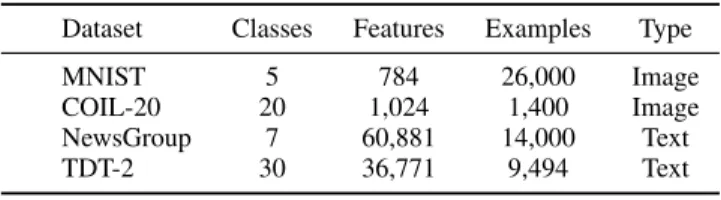
TABLE 1: Description of datasets used in experiments Dataset Classes Features Examples Type
MNIST 5 784 26,000 Image
COIL-20 20 1,024 1,400 Image NewsGroup 7 60,881 14,000 Text TDT-2 30 36,771 9,494 Text
TABLE 2: Make-up of MNIST Stream.
0 1 2 3 4 01-04k 2,000 2,000 0 0 0 05-08k 1,332 1,332 1,336 0 0 09-10k 500 500 500 500 0 11 -14k 800 800 800 800 8000 15-18k 0 1,000 1,000 1,000 1,000 19-22k 0 0 1,332 1,332 1,336 23-26k 0 0 0 2,000 2,000 the feature is SSi = N1 N P j=1
Xij2. To apply the mask, we
multiply each feature by its counterpart in the binary DFM and consider only the non-zero features.
ˆ LSi= 1 N N X j=1 Xijdf mi (11) ˆ SSi= 1 N N X j=1 Xij2df mi (12)
For the incoming pointpwe do the same: ˆ
pi =pidf mi (13)
The process of maintaining the DFM and clustering using it is outlined in Algorithm 1.
V. EXPERIMENTAL STUDY
In this section we present our experimental results using the proposed method. We describe the metrics and evaluate the method on four high-dimensional data streams, exhibiting feature drift, feature evolution, concept drift and concept evolution. We then perform a sensitivity analysis and offer some discussion on the results.
A. PERFORMANCE METRICS
Discovered clusters are evaluated across four metrics: Puri-ty, F-Measure [32], Rand Index [43] and Cluster Mapping Measure [34]. In each of the datasets we use, we know the “correct” solution as each instance is labelled. Accordingly, the clustering performance is measured with respect to this ground truth. With each metric, the ideal clustering solution will have a value close to 1 and a poor solution will have a value close to 0.
Purity measures how homogeneous a cluster is. The F-Measure (sometimes called F-Score or F1-Score) is the har-monic mean of the precision and recall scores. The Rand
Index measures the accuracy of the clustering solution. It rewards true positives and true negatives and penalises false positives and false negatives.
In the following,Rrepresents the clustering result returned by the algorithm. R containsnclusters. In every identified clusterRi(i={1,· · · , n}),Virepresents the most
frequent-ly appearing class label in clusterRi,Vsumi is the number of
instances ofViinR
i, andVtotali represents the total number
of instances of Vi in the current window. From these, we
define the following features for clusterRi: precisionRi = Vi sum |Ri| (14) recallRi = Vi sum Vi total (15) ScoreRi= 2∗ precisionRi∗recallRi precisionRi+recallRi (16) We can now express Purity (P) and F-Measure (F) in terms of the total number of clusters discovered, as follows:
P = 1 n n X i=1 precisionRi (17) F = 1 n n X i=1 ScoreRi (18)
The Rand Index (R) is a measure of agreement between two clustering solutions; the solution identified by the algo-rithm and the ground truth, which is defined as follows:
R= T P +T N
T P +F P +T N+F N, (19)
where T P, T N,F P, and F P denote the number of true positive, true negative, false positive and false negative de-cisions, respectively.
Unlike the previous three metrics, the Cluster Mapping Measure (CMM) was developed specifically for evaluating evolving data streams. The metric considers aging points, missed points, misplaced points, and noise. It is based on a mapping component which handles disappearing and emerg-ing clusters. The metric is described in detail in [34].
B. DATASETS
Here, we describe the four datasets used to evaluate our proposed method: two image-streams and two text-streams. An overview is presented in Table 1.
We first take the popular MNIST benchmark datasetand convert it to a stream in order to simulate concept and feature drift. MNIST consists of 26,000 grey scale, handwritten digits. To convert to a stream, we take five classes from the original dataset (digits 0-4) and introduce them to the stream in a sequential order. The first 4,000 instances contain images of digits 0 and 1 (shuffled), the following 4,000 points contain images of digits 0, 1 and 2, and so on. The makeup of the stream is presented in Table 2. The features in this stream are
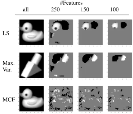
TABLE 3: Features selected on COIL-20 #Features all 250 150 100 LS Max. Var. MCFS
pixels and the discriminatory power of a pixel will change over the course of the stream.
For example, the subset of pixels which can best describe digits 0 and 1 might not be useful to discriminate between the digits which appear later in the stream.
The second image stream is the Columbia Object Image Library (COIL-20) dataset [41], which consists of 1,440 nor-malised grey scale images. Images of 20 household objects are taken at different angles. We convert it to a stream by reading the data in order. The different image classes arrive in sequence (class 1, then class 2 etc.). These different images simulate concept drift; for example, the stream might contain an image of a toy race-car, then an image of a tea-cup. The subset of features (in this case, pixels) which are useful to describe the race-car is perhaps not the best subset of pixels to describe the tea-cup. In this way feature drift is simulated. We further evaluate the proposed method on two bench-mark text-streams: 20Newsgroups and the Topic Detection and Tracking Corpus (TDT-2). 20Newsgroups is a collection of 14,000 documents separated into 7 topics and further divided into 20 different sub-topics. Some of these sub-topics are very closely related (for example, PC Hardware and Mac Hardware), so in our evaluation we take the root of the topic as the ground truth, this gives 7 topics: ‘Alternative’, ‘Com-puters’, ‘Miscellaneous’, ‘Recreation’, ‘Science’, ‘Society’, and ‘Talk’.
We split the datasets into chunks of 1,000 and shuffle each chunk in order to remove any bias (for example, a window containing only documents belonging to a single topic). We shuffle chunk-by-chunk in order to maintain the progression of topics in the stream and each chunk contains between 2 and 5 topics. As a pre-processing step we remove stop words (‘a’, ‘the’, ‘and’, etc.) from the data-set giving a feature space of 60,881 words. We refer to this data stream as Newsgroup (as opposed to 20Newsgroups). As old topics disappear from the stream and new topics are introduced, concept drift is simulated. The features (in this case, words) which are useful to describe one topic might not be useful to describe another. For example, ‘RAM’, ‘Keyboard’, ‘JPEG’ might be useful
TABLE 4: Performance of different selection methods on COIL-20 using Purity (P), F-Score (F), Rand-Index (R), and Cluster Mapping Measure (C)
#features LS MCFS Var
P F R C P F R C P F R C 250 0.86 0.69 0.73 0.89 0.94 0.87 0.86 0.96 0.86 0.77 0.75 .89 150 0.84 0.68 0.73 0.89 0.92 0.87 0.86 0.95 0.86 0.77 0.73 .90 100 0.87 0.75 0.75 0.90 0.89 0.87 0.84 0.95 0.86 0.74 0.72 .90
TABLE 5: Average clustering performance over COIL-20 Stream
Purity F-Score Rand Index CMM Dynamic Mask 0.94 0.87 0.86 0.96
Static Mask 0.91 0.74 0.79 0.93 No Mask 0.92 0.81 0.81 0.94
features to describe the concept ’computers’ but useless to describe ’Society’. In this way feature drift is simulated.
TDT-2 [21] consists of data taken from 6 sources; 2 news-wires, 2 radio, and 2 television programmes. We use TDT-2 which consists of 2 months of reports and is often used as the training set in text-classification tasks. It consists of 9,494 documents divided into 30 topics. Again, we remove stop words, divide the data-set into chunks of 1,000 and shuffle each chunk to remove any bias and simulate a stream by reading the data in sequential order.
C. EVALUATION
In this section, we evaluate clustering performance using the proposed DFM on 4 high-dimensional data streams. On each stream:
• We evaluate three different selection methods for creat-ing and maintaincreat-ing the DFM;
• We evaluate the performance of a clustering algorithm with the DFM, without a mask, and with a static mask. The static mask performs feature selection on the first window and is never updated as the stream progresses. On the COIL stream, we use aβ-window of 100 points and evaluate three unsupervised methods to maintain the mask. The first window contains two classes. We evaluate feature-subsets of different sizes (the top 250 features, the top 150, and the top 100) and we try to recreate the original images using the selected features. This is illustrated in Table 3. LS and Var appear to select similar features. The clustering performance using a DFM with different selectors and feature sizes is presented in Table 4. MCFS with 250 features creates the best DFM across the three metrics.
The comparative performance of the DFM with a static mask and no mask is presented in Table 5. Clustering using the DFM returns a better performance than clustering without a mask. Clustering using a static mask returns the worst performance out of the three.
The MNIST stream has a larger number of samples but fewer dimensions, we use a β-window of 1,000 points and evaluate three unsupervised methods to maintain the mask.
TABLE 6: Features selected on MNIST #Features all 100 50 25 LS Max. Var. MCFS
TABLE 7: Performance of different selection methods on MNIST using Purity (P), F-Score (F), Rand-Index (R), and Cluster Mapping Measure (C)
#features LS MCFS Var
P F R C P F R C P F R C 100 0.84 0.74 0.79 0.89 0.87 0.78 0.82 0.92 0.78 0.74 0.79 0.81
50 0.81 0.74 0.78 0.88 0.85 0.78 0.81 0.91 0.78 0.74 0.79 0.81 25 0.77 0.72 0.78 0.85 0.77 0.70 0.73 0.87 0.76 0.72 0.78 0.81
The first window contains two classes: digits 0 and 1. We evaluate feature-subsets of different sizes (the top 100 features, the top 50, and the top 25) and the features selected by each FS method are displayed in Table 6. As in COIL, LS and Var. appear to select similar features. The average performance using each FS method (with different feature subset sizes) over the entire stream is presented in Table 7. Again, MCFS creates a better mask than LS and Var.
We also report the time each algorithm requires in Table 8. LS and Var appear to select similar features but LS takes substantially longer. The clustering performance using a DFM with different selectors and feature sizes is presented in Table 7. MCFS with 100 features creates the best DFM across the three metrics. The comparative improvement (in three metrics and required time) in the underlying clustering algorithm (MDSC) is illustrated in Fig. 1.
The DFM improves clustering on all three metrics and also requires less time. This is because fewer pair-wise distance calculations are required. Without a mask, measurements are taken along each of the dimensions but with a mask only the important features are considered.
This time measurement includes the time it takes to per-form feature selection. The static mask is fastest; it requires fewer pairwise calculations and does not perform feature selection after the first window. Although it is faster, the performance suffers and it is better to use no mask at all rather than a static mask.
The text-streams have much higher dimensionality than the grey-scale images. So, we take larger feature subsets (up to 500 features) and we use a window-size of 1,000.
1
6
11
0
.
5
1
Time
F eature V alue`Space'
`jpeg'
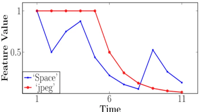
1FIGURE 2: Tracking feature-drift on two words in the NewsGroup stream.
TABLE 8: Average time required (secs.) for feature selection on different window sizes
1k 2k 5k
Var 0.01 (.005) 0.02 (001) 0.05 (.003) LS 2.71 (.01) 11.6 (.03) 76.3 (.29) MCFS 0.63 (.01) 1.34 (.006) 3.75 (.04) TABLE 9: Selection methods for creating the DFM on News-Group stream #features LS MCFS Var P F R C P F R C P F R C 500 0.93 0.74 0.64 0.94 0.91 0.65 0.48 0.91 0.90 0.77 0.76 0.91 250 0.94 0.76 0.66 0.94 0.86 0.74 0.61 0.90 0.88 0.79 0.78 0.91 150 0.94 0.76 0.67 0.95 0.87 0.75 0.65 0.90 0.93 0.82 0.81 0.93
TABLE 10: Average clustering performance over News-Group Stream
Purity F-Score Rand Index CMM Dynamic Mask 0.93 0.82 0.81 0.93
Static Mask 0.85 0.76 0.72 87
No Mask 0 0 0 0
Over the entire stream, the Maximum Variance selection method creates the best mask as can be seen in Table 9. The first window contains two topics: ‘Alternative’ and ‘Com-puters’. The top 5 features selected by Maximum Variance are: {jpeg, image, graphics, Jesus, God}. Using the Feature Values vector, which is updated after each window, we can track the importance of a word as it changes over time. As an illustrative example, we take two words selected in the first window - ‘jpeg’ and ‘space’. Their perceived importance over the course of the stream is displayed in Fig. 2. ‘jpeg’ is considered important for the first five windows but begins to lose importance as the ‘computers’ topic disappears from the stream. It is never selected again and by the end of the stream its perceived importance is zero. ‘Space’ is also selected in the context of computing and its importance drops as the ‘computing’ topic disappears from the stream. However, the word becomes relevant again later in the stream, in a different
1
5
10
15
20
25
0
.
4
1
Purit yNo Mask
Dynamic Mask
Static Mask
11
5
10
15
20
25
0
.
4
1
F-ScoreNo Mask
Dynamic Mask
Static Mask
1 1 5 10 15 20 25 0.4 1 Time Rand-Index Dynamic MaskNo MaskStatic Mask 1 1 5 10 15 20 25 0 1 2.2 Time Secconds
No Mask Dynamic Mask Static Mask
1
FIGURE 1: Comparative improvement in clustering performance on the MNIST stream
context; ’space’ is once again selected when the ‘Science’ topic is present in the stream. ‘Space’ is selected along side features such as ‘satellite’, ‘NASA’, and so on.
The performance of the clustering algorithm (with the DFM) over the course of the stream is presented in Table. 10. Without a mask, no clustering solution is found. This is likely because of the high dimensionality (>60,000). However, with a static mask of 150 features, a solution is returned. Clustering performance is further improved using a dynamic mask.
On the TDT-2 stream, the Maximum Variance selection method provides the best DFM. The comparative perfor-mance with the other two selection methods is displayed in Table 11, and the clustering improvement in Table 12.
The results across each data stream are summarised in Table 13. On each of the four data streams, on all three metrics, the MDSC algorithm is improved using the proposed DFM.
In all of the previous experiments described we used MDSC to test the proposed DFM. We also evaluate on three other density based cluster algorithms; Ant Colony Stream Clustering (ACSC) [19], CEDAS [31], and DenStream [14]. On each dataset, we use the best selection method discovered in previous experiments; MCFS with 100 and 250 features for MNIST and COIL, respectively, and Maximum Vari-ance with 150 and 250 features for Newsgroup and TDT-2, respectively. The comparative results are displayed in Table 14 using ACSC, Table 15 using CEDAS, and Table 16 for DenStream. On every stream, each of the underlying clustering algorithms is improved by the proposed DFM.
TABLE 11: Performance of different selection methods for creating the DFM on TDT-2 stream
#features LS MCFS Var
P F R C P F R C P F R C 500 0.77 0.60 0.61 0.82 0.80 0.62 0.61 0.83 0.72 0.63 0.62 0.80 250 0.77 0.60 0.58 0.82 0.79 0.63 0.62 0.84 0.83 0.63 0.88 0.87 150 0.81 0.59 0.58 0.84 0.77 0.62 0.61 0.84 0.83 0.62 0.58 0.88
TABLE 12: Clustering performance over TDT-2 Stream Purity F-Score Rand Index CMM Dynamic Mask 0.83 0.62 0.61 0.87
Static Mask 0.72 0.61 0.60 0.80
No Mask 0 0 0 0
D. SENSITIVITY ANALYSIS
In this section, we examine the sensitivity and effect of the two parameters required to create and maintain the DFM; the threshold valueλand the window sizeβ. We experiment on the MNIST data stream described in Section V-B using MCFS with 100 features as the selector. For illustrative clarity, we use a metric ‘Score’. Score is the average of purity, Rand Index and F-Score.
λdetermines the length of time a feature remains relevant if it is no longer selected in topnfeatures. It is a threshold for the Feature Values and determines which features are considered in the clustering process. We experiment with values in the range 0.1 to 1.0. The results are displayed in Fig. 3.
Clustering performance is stable with a slight drop after a value of 0.5. If the threshold is too high (1.0 in this example), the performance suffers dramatically.
If the threshold is too high, no features are considered so
TABLE 13: Performance of Dynamic Mask with MDSC
Data Stream No Mask Static Mask Dynamic Mask
P F R C P F R C P F R C
MNIST 0.86 0.69 0.75 0.90 0.73 0.66 0.73 0.87 0.87 0.78 0.82 0.92
COIL 0.92 0.81 0.81 0.93 0.91 0.74 0.79 0.94 0.94 0.87 0.86 0.96
NewsGroup 0 0 0 0 0.85 0.76 0.72 0.87 0.93 0.82 0.81 0.93
TDT-2 0 0 0 0 0.72 0.61 0.60 0.80 0.83 0.62 0.61 0.87
TABLE 14: Performance of Dynamic Mask with ACSC
Data Stream No Mask Static Mask Dynamic Mask
P F R C P F R C P F R C
MNIST 0.89 0.69 0.75 0.94 0.75 0.65 0.73 0.88 0.92 0.80 0.84 0.94
COIL 0.86 0.79 0.74 0.93 0.85 0.74 0.72 0.86 0.92 0.82 0.79 0.93
NewsGroup 0 0 0 0 0.81 0.70 0.72 0.85 0.90 0.82 0.81 0.93
TDT-2 0 0 0 0 0.72 0.61 0.60 0.81 0.87 0.60 0.61 0.87
TABLE 15: Performance of Dynamic Mask with CEDAS
Data Stream No Mask Static Mask Dynamic Mask
P F R C P F R C P F R C
MNIST 0 0 0 0 0.78 0.62 0.61 0.83 0.91 0.64 0.73 0.91
COIL 0.5 0.17 0.53 0.62 0.99 0.67 0.72 1.00 0.99 0.69 0.75 1.00
NewsGroup 0 0 0 0 0.84 0.65 0.68 0.92 0.90 0.74 0.78 0.93
TDT-2 0 0 0 0 0.74 0.58 0.57 0.74 0.89 0.58 0.59 0.92
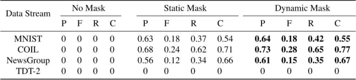
TABLE 16: Performance of Dynamic Mask with DenStream
Data Stream No Mask Static Mask Dynamic Mask
P F R C P F R C P F R C
MNIST 0 0 0 0 0.63 0.18 0.37 0.54 0.64 0.18 0.42 0.55
COIL 0 0 0 0 0.68 0.24 0.62 0.71 0.73 0.28 0.65 0.77
NewsGroup 0 0 0 0 0.56 0.12 0.34 0.66 0.61 0.15 0.35 0.67
TDT-2 0 0 0 0 0 0 0 0 0 0 0 0
the clustering process does not happen. In this case, cluster-ing would only occur on features which have been selected in every window. This is perhaps unlikely in a dynamic stream. This is illustrated in Fig. 3. Here, we display the number of features that are considered in the clustering process. We are selecting the top 100 features in each window and with a low threshold, previously important features remain relevant for a long time even if they are no longer being selected. This can be seen with a λ value of 0.01, approximately 300 features are considered as ‘important’ at each time-step. With a high threshold of 1.0, no features are considered important by the end of the stream. Using a value of 0.5, the number of selected features remains at roughly 100. For each experiment described in this paper, we use aλvalue of 0.5.
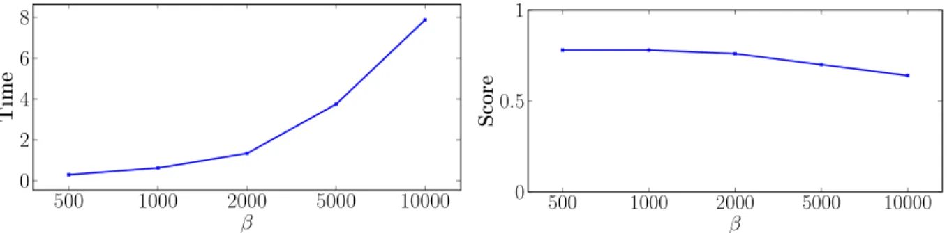
The parameterβ determines the number of points which should be collected in the buffer before feature selection
is performed and the DFM is updated. We first measure the time it takes to perform FS on different β-windows. We examine window-sizes from 500 to 10,000 and measure using seconds. The results are displayed in Fig. 4. It can be seen that the relationship between time and β is not quite linear and it is more efficient to use smaller values forβ. This is confirmed when we measure the clustering performance using the different window sizes. The score decreases as β
increases. We used a value of 1,000 forβin all experiments described except for COIL-20 which is comparatively small so we used a value of 100.
E. DISCUSSION
In each of the experiments, the proposed DFM method im-proves the performance of an underlying clustering algorith-m. This is true for each of the evaluated clustering algorithms.
.01 0.1 0.25 0.5 0.75 1.0 0.5 1 λ Score 1 1 5 10 15 20 25 0 100 200 300 Time # Feature s .01 0.1 0.25 0.5 0.75 1.0 1
FIGURE 3: Sensitivity ofλwith respect to clustering performance (left) and the effect of the parameter on the number of features considered in the clustering process (right).
500 1000 2000 5000 10000 0 2 4 6 8 β Time 1 500 1000 2000 5000 10000 0 0.5 1 β Score 1
FIGURE 4: Time required to perform FS on different values forβ(left) and sensitivity ofβwith respect to clustering performance (right).
Of the three feature selectors evaluated to create the mask, MCFS and Maximum Variance outperform the Laplacian Score. On the image streams with a lower dimensionality, the MCFS method creates the best mask. On the text-streams with higher dimensionality, Maximum Variance creates the best mask.
On the text-streams with high dimensionality (up to 60,000 features), the underlying clustering algorithms were unable to return a solution without a mask. With a static mask (a mask with features selected from the first window and never updated as the stream progresses), the performance is improved and a solution is returned.
However, a dynamic mask further improves this perfor-mance. A dynamic mask also allows the importance of a fea-ture to be observed and tracked over time. This was illustrated in the Newsgroup data stream (Fig. 2); two features were selected and their perceived importance over the course of the stream was tracked revealing feature drift. On the image-streams with a lower dimensionality, a clustering solution can be found without a mask but performance is improved with a dynamic mask. Not only is performance improved but less processing time is required. Fewer features are considered in the clustering process, therefore fewer pairwise calculations are required. On the image-streams (≈1,000 dimensions), a static mask actually deteriorates the clustering performance. This suggests that, in the presence of feature drift and concept evolution, it is preferable not to perform feature selection at all, rather than traditional static selection methods. In the presence of feature drift, as features become redundant
and new features become relevant, the static mask is never updated and clustering is performed along irrelevant features and omits newly important features.
Despite never selecting features which create the best mask, the Lapacian Score method requires the most time. On the higher dimensional text-streams, the Maximum Variance method selects the best features and also requires the least amount of time, demonstrated in Table 8. This method re-quiresO(N +d)time, whereN is the number of instances with d dimensions. MCFS takes longer time (it requires
O(N2 +d3)[13]) and was found to be better suited to the (comparatively) lower dimensional streams.
VI. CONCLUSIONS
This paper presents a Dynamic Feature Mask (DFM) for unsupervised dynamic feature selection in non-stationary data streams. Redundant features are masked and clustering is performed along unmasked, relevant features. If a feature’s perceived importance changes, the mask is updated accord-ingly - previously unimportant features can be unmasked and features which lose relevance become masked. The method is proposed to address two challenges in data stream clustering: 1) feature drift - a change at the feature level in a stream, and 2) the problem of clustering high-dimensional streams where the curse of dimensionality renders distance measurements and the concepts of ‘density’ difficult.
The proposed method is algorithm-independent and can be used with any existing density based clustering algorithm. There are many density-based clustering algorithms in the
literature and they typically do not have a mechanism to deal with feature drift or with very high-dimensionality.
We evaluated the proposed method on four density based clustering algorithms (MDSC, CEDAS,ACSC, and Den-Stream) across four high-dimensional streams; two text streams and two image streams. In each case, the proposed DFM improves clustering performance and furthermore, re-duces the processing time required by the underlying algo-rithm.
An unsupervised feature selection method is required to create and maintain the DFM and we evaluate three existing methods: Laplacian Score, Multi-Cluster Feature Selection, and Maximum Variance. Experimental results suggest that on the lower dimensional (≈1,000dimensions) streams, MCFS is the best selector for the mask. On the higher dimensional text streams (up to 60,000 dimensions), the Maximum Vari-ance method selects the best features to maintain the mask. The Laplacian Score did not return the best features on any stream and was shown to require considerably more time than the other two methods.
On each stream, we compare the DFM with a static feature mask. In the static case, the mask is created on one window at the beginning of the stream and is never updated. The dynamic mask performs better on each stream. On the higher dimensional streams, the static mask is preferable to no mask (without a mask the clustering algorithms could not return a solution at all) but on the lower dimensional streams it is preferable to use no mask rather than a static mask.
Future work will investigate the suitability of the proposed method for density-based classification methods in high-dimensional data streams with feature drift.
REFERENCES
[1] C. C. Aggarwal, J. Han, J. Wang, and P. S. Yu, “A framework for clustering evolving data streams”, Proc. 29th Int. Conf. Very Large Data Bases, vol. 29, pp. 81-92, 2003.
[2] S. Alelyani, J. Tang, and H. Liu, “Feature Selection for Clustering: A Review”, Data Clustering: Algorithms and Applications, 29, pp. 110-121, 2013.
[3] A. Amini, et al. “On density-based data streams clustering algorithms: A survey”, Journal of Computer Science and Technology, vol. 29, no. 1, pp. 116-141, 2014.
[4] J. P. Barddal, H. M. Gomes, F. Enembreck, and B. Pfahringer,“A survey on feature drift adaptation: Definition, benchmark, challenges and future directions”, Journal of Systems and Software, 127, pp.278-294. 2017. [5] J. P. Barddal, F. Enembreck, H. M. Gomes, A. Bifet, and B. Pfahringer,
“Merit-guided dynamic feature selection filter for data streams”, Expert Systems with Appl., vol. 116, pp.227-242, 2019.
[6] J. P. Barddal, F. Enembreck, H. M. Gomes, A. Bifet and B. Pfahringer, ”Boosting decision stumps for dynamic feature selection on data streams”. Inform. Syst., vol. 83, pp. 13-29. 2019.
[7] J. P. Barddal, H. M. Gomes, F. Enembreck, B. Pfahringer and A. Bifet, “On dynamic feature weighting for feature drifting data streams”. In: Joint European Conf on Machine Learning and Knowledge Discovery in Databases, pp. 129-144, 2016.
[8] J. P. Barddal, H. M. Gomes, F. Enembreck and J.P. Barthôls. “SNC-Stream+: Extending a high quality true anytime data stream clustering algorithm”. Information Systems, vol. 62, pp. 60-73. 2016.
[9] Belkin, M. and Niyogi, P., “Laplacian eigenmaps and spectral techniques for embedding and clustering”, In: Advances in neural information pro-cessing systems, pp. 585-591, 2002.
[10] V. Bhatnagar,S. Kaur, and S. Chakravarthy, “Clustering data streams using grid-based synopsis”, Knowledge and Information Systems, vol. 41, no. 1, pp. 127-152, 2014.
[11] J. Biesiada and W. Duch, “Feature selection for high-dimensional data; a Pearson redundancy based filter”, In: Computer Recognition Systems 2, Springer, Berlin, Heidelberg, pp. 242-249, 2007.
[12] A. Bifet and R. GavaldÃ˘a, “Adaptive learning from evolving data stream-s”. In: International Symposium on Intelligent Data Analysis, pp. 249-260, 2009.
[13] D. Cai, C. Zhang, and X. He, “Unsupervised feature selection for multi-cluster data”, In: Proc. 16th ACM SIGKDD Int. Conf. on Knowledge Discovery and Data Mining, pp. 333-342, 2010.
[14] F. Cao, M. Ester, W. Qian, and A. Zhou, “Density-based clustering over an evolving data stream with noise”, SDM, vol. 6, pp. 328–339, 2006. [15] V.R. Carvalho and W.W. Cohen, “Single-pass online learning:
Perfor-mance, voting schemes and online feature selection”, In: Proc. 12th ACM SIGKDD Int. Conf. Knowledge Discovery and Data Mining, pp. 548-553, 2009.
[16] G. Chandrashekar and F. Sahin, “A survey on feature selection methods”, Computers & Electrical Engineering, vol. 40, no. 1, pp. 16-28, 2014. [17] M. Ester, H.P Kriegel, J. Sander, and X. Xu, “A density-based algorithm
for discovering clusters in large spatial databases with noise”, In KDD, Vol. 96, No. 34, pp. 226-231, August, 1996.
[18] A. H. Fahim, A. M. Salem, F. A. Torkey, and M. A. Ramadan, “Density Clustering Based on Radius of Data (DCBRD)”, World Academy of Science, Engineering and Technology, 2006.
[19] C. Fahy, S. Yang and M. Gongora, “Ant colony stream clustering: A fast density clustering algorithm for dynamic data streams”, IEEE Trans. Cybern., vol. 49, no. 6, pp. 2215-2228, June 2019.
[20] C. Fahy and S. Yang, “Finding and tracking multi-density clusters in an online dynamic data stream”, IEEE Trans. Big Data, in press, 2019. [21] J. Fiscus, G. Doddington, J. Garofolo and A. Martin, “NISTâ ˘A ´Zs 1998
Topic Detection and Tracking evaluation (TDT2)”, In: Proc. 1999 DARPA Broadcast News Workshop pp. 19-24, 1999.
[22] A. Forestiero, C. Pizzuti, and G. Spezzano, “A single pass algorithm for clustering evolving data streams based on swarm intelligence”, Data Mining and Knowledge Discovery, vol. 26, no. 1, pp. 1-26, Nov. 2011. [23] Y. Freund, R. Schapire, and N. Abe, “A short introduction to
boost-ing”. Journal-Japanese Society For Artificial Intelligence, 14(771-780), pp. 1612, 1999.
[24] H. M. Gomes, A. Bifet, J. Read, J.P. Barddal, F. Enembreck, B. Pfharinger, G. Holmes, and T. Abdessalem. “Adaptive random forests for evolving data stream classification”. Machine Learning, vol. 106, no. 9-10, pp.1469-1495, 2017.
[25] Q. Gu, Z. Li, and J. Han, “Generalized Fisher score for feature selection”, In: Proc. 27th Int. Conf. on Uncertainty in Artif. Intell. (UAI’11), pp. 266-273, 2011.
[26] S. Guha, and N. Mishra. “Clustering data streams”, Data Stream Manage-ment. Springer Berlin Heidelberg, pp. 169-187, 2016.
[27] M. Hall, “Correlation-based feature selection for machine learning”, PhD Thesis, Department of Computer Science, Waikato University, New Zealand, 1999.
[28] X. He, D. Cai, and P. Niyogi, “Laplacian score for feature selection”, In: Advances in Neural Information Processing Systems, pp. 507-514, 2006. [29] C. L. Huang,and C.J. Wang, “A GA-based feature selection and parameters
optimization for support vector machines”, Expert Systems with applica-tions, vol. 31, no. 2, pp. 231-240, 2006.
[30] H. Huang, S. Yoo, and S.P. Kasiviswanathan, “Unsupervised feature selection on data streams”, In Proceedings of the 24th ACM International on Conference on Information and Knowledge Management, pp. 1031-1040, October 2015.
[31] R. Hyde, P. Angelov, and A. R. MacKenzie, “Fully online clustering of evolving data streams into arbitrarily shaped clusters”, Information Sciences, vol. 382-383, pp. 96–114, 2017.
[32] N. Jardine and C. J. van Rijsbergen, “The use of hierarchic clustering in information retrieval”, Information Storage and Retrieval, vol. 7, no. 5, pp. 217–240, Dec. 1971.
[33] I. Katakis, G. Tsoumakas, and I. Vlahavas, “On the utility of incremental feature selection for the classification of textual data streams”, In: Panhel-lenic Conference on Informatics, pp. 338-348, November 2005. [34] H. Kremer, P. Kranen, T. Jansen, T. Seidl, A. Bifet, G. Holmes, and B.
Pfahringer “An effective evaluation measure for clustering on evolving data streams”. In: Proc. 17th ACM SIGKDD Int. Conf. on Knowledge Discovery and Data Mining, pp. 868-876, 2011.
[35] M.H. Law, M.A Figueiredo, and A,K Jain, “Simultaneous feature selection and clustering using mixture models”, IEEE Transactions on Pattern Analysis and Machine Intelligence, vol. 26, no. 9, pp. 1154-1166. 2004 [36] C. Lee and G. G. Lee, “Information gain and divergence-based feature
selection for machine learning-based text categorization”, Information Processing & Management, vol. 42, no. 1, pp. 155-165, 2006.
[37] J. Li et al., “Feature selection: A data perspective”, ACM Computing Surveys, vol. 50, no. 6, pp.94, 2017.
[38] Z. Ma, H. Yu, W. Chen, and J. Guo. “Short utterance based speech lan-guage identification in intelligent vehicles with time-scale modifications and deep bottleneck features”. IEEE Trans. Vehicular Tech., vol. 68, no. 1, pp.121-128. 2018
[39] Z. Ma, Y. Lai, W.B. Kleijn, Y.Z. Song, L. Wang, and J. Guo, J. “Variational Bayesian learning for Dirichlet process mixture of inverted Dirichlet dis-tributions in non-Gaussian image feature modeling”, IEEE Trans. Neural Networks and Learning Systems, (99), pp.1-15. 2018.
[40] M. Masud, J. Gao, L. Khan, J. Han and B.M. Thuraisingham, “Classifica-tion and novel class detec“Classifica-tion in concept-drifting data streams under time constraints”, IEEE Trans. Knowledge and Data Engineering, vol. 23, no. 6, pp.859-874, 2011.
[41] S. A. Nene, S. K. Nayar, and H. Murase, ”Columbia object image library (coil-20)”, Technical Report, Columbia University, 1996.
[42] H.L Nguyen, Y.K. Woon, W.K. Ng and L. Wan, “Heterogeneous ensemble for feature drifts in data streams”, In Pacific-Asia Conference on Knowl-edge Discovery and Data Mining, Springer, Berlin, Heidelberg. pp. 1-12, May 2012.
[43] W. M. Rand, “Objective criteria for the evaluation of clustering methods”, Journal of the American Statistical Assoc., vol. 66, no. 336, pp. 846, Dec. 1971.
[44] G. Roffo, S. Melzi and M. Cristani, “Infinite feature selection”, In: Pro-ceedings of the 2015 IEEE Int. Conf. on Computer Vision, pp. 4202-4210, 2015.
[45] L. Tu and Y. Chen, “Stream data clustering based on grid density and attraction”, ACM Trans. Knowledge Discovery from Data, vol. 3, no. 3, Article 12, 27 pages, July 2009.
[46] L. Wang, and H. Shen, “Improved Data Streams Classification with Fast Unsupervised Feature Selection”, In: Proceedings of the 17th IEEE Int. Conf. on Parallel and Distributed Computing, Applications and Technolo-gies (PDCAT), pp. 221-226, December 2016.
[47] L. Wan, W. K. Ng, X. H. Dang, P. S. Yu, and K. Zhang, “Density-based clustering of data streams at multiple resolutions”, ACM Trans. Knowledge Discovery from Data, vol. 3, no. 3, Article 14, 28 pages, July 2009.
[48] F. Wilcoxon,and R. A. Wilcox. “Some rapid approximate statistical proce-dures”, Lederle Laboratories, 1964.
[49] H. Yu, Z.H. Tan, Z. Ma, R. Martin, and J. Guo, “Spoofing detection in automatic speaker verification systems using DNN classifiers and dynamic acoustic features”. IEEE Trans. Neural Networks and Learning Systems, vol. 29, no. 10, pp. 4633–4644, Oct. 2018.
CONOR FAHYreceived the BSc degree in Com-puter Science from Dublin City University, Ire-land in 2004. He received the MSc degree in Intelligent Systems and PhD degree in Computer Science from De Montfort University, Leicester, UK in 2016 and 2019, respectively. Since June 2019, he has been a Lecturer within the School of Computer Science and Informatics, De Montfort University, Leicester, UK. His research interests include swarm intelligence and ensemble methods for unsupervised and semi-supervised learning in dynamic environments.
SHENGXIANG YANG(M’00–SM’14) received the B.Sc. and M.Sc. degrees in automatic con-trol and the Ph.D. degree in systems engineering from Northeastern University, Shenyang, China in 1993, 1996, and 1999, respectively.
He is currently a Professor in Computational Intelligence and Director of the Centre for Compu-tational Intelligence, School of Computer Science and Informatics, De Montfort University, Leices-ter, U.K. He has over 280 publications. His current research interests include evolutionary computation, swarm intelligence, artificial neural networks, data mining and data stream analysis, and relevant real-world applications. He serves as an Associate Editor/Editorial Board Member of several international journals, such as the IEEE Transactions on Cybernetics, IEEE Transactions on Evolutionary Computation, Information Sciences, Enterprise Information Systems, and Soft Computing.