Scholarship@Western
Scholarship@Western
Electronic Thesis and Dissertation Repository
3-26-2020 10:00 AM
Hyperspectral Image Classification for Remote Sensing
Hyperspectral Image Classification for Remote Sensing
Hadis Madani
The University of Western Ontario
Supervisor
McIsaac, Kenneth
The University of Western Ontario
Graduate Program in Electrical and Computer Engineering
A thesis submitted in partial fulfillment of the requirements for the degree in Doctor of Philosophy
© Hadis Madani 2020
Follow this and additional works at: https://ir.lib.uwo.ca/etd
Part of the Other Electrical and Computer Engineering Commons
Recommended Citation Recommended Citation
Madani, Hadis, "Hyperspectral Image Classification for Remote Sensing" (2020). Electronic Thesis and Dissertation Repository. 6940.
https://ir.lib.uwo.ca/etd/6940
This Dissertation/Thesis is brought to you for free and open access by Scholarship@Western. It has been accepted for inclusion in Electronic Thesis and Dissertation Repository by an authorized administrator of
This thesis is focused on deep learning-based, pixel-wise classification of hyperspectral images (HSI) in the field of remote sensing. Although presence of many spectral bands in an HSI provides a valuable source of features which favors classification methods, dimen-sionality reduction is often performed in the pre-processing step to reduce the correlation between bands and spectral dimension of the input HSI. Most of the deep learning-based classification algorithms use unsupervised dimensionality reduction methods such as prin-cipal component analysis (PCA) which does not consider class labels. In this thesis, in order to take advantage of class discriminatory information in the dimensionality reduc-tion step as well as the power of deep neural network in extracting abstract, deep features of HSI datasets, we propose a new method that combines a supervised dimensionality reduction technique, principal component discriminant analysis (PCDA) and deep learn-ing. One common problem in remote sensing HSI classification is the lack of enough reliable ground truth samples. One solution to this dilemma can be data augmentation where virtual samples are generated from the ground truth examples. In this thesis, we propose a simple spectral perturbation method to augment the number of available training samples and improve the classification results.
Since combining spatial and spectral information for classifying hyperspectral images can dramatically improve the performance, in this thesis we also propose a new spectral-spatial feature vector. In our feature vector, based on their proximity to the dominant edges in the HSI, neighbors of a target pixel have different contributions in forming the spatial information. To obtain such a proximity measure, we propose a method to compute the distance transform image of the input HSI. We then improved the spatial feature vector by adding extended multi attribute profile (EMAP) features to it. Clas-sification accuracies demonstrate the effectiveness of our proposed method in generating a powerful, expressive spectral-spatial feature vector.
Keywords: Remote sensing, hyperspectral image (HSI) classification, machine
learn-ing, stacked autoencoder (SAE), deep learnlearn-ing, supervised dimensionality reduction,
profile (EMAP), neural network (NN).
In this thesis, we propose a few approaches to perform hyperspectral image (HSI) clas-sification in the field of remote sensing. As opposed to the regular RGB images which consist of three channels of red, green, and blue, an HSI is composed of a series of images each taken at a specific wavelength. In the field of remote sensing, hyperspectral images are collected by the imaging sensors on board of an airplane or a satellite and due to the valuable information that they can provide about the objects and phenomena on our planet, they are employed in many applications.
One common practice in HSI processing is the classification of each individual pixel in the image. In other words, in many applications we are interested in assigning each pixel to a specific category. This kind of classification has been an active research area for years for which different approaches have been proposed. Recently, deep learning-based methods have attracted a lot of attention from the research community because of their superior performance compared to the conventional methods. Therefore, in this thesis, we used one of the deep learning frameworks, stacked autoencoder (SAE) to perform the pixel-wise HSI classification task.
As our first contribution, we combined SAE with a supervised dimensionality reduc-tion (DR) technique where labels of the samples are used during the DR step. Second, as one of the common issues in processing the remote sensing hyperspectral datasets is the lack of enough labeled data, we proposed a method to generate virtual samples using the available ground truth data. Since combining spectral and spatial information in an HSI, can dramatically improve classification accuracies as our third contribution, in this thesis project we proposed a new method including a novel spectral-spatial feature vector. In our spatial feature vector, effective pixels have different contributions based on an edge proximity measure obtained from the distance transform image of the input HSI. We ap-plied our methods on several remote sensing hyperspectral datasets and evaluated their performance using various accuracy metrics. Classification results show the superiority of our methods compared to several conventional and deep learning-based approaches.
To my parents,
and my husband,
for their endless love and generous support.
I would like to express my sincere gratitude to Dr. Kennth McIsaac for his excellent su-pervision, immense knowledge, and continuous encouragement throughout the course of this research. It has been a great privilege and honor to pursue my higher education under his supervision.
I would like also to acknowledge Prof. J. Wang and Dr. B. Feng for providing us the Surrey dataset along with the ground truth image.
Thanks as well to the team members of the research group for their kindness, valuable feedback and helpful discussions.
Abstract i
Summary for Lay Audience iii
Dedication iii
Acknowledgments v
List of Figures ix
List of Tables xiii
List of Acronyms xv
1 Introduction 1
1.1 Remote sensing . . . 1
1.1.1 Definition and applications . . . 1
1.1.2 Remote sensing mission examples . . . 4
1.2 Research problem . . . 6
1.2.1 Hyperspectral image classification . . . 6
1.3 Research contributions . . . 8
2 Background and Literature Review 9 2.1 Background . . . 9
2.2 Literature review . . . 12
2.3 Machine learning and image processing . . . 18
2.3.1 Principal Component Analysis . . . 19
2.3.2 Linear Discriminant Analysis (LDA) . . . 22
2.3.3 Artificial neural networks (ANN) . . . 27
2.3.3.1 Single layer neural network (perceptron) . . . 28
2.3.3.2 Multi layer neural network . . . 30
2.3.4 Deep neural network . . . 33
2.3.4.1 Stacked autoencoder . . . 33
2.3.4.2 Sparse autoencoder . . . 35
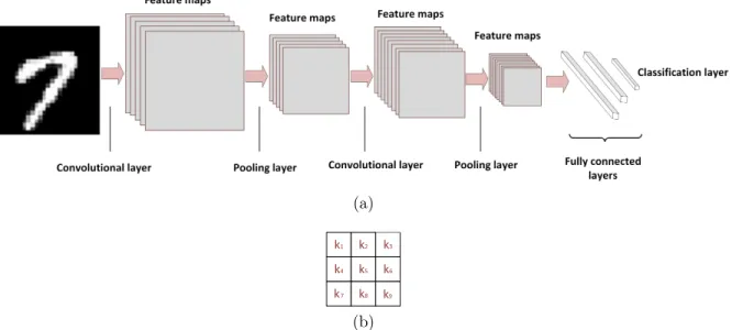
2.3.4.3 Convolutional neural network . . . 37
2.3.4.4 Deep belief network . . . 38
2.3.4.5 Recurrent neural network . . . 40
2.3.5 Extended multi-attribute profile . . . 42
2.3.5.1 Morphological profiles . . . 42
2.3.5.2 Extended morphological profiles (EMP) . . . 43
2.3.5.3 Attribute profiles . . . 44
2.3.5.4 Max-Tree . . . 46
2.3.5.5 Extended attribute profiles . . . 48
2.4 Summary . . . 51
3 Hyperspectral Image Classification Using PCDA and SAE 52 3.1 Introduction . . . 52
3.2 Method . . . 55
3.2.1 Proposed framework . . . 55
3.2.2 Principal component discriminant analysis . . . 56
3.3 Experimental results . . . 58
3.3.1 Data description . . . 58
3.3.2 Parameter tuning . . . 61
3.3.3 Performance evaluation . . . 65
3.4 Conclusion . . . 71
4 Distance transform based spectral-spatial feature vector for HSI classifica-tion with SAE 74 4.1 Introduction . . . 74
4.3.1 HYPERSPECTRAL DATASETS . . . 82
4.3.1.1 Salinas . . . 82
4.3.1.2 University of Pavia . . . 82
4.3.1.3 Surrey . . . 82
4.3.2 Parameter Tuning . . . 84
4.3.2.1 Number of retained PCs and size of the neighborhood . . . 85
4.3.2.2 Size of the hidden layers . . . 88
4.3.2.3 Required threshold parameters . . . 88
4.3.3 Performance Evaluation . . . 89
4.3.3.1 Effect of using supervised dimensionality reduction . . . 89
4.3.3.2 Comparison with other methods . . . 91
4.4 Conclusion . . . 94
5 Spectral perturbation method for deep learning-based classification of re-mote sensing hyperspectral images 99 5.1 Introduction . . . 99 5.2 Method . . . 100 5.3 Experimental Results . . . 102 5.3.1 Data Description . . . 103 5.3.2 Performance Evaluation . . . 104 5.4 Conclusion . . . 109 6 Conclusion 110 Bibliography 114 Curriculum Vitae 123 viii
1.1 Two main types of remote sensing. (a) Airborne and (b) space-borne remote sensing. . . 2 1.2 Active versus passive remote sensor. In passive remote sensing, Sun is often the
source of energy whereas in active remote sensing, the airplane/satellite carries the energy source. . . 3 1.3 A sample hyperspectral image. This hyperspectral database was taken with
Reflective Optics System Imaging Spectrometer (ROSIS) during a flight over Pavia University, in northern Italy. . . 7
2.1 Electromagnetic spectrum . . . 10 2.2 Concept of hyperspectral imaging. A large area on the ground is being imaged by
an airborne/spaceborne imaging device covering a wide range of electromagnetic spectrum. Different reflectance values for the three sample materials in the scene depicts how different classes can be identified using their reflectance values. . . 11 2.3 A toy example showing the directions of maximum variance in the data obtained
by the PCA algorithm . . . 19 2.4 A toy example showing the best projection directions suggested by PCA and
LDA algorithms. . . 23 2.5 Graphical representation of a single layer NN with only one hidden neuron which
functions similar to a perceptron. . . 29 2.6 Several activation functions. (a) Sigmoid, (b) tanh, (c) ReLU. . . 29 2.7 Schematic of a sample multilayer neural network with input data with three
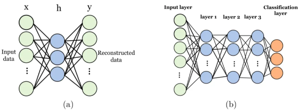
features, one hidden layer with four hidden units, and the output layer with three nodes corresponding to a three-class classification problem. . . 31 2.8 Block diagram of (a) a sample auto-encoder and (b) stacked autoencoder . . . . 33
2.10 A sample RBM. . . 39 2.11 (a) Schematic of an RNN (b) unfolded network shown in (a). . . 40 2.12 RNN (a) One to many and (b) many to one architectures. . . 41 2.13 Max -tree representation. (a) a synthetic gray-scale image and (b) max-tree
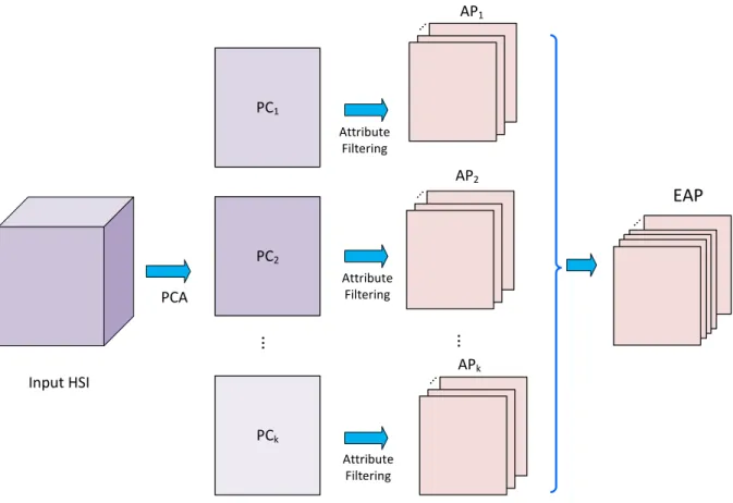
structure of image in (a). . . 47 2.14 Process of obtaining the extended attribute profile from an HSI input where k
principal components are preserved in the PCA dimensionality reduction step. . 49 2.15 Schematic of the step by step process of building the EMAP structure by keeping
the first k PCs and using n attribute filters. . . 50
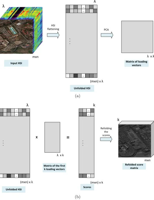
3.1 Steps of applying PCA on an HSI. (a) Unfolding the input HSI and computing the λ eigenvectors (loading vectors). (b) Multiplying the unfolded HSI by the first k loading vectors and folding the result back in the form of a cube. . . 53 3.2 Block diagram of the proposed method. PCDA is employed to capture spatial
information of each target pixel which then will be stacked with the spectrum of the target pixel to form the input of the SAE network. This network is composed of multiple sparse autoencoders. . . 56 3.3 Indian Pines dataset. (a) False color image and (b) pseudo ground truth image. 59 3.4 University of Pavia dataset. (a) True color image and (b) pseudo ground truth
image. . . 60 3.5 Distribution of the OA obtained by our method with different values for then1
andn2 for Indian Pines dataset using neighborhood sizes of (a)3×3, (b)5×5, and (c)7×7. . . 63 3.6 Distribution of the OA obtained by our method with different values for then1
andn2 for University of Pavia dataset using neighborhood sizes of (a)3×3, (b) 5×5, and (c)7×7. . . 64 3.7 Distribution of the OA obtained by our method using different values for then1
and n2 for (a) Indian Pines and (b) University of Pavia datasets. . . 65 3.8 Distribution of the OA of our method vs different values of the number of hidden
units for (a) Indian Pines and (b) University of Pavia datasets. . . 66
3.10 Distribution of the OA obtained by DAE-LR using different values for n1 and the neighborhood size for the University of Pavia dataset. . . 67 3.11 Indian Pines.(a) Ground truth and classification maps obtained from different
methods using 20% of labeled data for training. (b)RBF-SVM, (c) PCDA-SVM, (d) DAE-LR, (e) EMAP-PCDA-SVM, (f) CNN-PPF-LR, (g) EMAP-SAE, and (h) PCDA-SAE. . . 72 3.12 University of Pavia.(a) Ground truth and classification maps obtained from
dif-ferent methods using 10% of labeled data for training. (b)RBF-SVM, (c) PCDA-SVM, (d) DAE-LR, (e) EMAP-PCDA-SVM, (f) CNN-PPF-LR, (g) EMAP-SAE, and (h) PCDA-SAE. . . 73
4.1 Schematic of the justification of using the distance transform in the spatial feature vector. . . 76 4.2 Steps of obtaining the distance transform image of the Salinas hyperspectral
dataset. . . 78 4.3 Block diagram of our proposed method. The cube shown in the top row depicts
only a neighborhood region around the blue pixel. Also, the spectral dimen-sionality of the input HSI (not shown in this figure) is reduced using the PCA method and as an example 3 PCs are retained. . . 79 4.4 Block diagram of the proposed feature vector obtained by PCDA and distance
transform values. . . 81 4.5 Salinas dataset. (a) False color image. (b) Pseudo ground truth image. . . 83 4.6 University of Pavia dataset. (a) True color image. (b) Pseudo ground truth
image. . . 85 4.7 Surrey dataset. (a) False color image. (b) Pseudo ground truth image. . . 86 4.8 OA obtained by our primary spatial feature vector (Proposed-P) vsnand sfor
(a) Salinas, (b) University of Pavia, and (c) Surrey datasets. . . 87 4.9 OA versus number of hidden units in each layer for the three hyperspectral
datasets. . . 88
4.11 Salinas (a) ground truth, (b)-(i) classification maps resulting from different methods. (b) Linear SVM, (c) kernel SVM, (d) EMAP, (e) DAE, (f) PPF-CNN, (g) EMAP-SAE, (h) Proposed-P, and (i) Proposed-S . . . 96 4.12 University of Pavia (a) ground truth, (b)-(i) classification maps resulting from
different methods. (b) Linear SVM, (c) kernel SVM, (d) EMAP, (e) DAE, (f) PPF-CNN, (g) EMAP-SAE, (h) Proposed-P, and (i) Proposed-S . . . 97 4.13 Surrey. (a) ground truth, (b)-(i) classification maps resulting from different
methods. (b) Linear SVM, (c) kernel SVM, (d) EMAP, (e) DAE, (f) PPF-CNN, (g) EMAP-SAE, (h) Proposed-P, and (i) Proposed-S . . . 98
5.1 Spectra of some of the classes in the Indian Pines dataset. (a) Alfalfa, (b) Grass-pasture, (c) Grass-pasture-mowed, (d) Oats, (e) Soybean-clean, and (f) Wheat. . . 101 5.2 (a) Original spectra of class Alfalfa of the Indian Pines dataset and (b)
aug-mented spectra of the same class. . . 102 5.3 Indian Pines dataset. (Left) Image of band 110 and (right) ground truth image. 104 5.4 Classification maps resulting from different methods. (a) Gaussian RBF-SVM,
(b) EMAP, (c) spectral-DAE, (d) PPF-CNN, (e) spectral-EMAP-SAE, and (f) proposed method. . . 108
3.1 Number of labeled samples for the different sixteen classes of the Indian Pines dataset . . . 60 3.2 Number of labeled samples for the different nine classes of the university of Pavia
dataset . . . 61 3.3 Best values for the parameters of the SVM classifiers used in this study after
performing 10-fold cross validation. . . 67 3.4 Classification accuracies (%) of different methods for Indian Pines dataset using
50% of the training data. . . 68 3.5 Classification accuracies (%) of different methods for University of Pavia dataset
using 50% of the training data . . . 68 3.6 Classification accuracies (%) and the test time (s) of the different methods on
Indian Pines dataset using 20% of the labeled samples for training. . . 70 3.7 Classification accuracies (%) and the test time (s) of the different methods on
University of Pavia dataset using 10% of the labeled samples for training. . . 71
4.1 Number of labeled samples for the different sixteen classes of the Salinas dataset along with the number of train and test samples used in this chapter. . . 84 4.2 Number of labeled samples for the different nine classes of the University of
Pavia dataset along with the number of train and test samples used in this chapter. . . 86 4.3 Number of labeled samples for the different five classes of the Surrey dataset
along with the number of train and test samples used in this chapter. . . 87 4.4 Classification accuracies (%) and test time (s) of different methods for Salinas
dataset using 10% of the training data. . . 91 4.5 Classification accuracies (%) and test time (s) of different methods for University
of Pavia dataset using 10% of the training data. . . 92
4.7 Classification accuracies (%) obtained from the last set of experiment, using PCDA dimensionality reduction method and our primary proposed feature vec-tor, for the three HSI datasets using 10% of the training data. . . 93
5.1 Number of labeled samples, train, and test pixels for the sixteen classes in the Indian Pines dateset. . . 103 5.2 Class-specific accuracies, OA (%), AA (%), Kappa coefficient, and the test time
(s) of the different methods on Indian Pines dataset using 20% of the labeled samples for training. . . 106 5.3 Classification accuracy and running time of the proposed and 3D-CNN methods. 107
AA Average accuracy
AE Autoencoder
AI Artificial intelligence ANN Artificial neural network AP Attribute profile
ASTER Advanced spaceborne thermal emission and reflection radiometer AVIRIS Airborne visible infrared imaging spectrometer
BP Backpropagation CC Connected component CK Composite kernel
CNN Convolutional neural network DAE Deep autoencoder
DBN Deep belief network DR Dimensionality reduction ELM Extreme learning machine EM Electromagnetic
EMAP Extended multi-attribute profile EMP Extended morphological profiles FC Fully connected
GBN Group belief network GD Gradient descent
GPU Graphical processing unit HAB Harmful algal bloom HISUI Hyperspectral imager suite HSI Hyperspectral imaging
HyspIRI Hyperspectral infrared imager ISS International space station JPL Jet propulsion laboratory
Landsat Land remote sensing satellite LDA Linear discriminant analysis LSTM Long short term memory
METI Ministry of economy, trade, and industry MLR Multinomial logistic regression
MP Morphological profile MSE Mean squared error MSI Multispectral imaging NN Neural network
OA Overall accuracy PC Principal component
PCA Principal component analysis
PCDA Principal component discriminant analysis RBF Radial basis function
RBM Restricted Boltzmann machine ReLU Rectified linear unit
RNN Recurrent neural network
ROSIS Reflective optics system imaging spectrometer SAE Stacked autoencoder
SE Structuring element
SGD Stochastic gradient descent SVM Support vector machine SWIR Shortwave infrared TIR Thermal infrared VHR Very high resolution
VSWIR Visible to short wave infrared
Introduction
This work presents new approaches in the field of remote sensing image analysis. Remote sensors provide a global perspective and a tremendous amount of valuable data about the Earth that could hardly been collected otherwise. The availability of such information lets scientists study the state of our planet and therefore make knowledge-based deci-sions. Powerful analysis of remote sensing data requires new techniques and approaches that produce meaningful results giving a comprehensive understanding of the objects and phenomenon on Earth. In this study, we address the problem of remote sensing hyperspectral image (HSI) classification using deep learning-based approaches that au-tomatically produce feature representation of the hyperspectral datasets and boost the classification accuracies.
1.1
Remote sensing
1.1.1
Definition and applications
Remote sensing is the data acquisition process of a target or phenomenon in the absence of actual physical contact and allows us to acquire data from inaccessible and possibly
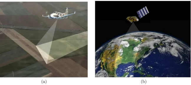
(a) (b)
Figure 1.1: Two main types of remote sensing. (a) Airborne and (b) space-borne remote sensing.
unsafe regions. It is used in most earth observation areas where it generally refers to the utilization of satellite- or aircraft-based sensor technologies to detect and classify objects on Earth. Therefore, the two main types of remote sensing includes airborne and space-borne remote sensing as shown in Figure 1.1. As can be seen from this figure, in the former, remote sensing data is obtained using the remote sensor on board of an airplane while in the latter, a satellite carries the imaging equipment. A remote sensor is an equipment that detects electromagnetic energy, measures it, and usually register it in an analogue or digital way. Remote sensors can be divided into two categories: passive and active. Figure 1.2 shows the schematic of these two types of remote sensors.
Passive remote sensors measure the energy that is naturally available. In the earth observation applications, the majority of the passive remote sensors detect the solar energy reflected back from the scene while the others measure the earth’s emitted energy. There are caveats related to these two types of passive sensors. Solar energy dependent-sensors fail to operate at conditions where there is not enough or is no sunlight such as night times, in regions of the world permanently covered under the clouds or parts of the globe where sun’s elevation is very low for most of the seasons resulting in unfavorable long shadows. On the other hand, the second type of passive sensors have difficulties
detecting earth’s emitted energy since this energy corresponds to the low frequency-waves carrying low energies which makes them hard to be detected. A camera which is used to take pictures in the sunlight (i.e., flash of the camera is not used) is a simple example of a passive sensor.
Figure 1.2: Active versus passive remote sensor. In passive remote sensing, Sun is often the source of energy whereas in active remote sensing, the airplane/satellite carries the energy source.
Different from the passive sensors, active sensors use their own source of energy for illuminating the object or scene of interest. In this case, electromagnetic energy is emit-ted through an energy source inside an airplane or a satellite and reflecemit-ted radiation is measured by the sensor. Active sensors can then be used in both day and night, do not depend much on the weather conditions and provide a controlled light signal. Moreover, active sensors are used to measure the reflectance at the wavelengths that are not ad-equately provided by the sun such as microwaves. A common camera which is used in a relatively dark room and uses its own flash (energy source) to illuminate the scene is a simple example of an active sensor. The most commonly used active sensors for collecting data in the earth observation domain (geospatial data) include radar [1], laser fluorosensor and a synthetic aperture radar (SAR).
Examples of remote sensing applications include military surveillance, deforestation observation [2–4], glacier change monitoring [5,6], agriculture [7], waste management [8], etc. The following are few specific examples of the usage of remotely sensed images of Earth [9]:
• Huge forest fires can be viewed from the space which enables rangers to see a bigger portion of the ground under the fire; so, making more effective plans compared to when the fire is observed only from the ground.
• Weather forecasting by the means of cloud tracking
• Watching for the erupting volcanoes
• City growth monitoring and tracking the changes in certain farmlands for years or even decades
• Ocean floor mapping
• Counting polar bears in satellite images to ensure sustainable population levels
• Marine life preservation by detection of the oil spills and predicting their movement directions.
1.1.2
Remote sensing mission examples
A lot of effort have been made in the last two decades to collect remote sensing data widely used in the Earth science applications. Hyperspectral infrared imager, HyspIRI, mission conducted by NASA (2007-present) for instance, studies the existing ecosystems on our planet and provides with precious information about ecosystem changes and natural catastrophes such as volcanoes, wildfires, and drought [10]. In order to meet its goals, the HyspIRI data acquisition system is equipped with a visible-to-short-wave-infrared (VSWIR) imaging spectrometer with the spectral range of 380-2510 nm with 10-nm spectral resolution and a multispectral imager ranging from 3-13µm containing 8 discrete bands covering the mid and thermal infrared (TIR) part of the electromagnetic (EM) spectrum. According to its final report in 2018, there are many potential applications related to the hyper and multi-spectral data obtained from the HyspIRI including but not limited to the following:
Catastrophes: Quantifying the possible dangers caused by volcanoes and wildfires
using the data collected by the TIR sensor. Since the TIR instrument works at the range of 3-13 µm and because of the fact that very hot objects emit energy at the wavelength of 4µm and thanks to the high spatial resolution of the TIR sensor, it is easy to detect pixels that correspond to active lavas or active fire burns (e.g. wildfires). Moreover, due to the capability of this sensor to measure a wide range of energy intensities, it would be possible to identify the most active lavas/fires.
Water Quality: The HyspIRI mission provides the hyperspectral images ranging
from the visible to shortwave infrared and multispectral thermal data that provides a valuable source of information enhancing the water quality monitoring. Observation of the optical characteristics of water by employing the hyperspectral imaging can be a powerful mean for water quality assessments especially for the water bodies that have been exposed to contaminants such as harmful algal blooms (HABs) [11] over the years. As a specific example of this application, we can name the HAB monitoring on the Great Lakes which is the largest source of freshwater worldwide and provides the drinking water for 40 million residents of the U.S. and Canada. The characteristics of the HyspIRI system (visible-shortwave infrared and thermal wavelengths) help improve the identification of the toxic bacteria related to HABs and also their spatial distributions through the Great Lakes’ surface water.
Another example of the missions with the goal of collecting hyperspectral data from the Earth is the hyperspectral imager suite (HISUI) mission [12]. HISUI is a spaceborne hyperspectral imaging system which has been established by the Japanese ministry of economy, trade, and industry (METI) as its forth spaceborne optical imaging project beginning in the year 2006 and scheduled to be launched for January 2020 through SpaceX’s Falcon-91(SpX-20) to be deployed on the international space station (ISS). One
of the mentioned potential functionality of the manufactured instrument (hyperspectral imager) will be applications such as oil resource exploration. The imaging system of
1Falcon 9 is a two-stage-to-orbit medium lift launch vehicle designed and manufactured by SpaceX
HISUI includes a reflective telescope and two spectrometers working in the near infrared and shortwave infrared (SWIR) regions of the EM.
HyspIRI and HISUI missions are just two examples of the many projects carried out in the area of remote sensing hyperspectral imaging. More projects are expected to be planned for the future due to the need of the human being to have more information about the phenomena occuring on our planet by the means of the irreplaceable data that spaceborne or airborne hyperspectral imaging systems can provide. The effort and cost of the missions such as HyspIRI and HISUI delivering the valuable source of information is well appreciated only in the presence of powerful hyperspectral and multispectral image analysis approaches. Currently, deep-learning based methods are the state of the art algorithms for classification of such data and even though there have been a large number of researches in this realm, there is still a lot to be explored.
1.2
Research problem
Motivated by the countless number of applications related to remote sensing tral images and the applicability of the artificial intelligence (AI) in processing hyperspec-tral data, In this study, we performed experiments on four hyperspechyperspec-tral image databases and proposed three new deep-learning based methods to carry out pixel-wise classification of these datasets.
1.2.1
Hyperspectral image classification
A typical hyperspectral image is composed of many images each taken at a specific wavelength. So, it can be imagined as a cube where the length and width of the cube corresponds to the spatial extent (number of pixels) of the 2-d image at each wavelength while its depth represents the number of spectral bands of the hyperspectral image. A typical hyperspectral dataset is shown in Figure 1.3. In HSI, imaging and spectroscopy
Figure 1.3: A sample hyperspectral image. This hyperspectral database was taken with Reflective Optics System Imaging Spectrometer (ROSIS) during a flight over Pavia Uni-versity, in northern Italy.
are combined to obtain a great source of spectral and spatial information of the scene. Because of the fact that different material own different spectral signatures, in an HSI, the type of the objects at each pixel can be identified using the spectral information while the spatial data provides their spatial distribution in the image. Hyperspectral imaging is explained in more detail in Section 2.1.
There are problems associated with hyperspectral image classification especially using deep neural networks: The large spectral size of the database which introduces a lot of tunable parameters to the model and the unavailability of adequate ground truth data to train the model effectively. Performing dimensionality reduction and data augmentation are two category of approaches to reduce the effect of these bottlenecks. In Chapters 3 and 5, we will propose two methods to deal with these problems. Moreover, since one important factor in HSI classification is to use the spatial information as effectively as possible, in Chapter 4, we propose a novel approach to extract spatial information to boost the classification accuracies.
The conventional and new approaches in hyperspectral image classification are de-scribed in Section 2.2.
1.3
Research contributions
This thesis is divided in six chapters and includes the following contributions:
• A new technique for hyperspectral image classification based on a combination of a supervised data dimensionality reduction method and a deep learning framework is proposed which results in high classification accuracies and smaller testing time.
• A new deep learning-based technique to perform pixel-wise classification of remote sensing hyperspectral scenes based on a novel spatial feature representation is pro-posed. We applied this proposed method on a new hyperspectral dataset, Surrey. This method improves the classification accuracies and the test time.
• A new approach for computing the distance transform image from an input hyper-spectral image is proposed.
• A simple new technique for augmenting the available ground truth data using a spectral perturbation method is proposed.
• A through search in the models’ hyperparameter space was performed to find the optimum values for these quantities.
Background and Literature Review
2.1
Background
Spectral imaging for remote sensing of the ground’s objects and features have become an active field of study among researchers. This technology as an alternative to the high-spatial resolution, large aperture satellite imaging systems has brought ease and convenience in the remote sensing domain. To have a better understanding of this tech-nology lets first see what the electromagnetic (EM) spectrum is.
EM spectrum is the term that describes the whole range of EM radiation. EM radiation can be represented by the means of waves or photons. Based on the wave theory, unless influenced by an outside object, light travels in a straight line and the energy it carries oscillates in a wave fashion. The two oscillating components of light include electrical energy and magnetic energy. A schematic of the EM spectrum is shown in Figure 2.1. As can be seen from this figure, EM spectrum is composed of different types of EM radiation including radio waves, microwaves, infrared light, visible light, ultraviolet light, X-rays and gamma-rays. In fact, visible light is the only part of the EM spectrum which can be sensed by human eyes and it only covers the small wavelength range between about 400 nm to 750 nm.
Visible spectrum
-rays X-rays UV IR Microwave Radio waves
Wavelength (m)
400 500 600 700
Wavelength (nm)
Figure 2.1: Electromagnetic spectrum
In the early applications of spectral imaging, only a small number of selected bands in the visible and infrared regions of the electromagnetic spectrum was used which in this case, it was called multi spectral imaging (MSI). Advanced spaceborne thermal emission and reflection radiometer (ASTER) [13] and land remote sensing satellite (Landsat) [14] are two of the most well-known MSI systems. In the newer version, HSI, hundreds of contiguous spectral bands are employed to identify various natural and human manu-factured materials. Visible light and infrared radiation are the most commonly used regions of EM spectrum in remote sensing applications. Airborne visible/infrared imag-ing spectrometer (AVIRIS) [15], designed by NASA at jet propulsion laboratory (JPL) in 1980s, is an excellent instance of an HSI system. Because of the valuable amount of information that HSI datasets can provide, they are used in many areas such as remote sensing [16–19], agriculture [20], food processing [21–23], face recognition [24], etc.
The concept of hyperspectral imaging is that for different materials the value of radiation that is reflected, absorbed, or emitted is a function of the wavelength. In hyperspectral imaging sensors, for each square pixel area in the scene composing of various materials and for a large number of consecutive spectral bands, the amount of the radiance is measured. Figure 2.2, shows the concept of hyperspectral imaging. Four major components of any remote sensing hyperspectral imaging system includes: the
Figure 2.2: Concept of hyperspectral imaging. A large area on the ground is being im-aged by an airborne/spaceborne imaging device covering a wide range of electromagnetic spectrum. Different reflectance values for the three sample materials in the scene depicts how different classes can be identified using their reflectance values.
radiation (or illuminating) source, the atmospheric path, the imaged surface, and the sensor [25]. In passive remote sensing, where the sun is often the main illumination source, what is measured by the sensor is the solar energy that has emitted from the sun, traveled through the atmosphere, interacted with materials on the earth’s surface and reflected back to the sensor. At this point, this measured energy is transformed into a digital form for further processing. The reflectance spectrum, or spectral signature of any material, is a function of the wavelength λ and is defined by (2.1)
reflectance spectrum(λ) = reflected radiation at band(λ)
incident radiation at band (λ) (2.1)
where the numerator is the reflected energy by the material and the denominator repre-sents the incident energy (energy received by the material) at different wavelengths [25]. It should be noted that solar energy is absorbed by the oxygen and water vapor in the at-mosphere at some specific wavelengths, called absorption bands, owning very poor signal to noise ratio. Therefore, in real applications, these bands are discarded.
electromagnetic wave to detect a single material uniquely, in real conditions where that single material is combined with other materials on the earth surface and being imaged through severe changeable atmosphere, it would be better to have many bands (features) than a few. In fact, having a large number of spectral bands makes it possible to apply statistical methods on the data composing of pixels each containing various material components [26].
2.2
Literature review
Since remotely sensed hyperspectral images can cover wide areas on the ground as well as provide reflection information at so many spectral bands, they provide a wealth of data for researchers and scientists. A lot of effort have been made to utilize the informa-tion hidden in remote sensing hyperspectral images as effectively as possible employing machine learning-based techniques. Traditional classifiers such as support vector ma-chine (SVM) classified each pixel using only its spectral information [27–29]. In other words in these methods, spectrum of each pixel was given to the classifier as the input feature vector. K-nearest neighborhood (KNN) and its variations are another types of HSI classification methods using only spectral information as the pixels’ features [30]. Researches depict that spectral information provide a useful source of information to perform the classification task with reasonable amount of accuracy. However, since the adjacent pixels in an HSI share similar spectral characteristics, combining the spectral and contextual spatial information help classify pixels with higher degrees of accuracy.
Early works on combining spectral and spatial information to classify spectral imagery data was devoted to multispectral images [31, 32]. Later, Pesaresi et al proposed a new
method to incorporate spatial information using morphological profiles (MPs) [33]. MPs of a gray-level image are obtained by applying a set of morphological operations called opening and closing by reconstruction by a structuring element (SE) of fixed shape and increasing size on the image such that some spatial details in the image are weakened while
some other are maintained. An extension of the MP called extended morphological profile (EMP) was proposed by Benediktsson et al [34] and Fauvel et al [35] to generalize the
idea to multi/hyper spectral images. In EMP, first principal component analysis (PCA) is applied on the input hyperspectral image to reduce the dimensionality of the data as well as band correlations. Then the MP method is applied on the first few principal components (PCs). Eventually, the MPs of all PCs are stacked together forming the final EMP structure. Definition of PCA, MP, and EMP are presented in Section 2.3.1, 2.3.5.1, and 2.3.5.2, respectively.
Although EMP could successfully model spatial information of a hyperspectral image, it had some drawbacks such as inability to model various spatial information due to the fixed shape of the SE in obtaining the MPs. Attribute profiles (APs) as an improvement to MPs was proposed by Dalla Mura et al [36] in 2010. APs of an image are a set of
profiles obtained by applying some attribute filters on the image. These attribute filters process the input image at different levels and by removing connected components (CCs) that do not satisfy a criterion related to the attribute. An attribute in that sense can be any measure computable on the connected components of the image. For example, the size of the connected components can be an attribute. APs are more powerful than the MPs in modeling the spatial information of an image since they process the input based on different attributes flexible in their definitions. Similar to EMP, the extension of APs was proposed by Dalla Mura et al [37] called extended attribute profile (EAP) to make
it applicable on hyperspectral datasets. In the case of employing multiple attributes the structure is called extended multi attribute profile (EMAP) [37]. Explanation of AP, EAP, and EMAP are given in Sections 2.3.5.3, 2.3.5.4, and 2.3.5.5, respectively.
Another class of techniques which combines spectral and spatial information together are composite kernel (CK) methods. In this type of methods, spectral and spatial in-formation of a target pixel are combined through kernel functions. In [38], authors considered some statistical measurements of the neighboring pixels of a target pixel such as their mean or standard deviation values at each spectral band as its spatial infor-mation. Then, they combined spectral and spatial data by the means of a family of
CKs satisfying the Mercer’s conditions and used SVM classifier on top to perform the classification. A new set of generalized CKs was proposed in [39] to combine spectral and spatial information together with no weight parameters. In order to compute the spatial feature vector prior to apply the kernel function, the authors used EMAP data structure and finally used the multinomial logistic regression (MLR) classifier to perform the classification. In [40], CKs along with extreme learning machine (ELM) is used to perform classification of HSI datasets employing joint spectral-spatial features.
Although all of the mentioned spectral-spatial feature extraction techniques could successfully deliver a representation of the two kinds of information existing in the hy-perspectral datasets, they are extremely hand-crafted. For example, in EMAP method, user needs to identify what type of attributes he wants to use. Neural network (NN) has found its way to solve regression or classification problems in many areas specifically image classification where HSI classification was no exception. In fact, a lot of researches in recent years concentrated on employing NN as an automatic feature representation technique in classification of hyperspectral images. To speak more specifically, it is deep neural network (DNN) that has been considered as the most popular technique for HSI classification (or any type of image classification in general) in the past few years thank to the development of powerful graphical processing units (GPUs) and the availability of more training data. Recently, several studies in the remote sensing field have used deep learning models in order to perform hyperspectral image classification [41–48]. Re-sults of these studies demonstrated superior performance of deep learning methods in hyperspectral image classification compared to the conventional approaches.
In [41] and [49], for the first time the concept of deep learning was used for hyper-spectral image classification. In [41], stacked autoencoder (SAE) was used as the deep network to extract deep features of each training and test pixel in the hyperspectral im-age. Three kinds of features were extracted and used for classification: spectral features, spatial-dominated features, and joint spectral-spatial features. In the case of spectral features, spectrum of each pixel is given to the network as input. In order to extract spatial-dominated features, first, PCA is applied on the whole hypercube to reduce the
spectral dimensionality. Then, a neighborhood around each pixel is determined and is converted in the form of a 1-D vector which will be the input of the network. Finally in the last case, spatial-dominated information of each pixel are concatenated to the spectrum of the pixel to form the joint spectral-spatial feature vector which is fed to the network. Having pre-trained the all layers in the SAE, in order to perform fine-tuning and classification, all layers are connected and a logistic regression classifier is put on the top of the network. The output results revealed that the proposed approach outper-formed the state of the art methods used for HSI classification. Motivated by [41], in [44], a new feature learning method, called contextual deep learning (CDL) is proposed. Sim-ilar to [41], spectral and spatial features are extracted before classification. However, unlike [41], this method reduces the features’ spectral dimensionality and extracts the spatial features at the same time. In order to perform classification, MLR was used.
In [43], in order to extract deep spectral-spatial information, an improved version of SAE called spatially updated deep auto-encoder was introduced. The first contribu-tion of this study was altering the energy funccontribu-tion of each auto-encoder to ensure that correlation between samples is preserved while encoding them. Next, in order to take spatial information into account, a feature updated layer is embedded after the hidden layer which replaces each feature with an average value of the features extracted from the pixels in the neighborhood of the target pixel. In order to deal with not having enough training samples and also smooth the classification result, the authors introduce collab-orative representation based classification approach [50] into HSI classification domain to obtain an output vector (whose size equals to the number of classes) for each target pixel whose elements express the probability of belonging the pixel to each category. The final smoothed classification map was obtained by solving maximuma posteriori (MAP)
probability segmentation problem [51]. In [48], EMAP features with sparse autoencoder are used to classify three very high resolution (VHR) multispectral datasets. They have used a one layer SAE and employed area (a) and the standard deviations of the pixels in-side the connected components (s) as the attribute filters. Also, they used two threshold values for each attribute.
In [42, 46, 52], the task of hyperspectral image classification is performed using deep belief network (DBN) where restricted Boltzmann machine (RBM) is employed as the building block of the DBN. In [52], a DBN (with two hidden layers) extracts spectral-spatial features of the pixels in the hypercube such that first, the spectral dimensionality of the hypercube is reduced using PCA and only first three principal components are retained. Next, a 3D patch of size 7x7x3 around each training sample (pixel) is formed which was later vectorized and was given to the the network as input. Just like SAE, DBN is trained in a layer-wise manner. The final layer of the DBN consisted of a logistic regression (LR) classifier. In 2017, the concept of using grouped features was proposed by Zhouet al. [46]. Their method, called group belief network (GBN), adaptively diminishes
the weights of the connections which correspond to the irrelevant spectral bands. Similar to DBN, the proposed GBN is constructed of stacked RBMs; however, the bottom layer of the DBN is replaced by a modified version of an RBM named as Group-RBM (GRBM). The GRBM has the capability of managing grouped features. Proposed GBN-based HSI classification method has been applied on three HSI datasets and compared to DBN the segmentation results have been slightly improved.
Some recent studies have used convolutional neural network (CNN) as the deep net-work structure in order to extract spectral and spatial information both in supervised and unsupervised manners [45,47,53–58]. [53] considers each sample vector (sample spec-tra) as a 2D image; therefore, the input of the network is the spectral signature of each pixel. Structure of the CNN used in this study consists of a convolutional layer (C1), a max-pooling layer (M2), a fully connected layer (F3), and the output layer. Although the resulting classification accuracies showed the capability of the CNN in hyperspectral image classification, maximum overall accuracy of 92.6% implies that results could be further improved. Unlike [53] which does not use spatial correlation between samples for classification of the hyperspectral data, in [45], Zhaoet al. proposed spectral-spatial
fea-tures by employing balanced local discriminant embedding (BLDE), an extension of LDE algorithm introduced in [59], for reducing the spectral dimension of the input data and a CNN for spatial feature extraction. In order to extract spatial features of pixels, first, the
dimension of the original data (hypercube) is reduced along the spectral dimension using BLDE and only first few principal bands are kept. Next, a squared patch around each training pixel is formed. These patches are used as training data set for training the CNN in a supervised manner. The features in the last layer of the CNN framework are flat-tened and form the spatial feature vectors. By denoting zi as the spectral feature andoi
as the spatial feature of the unknown test samplexi where the former feature is obtained
using the BLDE method and the latter feature is computed by the trained CNN (on the training patches), the final feature for the test sample is obtained by concatenating these features as [zi,oi]. In 2017, Li et al. dealt with the small number of training samples
by building a Pixel-Pair model using available training samples [47]. The procedure is as follows: having M training samples of C different classes and expressing each training sample as {xi, yi} where xi is the training sample and yi is its corresponding label, for
increasing the number of labeled training samples any combination of two samples of all classes is randomly chosen and is calledSij whereSij = [xi xj]. If the two samples are
drawn from the same class, Sij will also have the same class label as theirs. However, if
they belong to different classes, the label of 0 will be assigned to Sij. [47] resembles the
approach proposed in [45] in that they both take advantage of spatial features as well as spectral information of the pixels. However, in [47] the incorporation of the spatial information is done in the test phase through introducing the ”Joint Classification With Voting Strategy”. This voting strategy is based on the fact that neighboring pixels belong
to the same class with a high probability. In the test step, each test sample is also com-bined with its neighbors to form pixel-pair samples and the target pixel will be assigned to the class to which the majority of its neighbors belong to.
In [54], in order to exploit spectral and spatial information, a 3D-CNN has been designed. This architecture can extract both spectral and spatial information simul-taneously because it forms a small 3D window (patch) around the target pixel in the hypercube and feeds as input this 3D patch to the network. After several convolutional and pooling layers the extracted features will be in the form of a vector which contains deep spectral and spatial information of the target pixel. This network can have fewer
trainable parameters but the computation cost is highly increased due to the convolution along spectral bands. The approach used in [55] for extracting the spectral and spatial information simultaneously from the data hypercube is similar to [54]. In other words, a 3D patch (tensor) around each target pixel is formed which contains both spectral and spatial information. However, unlike [54] which feeds these 3D tensors to the CNN as input directly, in [55] Randomized PCA (R-PCA) is applied on each 3D tensor in order to reduce the dimensionality of the input data. The proposed CNN also differs from the CNN used in [54] and also from a conventional CNN in that there is no pooling layer in the structure of the CNN.
2.3
Machine learning and image processing
Machine learning as one of the sub-categories of artificial intelligence (AI), is the science of automatically finding the hidden patterns in the data without human interventions. The fundamental requirement for developing a machine learning-based model is some sample data called training data used to train the model. After the model is trained using the
the training data, it will be able to make predictions or decisions on the new unseen data called testing data. The important concept of machine learning is that computers
are not programmed explicitly to perform a task, rather are taught to learn for them-selves and make decisions from what they have already seen (training data). Machine learning algorithms falls within the two main categories of supervised and unsupervised methods [60]. In supervised methods, training data includes data points with their la-bels while in unsupervised approaches lala-bels are not given to the model during training. In the following subsections, we introduce some of the machine learning methods from both categories which we will refer to later in this thesis. Furthermore, in Section 2.3.5 we describe a morphological-based image processing technique used to extract spatial information from input images.
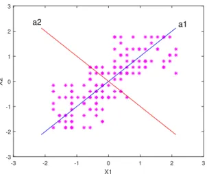
-3 -2 -1 0 1 2 3 X1 -3 -2 -1 0 1 2 3 X2 a1 a2
Figure 2.3: A toy example showing the directions of maximum variance in the data obtained by the PCA algorithm
2.3.1
Principal Component Analysis
PCA as a popular dimensionality reduction (DR) method has been introduced by Karl Pearson in 1901 [61] and has been used frequently in the literature in many fields ever since. This method searches for the most accurate data representation in a lower dimen-sional subspace composed of the uncorrelated linear combinations of the original variables called principal components. What PCA does is in fact, mapping the input data to the dimensions along which data vary the most; so, preserving the largest variances in the data. A toy example of applying the PCA algorithm on a sample of 2 dimensional points is shown in figure 2.3. As can be seen from this figure, a1 anda2 point to the directions
of the largest and the second largest variances in the dataset, respectively.
Suppose we have a data set composed of N,pdimensional samples. We can show the aforementioned efficient linear combinations of the original variables (PCs) as follows
Z1 =a11X1+a12X2+...+a1pXp =aT1X Z2 =a21X1+a22X2+...+a2pXp =aT2X ...
Zp =ap1X1+ap2X2+...+appXp =aTpX
(2.2)
where Zi is the ith principal component, ai represents the ith loading vector. Also, X
is a p-dimensional vector representing a point in a p-dimensional space. In the PCA algorithm, these PCs are computed through the following process:
Define the first principal component of the sample X = (X1, ..., Xp) by the linear
transformation Z1 =aT1X = p X i=1 a1iXi (2.3)
where the vector a1 is chosen such thatvar(Z1) is maximized.
Similarly define the kth PC of X according to (2.4)
Zk=aTkX = p
X
i=1
aikXi k = 1, .., p (2.4)
where vectorak is chosen such that the following conditions are met:
1. var(Zk) is maximized
2. cov[Zk, Zl] = 0 for k > l≥1
3. aT
kak = 1
The above conditions leads to following properties of PCA:
• var(Z1)≥var(Z2)≥...≥var(Zp)≥0
cov[Zl, Zm] = 0 and aTl am = 0 for l6=m
• Preservation of the total variance:
Pp
i=1var(Zi) =
Pp
i=1var(Xi)
The last property notes that there are the same amount of variance (information) in the whole set of PCs as there are in the original set of data. However, since we are interested in reducing the dimensionality of the input data, we only keep the first few PCs which contain the most information of the original data. It has been mathematically proven that the loading vectors that meet above requirements are in fact, the eigenvectors of the covariance matrix of the original points in the dataset [62].
Let’s show the eigenvalues and the corresponding eigenvectors of such a covariance matrix with λi and ei, respectively, where i is the index of these eigenvalues/vectors.
Considering equation (2.2) and the fact that the desired loading vectors in this equation are the eigenvectors ei, we can rewrite them as follows:
Z1 =e11X1+e12X2+...+e1pXp =eT1X Z2 =e21X1+e22X2+...+e2pXp =eT2X ...
Zp =ep1X1 +ep2X2+...+eppXp =eTpX
(2.5)
Also, it can be proven that for each Zk:
var(Zk) =λk =eTkSek (2.6)
whereS is the covariance matrix of the variables of the original dataset. In other words, thekth largest eigenvalue ofS is the variance of thekth PC and thekth largest fraction of the variation in the points of our dataset is preserved by this PC. It should be noted that in many applications, the true covariance matrix is not available so, what S represents in these equations is the sample covariance matrix of the set of given data points formed
in an N ×pmatrix. In equation (2.5), Z1 toZp are the pPCs of one observation in the
dataset (one row of the matrix of the input data of size N ×p). Equation (2.7) can be used to compute the PCs for all N observations in the dataset:
ZN×p =XN×pEp×p (2.7)
where each row of matrix X is an observation of size 1×p, E is a p×p matrix whose columns contain the p (normalized) eigenvectors of the covariance matrix S, and Z is the PC matrix whose jth row contain the PCs of the jth observation in X.
2.3.2
Linear Discriminant Analysis (LDA)
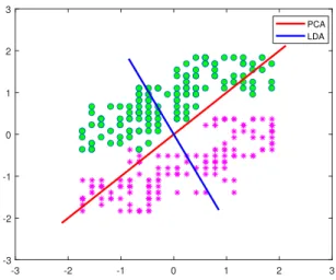
The most common usage of LDA is dimensionality reduction. This method was first introduced by Ronald A. Fisher in 1936 [63] as the feature extraction step for discrimi-nating between two classes of flowers. In 1948, a generalized version of this method called multi-class ”Linear Discriminant Analysis” or ”Multiple Discriminant Analysis” was in-troduced by C. R. Rao for a multiple class problem [64]. Although this DR method is very similar to the PCA algorithm, LDA is a supervised approach. In other words, we use class labels while reducing the dimension of the data and try to preserve as much of the class discriminatory information as possible. In that sense, the main objective of LDA method is projecting data into a lower dimensional subspace such that class-separability gets maximized. Figure 2.4 shows a toy example of the difference between PCA and LDA algorithm for two-dimensional data divided into two classes. As can be seen from this figure, PCA projects data into the direction of the maximum variance in the data regardless of their labels wheres LDA tries to find direction of the most variation of the data points while maintaining class separability at the same time.
Considering X as a dataset consisting of N p-dimensional samples with Ni samples
in each of theC classes each denoted by wi, LDA searches for a transformation function
-3 -2 -1 0 1 2 3 -3 -2 -1 0 1 2 3 PCA LDA
Figure 2.4: A toy example showing the best projection directions suggested by PCA and LDA algorithms.
class discriminatory information of the data. Let’s start with the two class problem and then generalize it to the C-classes case.
2.3.2.1 Two-classes case
Let’s say we have a database of p-dimensional samples x = [x1, x2, ..., xp]
T, where
N1 and N2 of those samples belong to classes w1 and w2, respectively. The objective is to find the transformation a in (2.8) that maps data from the original space x into the lower-dimensional subspace y while preserving the maximum class separability in this new subspace.
y=aTx (2.8)
where a= [a1, a2, ..., ap]T.
Since we have a two-class problem (i.e., C=2), y will be a one-dimensional space, so, each original vector x will be mapped to a scalar. In order to find a, we need to specify a separability measure between the projected samples. The approach proposed by Fisher [63] was to maximize the ratio of the difference of the two classes’ means (between-class variance) normalized by a term which is a function of the within-(between-class variation,
called scatter according to 2.9 J(a) = |µe1−µe2| 2 e s2 1+es 2 2 (2.9) where µ˜i and sei
2 are the mean and the within-class variation of the samples of class wi
having been mapped to the new subspace y, respectively. µei can be calculated according
to (2.10) e µi = 1 Ni X y∈wi y= 1 Ni X x∈wi aTx= a T Ni X x∈wi x=aTµi (2.10)
where µi is the mean of samples in class wi in the original p-dimensional space. In
fact, the numerator in (2.9), states how far the mean of the projected samples in the two classes are from each other. The equation for each class’s scatter is the same as its variance e si2 = X y∈wi (y−µei)2. (2.11) We can define se1 2
+se22 as a measure of the within-class variation of the projected samples and it is called the within-class scatter of the projected samples.
The objective now is to maximize the energy function in (2.9). In other words, we would like to obtain a projection where samples of the same class are as close as possible to each other while as further apart as possible from samples of the other class. To find the optimal transformation that maximizes the energy function, we need to rewrite equation (2.9) as a function of a. Substituting equation (2.10) into the numerator of the energy function results in
(µe1−eµ2)
2
= aTµ1−aTµ22 =aT (µ1−µ2) (µ1−µ2)Ta
=aTSBa=SeB
(2.12)
whereSB is a matrix and is called the between-class scatter of the samples in the original
To have the within-class scatter matrix of the projected samples in terms ofa as well, we can use equation (2.11) as follows
e si2 = X y∈wi (y−µei)2 = X x∈wi aTx−aTµi2 = X x∈wi aT (x−µi) (x−µi)Ta =aTSia (2.13)
where Si is a measure of the variation of original samples in class wi. We can rewrite
the denominator of the energy function in (2.9) (which is in fact the within-class scatter of the projected samples) as follows
e
s21+es22 =aTS1a+aTS2a=aT (S1+S2)a=aTSWa =SeW (2.14)
Finally, equation (2.9) can be reformulated as a function of the transformation vector a, SB, and SW: J(a) = |µe1−µe2| 2 e s21+se22 = aTS Ba aTS Wa (2.15)
The transformation vector that maximizes J(a), a∗ is called Fisher’s linear discrimi-nant and it turns out that it is in fact the eigenvector of the following matrix [63]:
SX =S−W1SB (2.16)
2.3.2.2 C-classes case
In the case of having C classes, the maximum dimension of the projected samples can be C −1. So in this case, our objective will be to find the C −1 projection vectors
that result in the maximum between class and minimum within-class variances. Let’s populate these projection vectors in a matrix of size p× (C − 1) called A. We use equation (2.17) to project the entire samples in the original p-dimensional space to the
new (C−1)-dimensional feature space.
Y =ATX (2.17)
where X is a p×N matrix including the original dataset and Y is a matrix of size
(C−1)×N consisting of the projected samples in the lower dimensional space.
To find the within-class variance for the C classes case, similar to the previous case we need to add the scatter matrices of all the C classes:
SW = C X i=1 Si = C X i=1 X x∈wi (x−µi) (x−µi)T (2.18)
where µi is the mean of the original samples in class wi.
To find the between-class scatter of original samples, SB, we use the mean of all
samples in the dataset, µaccording to (2.19):
SB = C X i=1 Ni(µi−µ) (µi−µ) T (2.19)
Similarly, the within and between- class scatter matrices for the projected samples (SeW and SeB, respectively) can be expressed in equations (2.20) and (2.21), receptively.
e SW = C X i=1 e Si = C X i=1 X y∈wi (y−µei) (y−µei)T (2.20) e SB = C X i=1 Ni(µei−µe) (µei−µe) T (2.21)
where µei and µe are the mean of projected samples of class wi and the mean of all
It should be noted that equations (2.12) and (2.14) hold for the C-classes case as well. Since in the case of having more than two classes,SeW and SeB are matrices rather than
scalar values, we use their determinant value in the equation of the energy function.
J(A) = SeB SeW = ATSBA ATSWA (2.22)
The desired matrix, A∗, is the one that maximizes the energy function in (2.22). It can be mathematically proven that similar to the two-classes case, such A∗ matrix is composed of the eigenvectors of the following matrix
SX =S−W1SB. (2.23)
A∗is ap×(C−1)matrix whose columns are the eigenvectors of matrixSX in equation
(2.23) and are located in an descending order such that the jth column corresponds to the jth largest eigenvalue of SX.
2.3.3
Artificial neural networks (ANN)
Artificial neural networks are machine learning based classifiers whose architecture is inspired by the way human brain works. An ANN is composed of connected units called artificial neurons which are similar (but not the same) as human biological brain neurons. Each neuron has some main components: cell body, dendrites, and axon. Cell body is the main computational unit of a neuron. Dendrites act as input wires which receive input data from other neurons. Each neuron may own thousands of these input receivers which are usually short in length. Axons, as opposed the dendrites, are the neuron’s output wires which send information signals to other neurons and can break into thousands of branches at the end called axon terminals. Axons own a single long shape which can be up to one meter in length.
2.3.3.1 Single layer neural network (perceptron)
In an ANN, instead of a neural signal, what each neuron receives is a sum of weighted numbers/inputs. This sum will then go through a non-linear function to provide the neuron’s output. Figure 2.5 shows a graphical representation of a single layer neural network including only one hidden neuron. In fact, such a network performs like a perceptron, a binary linear classifier. The output of a single layer NN can be formulated as (2.24): y=f p X j=1 wjxj+b ! (2.24)
where xj is the jth element of the input vector x and wj is the corresponding weight
between that input and the hidden neuron. Also, b represents a bias value. f is the neuron’s non-linear activation function.
Activation functions introduce nonlinear properties to our model and let the network learn complex mappings from the input to the output. In fact, we can consider ANN as universal function approximator which is capable of learning any function provided
that it contains nonlinear activation function. A neural network without activation func-tion resembles a linear regression model which is not capable of modeling real complex nonlinear relationships between the input and output of the network, so, fails to perform properly in real applications. Besides the nonlinear property, an activation function must be differentiable. The need for this property will be explained in Section 2.3.3.2. Figure 2.6 shows the most commonly used activation functions: sigmoid or logistic, tangent hyperbolic (tanh), and rectified linear unit (ReLU). What follows is a brief description
of these functions.
Sigmoid or logistic activation function: This function is defined by (2.25)
σ(z) = 1
1 +e−z (2.25)
x2 x3 xp x1 ... 1 w1 w2 w3 wp b
y
Figure 2.5: Graphical representation of a single layer NN with only one hidden neuron which functions similar to a perceptron.
-8 -6 -4 -2 0 2 4 6 8 z 0 0.5 1 (z) (a) -3 -2 -1 0 1 2 3 z -1 0 1 tanh(z) (b) -8 -6 -4 -2 0 2 4 6 8 z 0 2 4 6 8 ReLU(z) (c)
Figure 2.6: Several activation functions. (a) Sigmoid, (b) tanh, (c) ReLU.
the corresponding weights W = [w1, w2, ..., wp], bias value b, and the sigmoid activation
function can be represented as (2.26)
σ(z) = 1
1 +e−(Ppi=1xiwi+b)
. (2.26)
As can be seen from Figure 2.6a the output of the sigmoid function is bounded between 0 and 1 which makes it especially useful when we expect our model to predict the probability of a class (or event) to happen. This function is differentiable at all points which is one of the reasons behind its popularity in ANN applications. However, the drawback of using this sigmoid function is that since for the majority of the x domain its derivative has a very small value close to zero it can lead to the vanishing gradient
Tanh activation function: This function is the ratio between the hyperbolic sine
and the cosine functions and is defined as
tanh(z) = e
z−e−z
ez+e−z (2.27)
wherez is the weighted sum of inputs to the neuron. The shape of this function is quite similar to the sigmoid function (see Figure 2.6b) but it is bounded between -1 and 1. Similar to the sigmoid function, tanh is differentiable at all points.
ReLU activation function: This activation function has become popular recently
especially in CNN applications. Considering z as the input and f(z) as the output of
this function, the relationship between these two can be formulated as (2.28)
f(z) = z if z ≥0 0 otherwise. (2.28)
As can be seen from Figure (2.6c), it is differentiable at all points. Also, since the gradient of this function is equal to one for the positive inputs, it solves the vanishing gradient problem making it a popular activation function. Nonetheless, ReLU has some drawbacks as well. First, it should only be used in hidden layers of a NN and for a classification problem, in the output layer, Softmax function must be employed. Second,
using the ReLU function, all the negative values as inputs of the function will be mapped to zero immediately which decreases the ability of the model to fit or train from the data properly.
2.3.3.2 Multi layer neural network
To obtain a more powerful classifier than a perceptron with more complex decision bound-aries, multiple perceptrons are combined and function together. They are arranged in layers such that each neuron takes the sum of its weighted inputs, apply the activation