Linking credit risk premia to the equity premium

econ

stor

Der Open-Access-Publikationsserver der ZBW – Leibniz-Informationszentrum Wirtschaft

The Open Access Publication Server of the ZBW – Leibniz Information Centre for Economics

Nutzungsbedingungen:

Die ZBW räumt Ihnen als Nutzerin/Nutzer das unentgeltliche, räumlich unbeschränkte und zeitlich auf die Dauer des Schutzrechts beschränkte einfache Recht ein, das ausgewählte Werk im Rahmen der unter

→ http://www.econstor.eu/dspace/Nutzungsbedingungen nachzulesenden vollständigen Nutzungsbedingungen zu vervielfältigen, mit denen die Nutzerin/der Nutzer sich durch die erste Nutzung einverstanden erklärt.

Terms of use:

The ZBW grants you, the user, the non-exclusive right to use the selected work free of charge, territorially unrestricted and within the time limit of the term of the property rights according to the terms specified at

→ http://www.econstor.eu/dspace/Nutzungsbedingungen By the first use of the selected work the user agrees and declares to comply with these terms of use.

zbw

Berg, Tobias; Kaserer, Christoph

Working Paper

Linking credit risk premia to the equity

premium

CEFS working paper series, No. 2008-01

Provided in cooperation with:

Technische Universität München

Suggested citation: Berg, Tobias; Kaserer, Christoph (2008) : Linking credit risk premia to the equity premium, CEFS working paper series, No. 2008-01, http://hdl.handle.net/10419/48436

WORKING PAPER SERIES

Center for Entrepreneurial and

Financial Studies

Working Paper No. 2008-01

Linking Credit Risk Premia to the Equity Premium

TOBIAS BERG

CHRISTOPH KASERER

Technische Universit¨at M¨unchen Arcisstr. 21 D-80290 Munich Germany +49 89 289 25489 (Phone) +49 89 289 25488 (Fax) tobias.berg@wi.tum.de Christoph Kaserer†

Technische Universit¨at M¨unchen

Arcisstr. 21 D-80290 Munich Germany +49 89 289 25490 (Phone) +49 89 289 25488 (Fax) christoph.kaserer@wi.tum.de Jan. 06th, 2008 ∗

Tobias Berg, Department of Financial Management and Capital Markets, Technische Universit¨at M¨unchen

†

Prof. Christoph Kaserer, Department of Financial Management and Capital Markets, Technische Universit¨at M¨unchen

Abstract

Although the equity premium is - both from a conceptual and empirical perspective - a widely researched topic in finance, there is still no consensus in the academic literature about its magni-tude. In this paper, we propose a different estimation method which is based on credit valuations. The main idea is straigtforward: We use structural models to link equity valuations to credit valuations. Based on a simple Merton model, we derive an estimator for the market Sharpe ratio. This estimator has several advantages. First, it offers a new line of thought for estimating the equity premium which is not directly linked to current methods. Second, it is only based on observable parameters. We do neither have to calibrate dividend or earnings growth - which is usually necessary in dividend/earnings discount models - nor do we have to calibrate asset values or default barriers - which is usually necessary in traditional applications of structural models. Third, it is robust to model changes. We examine the model of Duffie/Lando (2001) which is one of the most sophisticated structural models currently discussed in the literature -to show this robustness.

In an empirical analysis we have used CDS spreads of the 125 most liquid CDS in the U.S. from 2003 to 2007 to estimate the equity premium. We derive an average implicit market Sharpe ratio of appr. 40%. Adjusting for taxes and other parts of the credit spread not attributable to credit risk yields an average market Sharpe ratio below 30%. This confirms research on the equity premium, which indicates that the historically observed Sharpe ratio of 40-50% - correspond-ing to an equity premium of 7-9% and a volatility of 15-20% - was partly due to one-time effects. In addition, our research can be used to explain empirical findings about credit risk premia, which are usually measured as the ratio of risk-neutral to actual default probabilities. We show that the behavior of these ratios can be directly inferred from a simple Merton model and that this behavior is robust to model changes.

1

Introduction

Risk premia in equity markets are a widely researched topic. The risk premium in equity markets is usually defined as the equity premium, e.g. the excess return of equities over risk free bonds. The literature discusses three different ways for the measurement of the equity premium: Models based on historical realizations, discounted cash-flow models and models based on utility functions. While historical averages have long dominated theory and practical applications, current research suggests an upward bias, e.g. the ex post realized equity returns do not correctly mirror the ex ante priced equity premium.1 In the U.S., historical averages have been around 7-9% depending on the time horizon and methodology (arithmetic/geometric) used.2 Discounted cash-flow models have become more popular recently, but are also subject to debate, in particular for their rather high sensitivity to forecasts with respect to dividend- or earnings growth rates. Estimations based on such models yield implied equity premia in the range from 3%-5%.3 Although approaches based on utility functions have been subject to intensive debate in the academic literature4, its use in practical applications is currently of minor importance.

The risk aversion of investors influences credit prices and returns as well. As an example, we have looked at CDS contracts of A-rated obligors in the CDS-index CDX.NA.IG from 2003-2007. The average 5-year CDS spread has been 37 bp, whereas the average annual expected loss is less than 10 bp. Therefore, these 5-year CDS investments yield an average return of appr. 28 bp above the risk free rate, as can be seen from table 1. In absolute terms, this premium increases with decreasing credit quality (i.e. the expected net returns increase with increasing ’riskyness’). Mea-sured relative to the expected loss (or the actual default probability) it decreases with declining credit quality. Over the last years, research about this default risk premium has developed, but there has not yet emerged consensus on the methodology for measuring this default premia.5

We use structural models of default to convert credit spreads into an equity premium. Speci-fying a specific structural model, one can derive the risk neutral and the actual default probability. Used the other way around, the difference between risk neutral and actual default probability yields the dynamics of the asset value process, in particular the asset Sharpe ratio. Together with the asset correlation, we are then able to derive the market Sharpe ratio.

The estimator for the market Sharpe ratio derived in this paper has three important charac-teristics, which make it very convenient for our purpose. First, it is only based on observable parameters, i.e. risk neutral and actual default probabilities, the maturity and the equity correla-tion. The risk neutral default probability and the maturity can be derived from bond prices or CDS

1

Among other things, this can be explained by survivorship bias, risk premium volatility, enhanced diversification possibilities, interest rate level and state of the economy; cf. for example Claus/Thomas (2001), Illmanen (2003), Fama/French (2002).

2

Cf. for example Claus/Thomas (2001) and Fama/French (2002) for a discussion and Ibbotson (2006) for historical data.

3

Cf. for example Claus/Thomas (2001), Fama/French (2002) and Illmanen (2002) for an overview.

4_{This debate is mainly based on the so called ’Equity Premium Puzzle’ put forward by Mehra/Prescott (1985).}

Cf. Mehra (2003) for an overview about different utility based approaches including alternative preference structures, disaster states, survivorship bias and borrowing constraints.

5

Rating grade Average 5-y-CDS-mid (bp) Average 5-y-EL p.a. (bp) ∆ (bp) Q-to-P AA 31.53 5.23 26.30 6.03 A 37.37 9.17 28.20 4.07 Baa1 48.43 14.60 33.83 3.32 Baa2 56.91 22.00 34.91 2.59 Baa3 68.51 33.17 35.34 2.07

Table 1: Credit risk premia for 5-year CDS (Index CDX.NA.IG). ∆(bp): Difference in bp between 5-year-CDS spread and 5-year-EL p.a. Q-to-P: ratio of CDS spread to EL p.a., equals the ratio of risk neutral to actual default probabilities.

spreads, the actual default probability from ratings6 _{and the correlation from equity prices. Unlike}

other applications of structural models, we do neither have to calibrate the asset value process nor the default barrier. Second, the estimator is robust with respect to model changes. We examine a classical first passage time model and the Duffie/Lando (2001) model, which incorporates strategic default and unobservable asset values. By introducing an adjustment factor capturing the difference between the Sharpe ratio estimation in the Merton model and the Sharpe ratio estimation in the Duffie/Lando (2001) model, we show that the adjustment factor is close to one for all investment grade obligors. Third, the estimator is robust with respect to noise in the input parameters. As an illustration, we look at a model-based 5-year spread of a BBB-rated obligor. This credit spread is 73 bp for a company Sharpe ratio of 10%, it is 280 bp for a company Sharpe ratio of 40% (cf. subsection 2.1 for a detailled analysis). This difference indicates that the common noise in the data7 will not significantly reduce the possibility to extract the Sharpe ratio out of credit spreads. Mathematically, the sensitivity of the model-based credit spread with respect to the Sharpe ratio is ’high’ compared to other noise in the data.

We have applied our Sharpe ratio estimator to all NYSE-listed companies in the investment grade CDS index CDX-NA.IG from 2003 to 2007. The risk neutral default probability was derived from CDS spreads, EDFs (expected default frequencies) from KMV were used as a proxy for the actual default probability. We estimated the implied market Sharpe ratio to be about 42% and the com-pany Sharpe ratio to be about 20%. Adjusting for tax effects results in a market Sharpe ratio of 32% and a company Sharpe ratio of 16%. Using Moody’s ratings instead of EDFs shows similar results, i.e. a market Sharpe ratio of 39% before and 29% after tax adjustments. This corresponds to an equity premium of 4.5% - 6%8 and therefore confirms former research, that the historical equity premium is upward biased. We also show, that for higher rating grades, only 50-70% of the CDS spreads can be explained by credit risk.9 Reducing the CDS spreads by the amount not due to credit risk results in even lower equity premium estimates.

6_{We use EDFs (expected default frequencies) from Moody’s KMV and Moody’s ratings.} 7

E.g. bid-ask spreads, liquidity effects and inaccuracies in determining the actual default probability.

8_{Assuming a market volatility of 15-20%.} 9

This is partly in contrast to research by other authors. Huang/Huang (2005) analyzes bonds and comes to the conclusion, that for Aa (A) rated obligors only 9 % (10%) of the spread can be explained by credit risk. The difference to our analysis is due to three effects. First, we only use the most liquid CDS in the U.S. market, which should decrease the part of the spread attributable to liquidity. Second, the CDS spreads observed in our sample are consistently lower than the bond spreads observed by Huang/Huang (2005). We observe average 5-year CDS spreads of 26/34/50 (Aa/A/Baa) compared to 4-year bond spreads of 65/96/158 by Huang. Third, we use a model with unobservable asset values which increases theoretical credit spreads especially for high rated obligors.

In addition, our method allows for an extraction of the market’s risk attitude over time. We find, that the implicit Sharpe ratio predominantly varied between 30% and 50% (before adjusting for tax effects) from 2003-2007 with peaks in 2005 and mid 2007.10

The remainder of the paper is structured as follows. Section 2 describes the theoretical frame-work for credit risk premia based on asset value models including a discussion of the impact of different asset models on the widely used ratio of risk neutral to actual default probabilities (’Q-to-P-ratios’). We examine a classical Merton model, a first passage time model and a model based on unobservable asset values as proposed by Duffie/Lando (2001). In our perspective, using a model with unobservable asset values is crucial, since only these models are able to explain credit spreads observed in the markets and yield a default intensity, which constitutes the basis of modern credit pricing models. Section 3 describes our data and contains a discussion of our empirical results. Section 4 draws a conclusion.

2

Model setup

This section discusses the theoretical framework for extracting risk premia from CDS spreads. The basic idea is to use structural asset models to derive a relationship between risk neutral and actual default probability. Empirically, most structural models perform poorly.11 _{One of the main reasons}

is the calibration process usually needed to specifiy structural models, e.g. determination of lever-age, asset volatilities etc. In contrast to mainstream literature12, we do however not aim to derive actual and risk neutral default probabilities from structural models. We are simply interested in the relation between risk neutral and actual default probabilities. Hence, we simply assume, that there exists a structural model yielding the correct actual default probability and from there derive the risk neutral default probability. It is therefore not necessary to perform the calibration process that is usually needed.

Subsection (2.1) starts with the classical Merton model. We derive a simple Merton estimator for the market Sharpe ratio. This estimator is only based on observable parameters, i.e. the risk neutral and actual default probability, the maturity and equity correlations. Subsection (2.2) ex-pands the framework to a simple first passage time model. The results do not materially differ from to the simple Merton framework as long as the asset volatility is above 10%. Asset volatilities below 10% are generally only observed for financial services companies. Subsection (2.3) expands the approach to the Duffie/Lando (2001) model and confirms the results derived in the simple Merton model for all investment grade companies.

10_{Some authors analyze the risk aversion based on the ratio of risk neutral to actual default probabilities. Since}

these ratios are also largely driven by development of the average rating grade in the sample, we think that the results do not mirror the risk attitude correctly.

11

Cf. Sch¨onbucher (2003) for an overview.

12

Huang/Huang (2005), Bohn (2000) and Delianedis/Geske (1998) use a similar approach. Our approach differs though in at last three ways: First, we explicitly focus on models with information uncertainty; second, we use CDS spreads, which should be less sensitive to liquidity distortions; third, we are - to our best knowledge - the first who directly aim to extract the risk attitude out of credit prices via a Sharpe ratio estimation.

2.1 Sharpe ratio estimation in the Merton framework

In this subsection we derive an estimator for the Sharpe ratio based on a simple Merton model. This estimator is based on the actual and risk neutral default probability, the maturity and the equity correlation of the respective company. Although based on a structural model, we can omit the calibration process usually needed for structural models (e.g. default barrier, asset volatility). In contrast to dividend-/cash-flow discount models, we do not have to calibrate earnings/dividends and their respective growth rates.

Structural models for the valuation of debt and the determination of default probabilities are already mentioned in Black/Scholes (1973). The Merton framework presented in this subsection is based on Merton (1974), who explicitely focusses on the pricing of corporate debt. In this framework a company’s debt simply consists of one zero-bond. Default occurs if the asset value of the company falls below the nominal value of the zero bond at the maturity of the bond. A company can therefore only default at one point in time, which obviously poses a simplification of the real world. The assetsVt are modelled as a geometric Brownian motion with volatilityσ and drift µ=µV (actual drift) and r (risk neutral drift) respectively, i.e. dVtP =µVtdt+σVtdBt and

dV_tQ=µVtdt+σVtdBt, whereBs denotes a standard Wiener process. In this framework, the real world default probability Pdef(t, T) betweent and T can be calculated as follows:

Pdef(t, T) =P[VT < N ] = P[Vt·e(µ− 1 2σ 2_{)·(T−t)+σ·(B} T−Bt) _{< N ]} = P σ·(BT −Bt)< ln N Vt −(µ−1 2σ 2_)·(T−t) = Φ " lnN_V t −(µ− 1 2σ2)·(T−t) σ·√T −t # . (1)

The default probability under the risk neutral measure Q can be determined accordingly as

Qdef(t, T) =Q[VT < N ] = Φ " ln_VN t −(r− 1 2σ 2_{)·(T −t)} σ·√T−t # . (2)

Combining (1) and (2) yields13

Qdef(t, T) = Φ Φ−1(Pdef(t, T)) +µ−r σ · √ T −t (3) and SRV := µ−r σ = Φ−1(Qdef(t, T))−Φ−1(Pdef(t, T)) √ T −t , (4)

whereSRV denotes the Sharpe ratio of the companies assets.

Relationship (4) is a central formula in our paper. It has two main advantages that make it convenient for our purpose: First, it directly yields the Sharpe ratio of the assets, i.e. neither

µV and σV nor Vt, N or r have to be estimated separately. In contrast to other applications of structural models we do therefore not have to calibrate any parameter of the asset value process.

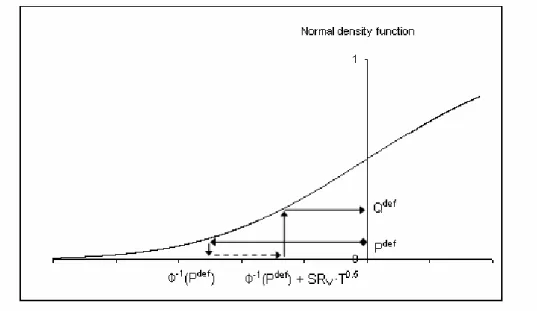
The company Sharpe ratio can simply be estimated based on actual and risk neutral default prob-abilities and the maturity. Second, it is quite robust to model changes. This will be discussed in the next subsections. A graphical illustration of the relationship between risk neutral and actual default probabilities, Sharpe ratio and maturity is given in figure 1.

Figure 1: Illustration of the relationship between actual and risk neutral default probabilities in the Merton framework. P Ddef: actual cumulative default probability, Qdef: risk neutral cumulative default probability, SRV: Sharpe ratio of the assets, T: maturity.

If we try to extract the market Sharpe ratio out of (4), we are faced with an additional problem: The Sharpe ratio of the assets µV−r

σV will usually differ from the market Sharpe ratio, since the

assets Vt will not necessarily be on the efficient frontier. The Sharpe ratio of the assets does not only capture the risk preference of investors, but also depends on the correlation of the assets with the market portfolio. The market Sharpe ratio can be calculated via a straight forward application of the CAPM:14 µV =r+ µM −r σM ·ρV,M ·σV ⇔ µM −r σM = µV −r σV · 1 ρV,M , (5)

whereρV,M denotes the correlation coefficient between the asset returns and the market returns.

Therefore, in addition to the Sharpe ratio of the assets, we will need an estimate of the corre-lation between the asset value and the market portfolio. At first, this correcorre-lation (ρV,M) seems to be a problem for practical applications, since it can neither be directly measured nor implic-itly inferred, e.g. from option prices. However, the correlation ρV,M can be approximated by the

14

correlation between the corresponding equity return and the market return (denotet byρE,M), i.e. by

ρV,M ≈ρE,M.

The error of this approximation is negligible, since - within the Merton framework - the equity value of a company equals a deep-in-the-money call option on the assets.15 For reasonable parameter choices, the approximation error is less than 3% (for rating grades above B) and 1% (for investment grade ratings) respectively (cf. Appendix A for details). Hence, the following approximation holds:

µM −r σM ≈ Φ −1_(Qdef_{(t, T))−Φ}−1_(Pdef_{(t, T))} √ T −t · 1 ρE,M .

Therefore, we define the Merton estimator for the market Sharpe ratio γ := µM−r

σM as: b γMerton:= Φ−1(Qdef(t, T))−Φ−1(Pdef(t, T)) √ T−t 1 ρE,M (6)

Please note, that we will need a sufficient sensitivity of the risk neutral default probabilityQdef(t, T) with respect to the Sharpe ratio for an empirical application. Otherwise noise in the data (e.g. bid-ask-spreads, inaccuracies in determining correlations and actual default probailities) will result in a very inaccurate estimation. That this sensitivity is large enough can be seen from the first derivative of (3) with respect to the Sharpe ratio:

∂Qdef_(T) ∂SRV = √1 2π ·e −1 2(SRV·T+Φ−1(Pdef(T))) 2 ·T. (7)

If we look, for example, at a BBB-rated obligor with a 5-year cumulative actual default probability of appr. 2.17%, the resulting model-based risk neutral default probability should be either 3.6% (for an asset Sharpe ratio of 10%) or 13% (for an asset Sharpe ratio of 40%) respectively (based on (3)). Assuming a recovery rate (RR) of 50% transforms this into a CDS spread of either 73 bp or 279 bp (cf. figure 2 for an illustration).16 This large difference indicates that noise in the input parameters will only have a minor effect on our Sharpe ratio estimation. The sensitivity with respect to noise in different input parameters is analyzed in more detail in section 3.

Although we have found a compelling result for an estimation of the market Sharpe ratio, the assumptions made under the Merton framework are subject to critisism.17 _{Therefore, we will relax}

the assumption about the default timing (cf. subsection 2.2) and the assumption about complete information (cf. subsection 2.3) in the following subsections by looking at more appropriate first passage time models.

Nevertheless, our estimator for the market Sharpe ratio contains a certain kind of robustness

15_{The option is deep-in-the-money, since annual default probabilities are less than 0.4% for investment grade}

companies and less than 10% for all obligors rated B and above. For deep-in-the-money options, gamma is appr. zero, i.e. we have an almost affine linear relationship between asset and equity value, cf. Hull (2005) for example.

16

Here we are using the approximation CDS-spread =λQ·(1-RR). The risk neutral default intensityλQis derived from the risk neutral cumulative default probability via the relationshipQdef_{(t, T) = 1−e}−λQ·(T−t)_.

17

Figure 2: Influence of the Sharpe ratio on the CDS spread in a Merton framework for different rating categories. Other Parameters: T=5.

against changes in the underlying assumptions: Since both default probabilities (Pdef _{and Q}def₎ are measured within the same model and substracted from each other, the effect of changes in the default modelling is - qualitatively spoken - reduced significantly.

2.2 Sharpe ratio estimation in a first passage time framework with obvservable asset values

Within the Merton framework, default can only occur at the maturity of the bond. This definitely poses a simplification of the real world. Therefore, we will analyze a first passage time framework in this subsection. In this framework default can also occur before maturity. We will show, that -although actual and risk neutral default probabilities are quite different from the Merton framework - our estimator for the Sharpe ratio is still accurate as long as the asset volatility is larger than 10%. In first passage time models a default occurs as soon as the asset value falls below a certain barrier.18 The asset value and the default barrier can both be either observable or unobservable. This subsection treats a model with a certain default barrier and observable asset values. A model with a certain default barrier and unobservable asset values based on Duffie/Lando (2001) is ana-lyzed in the next subsection.

As in the Merton framework, asset values Vt are assumed to follow a geometric Brownian mo-tion, default is modelled as the stopping time τ := inf{s > t;Vs ≤ L}, where L ∈ R denotes

the default threshold. In this framework, the cumulative real world default probabilityPdef(t, T)

18

Some authors use an even more general version of an ability-to-pay process, cf. Bluhm/Overbeck/Wagner (2003) for example.

betweent andT can be calculated as19 Pdef(t, T) = 1−P[ min t≤s≤TVs≥L] = Φ b−m(T −t) σ√T −t −e2σmb2 Φ b+m(T −t) σ√T −t (8) with b=ln(L Vt ); m=µ−1 2σ 2_{; σ=σ} V.

The default probability under the risk neutral measure Q can be calculated accordingly as

Qdef(t, T) = Φ bb−mb(T −t) σ√T −t ! −e2mbbb σ2 Φ b+m_b(T −t) σ√T−t (9) with bb=b=ln( L Vt ); m_b =r−1 2σ 2_{; σ =σ} V.

There is - in contrast to the Merton framework - no closed form solution for the Sharpe ratio µV−r

σV

in this model.

We now test the robustness of the simple Merton estimator for the Sharpe ratio and therefore introduce an adjustement factorAFF P by

SRM := µM −r σM =: Φ −1_(Qdef_(T)−Φ−1_Pdef_(T) √ T · 1 ρM,E ·AFF P =γMerton·AFF P, (10)

i.e. the adjustment factor shows, how far the estimate of the market Sharpe ratio via the standard Merton model deviates from the true market Sharpe ratio if a first passage model applies. Again, we have assumed thatρV,M =ρE,M, i.e. that the correlation between market and asset returns equals the correlation between market and equity returns. This equation holds for reasonable parame-ter choices in the first passage time framework as well, as we will be showing in the next subsection. The adjustment factor is dependent on the volatility, the Sharpe ratio and the credit quality (interpreted as actual default probability) of the company. We have numerically determined the adjustment factor in four steps: First, a combination of asset volatility, company Sharpe ratio, maturity and rating grade was choosen. We used r=5% as risk-free rate. Then, the ratio of asset value to default barrier (Vt/L) was determined based on (8) as to yield the cumulative actual de-fault probability of the rating grade choosen in the first step. Given Vt/L and the parameters set in the first step, the risk neutral default probability was determined via (9). In the fourth step, the actual and risk neutral default probability were plugged into the Sharpe ratio estimator and the difference to the Sharpe ratio set in the first step was determined. These four steps were repeated for all reasonable parameter choices. Details about the result can be found in Appendix B (table 7) and in the next subsection. Figure 3 plots the adjustment factor for a Sharpe ratio of 20% and a maturity of 5 years. The general shape is however also representative for other Sharpe ratios. The adjustment factor increases with decreasing credit quality and with increasing volatility, but for investment-grade titles and a volatility smaller than 10% the adjustment factor is close to 1.20

19_{Cf. Musiala/Rutkowski (1997).} 20

The boundary of 10% is of course dependent on the required accuracy. With a company Sharpe ratio of 20%, the adjustment factor equals 1.18 for an asset volatility of 10%, it is already 1.29 for an asset volatility of 7.5%. We will discuss this issue in a more general setting in the next subsection.

Asset volatilities below 10% usually only occur for financial-services companies, so this poses only a minor restriction.21

Figure 3: ’Credit quality smile’: Adjustment factor in the first passage time framework for different asset volatilities. Parameters: r=5%, SRA = 20%, maturity=5. Please note that the majority of traded bonds and CDS (by volume) has an investment grade rating.

The dependency on the asset volatility can be explained by the default timing: Fixing the cu-mulative default probability until time T, defaults will occur with a higher probability at the beginning of the period if the volatility is low.22 Since the difference between the risk neutral and the actual default probability increases with increasing maturity in the Merton model (cf. (3)), a large difference between the risk neutral and actual default probability can therefore only be explained by a large Sharpe ratio.23

We have shown in this subsection, that the Merton estimator for the Sharpe ratio derived in subsection 2.1 is still accurate in a first passage time framework as long as the asset volatility is larger than 10%. Asset volatilities below 10% are only reasonable for financial services companies,

21

In our sample of 125 companies of the CDS index CDX.NA.IG appr. 90% of all non-financial companies had an asset volatility of 10% or larger based on data from Moody’s KMV. In contrast, for financial services companies, the volatility is 10% or smaller in appr. 75% of all cases.

22

I.e. the conditional expected default timeE[τ|τ < T ] conditional on default untilT is lower for lower asset volatilities if we only compare stopping times τ withP[τ < T] =c. Please note that - all other parameters being equal - the default probability declines with declining asset volatility. Therefore, the expected value of the default time will also decrease. In this case, comparing only stopping times with a fixed cumulative default probability simply means, that the declining asset volatility is always balanced by a lower t0-asset-value.

23_{A possible way to increase the accuracy of our estimation could be a substitution of the maturity by the expected}

default time conditional on default up to time T. This expected default time could be derived from the cumulative default probabilities for each rating grade, see table 11 in Appendix D.

so the Merton estimator is still accurate for all non-financial services companies. Although actual and risk neutral default probabilities both differ from the Merton model, the difference between (the inverse cumulative normal distribution of the) actual and risk neutral default probability is merely affected.

2.3 Sharpe ratio estimation in a first passage time framework withunobvservable asset values

Credit spreads predicted by simple first passage time models are not able to fully predict the credit spreads that can be observed on the markets.24 In particular, for short term maturities market credit spreads (or risk neutral default probabilities respectively) are higher than a simple first pas-sage time model would suggest.

In this subsection, we analyze a model - proposed by Duffie/Lando (2001) - which is able to explain the credit spreads observed in the markets. We show, that the simple Merton estimator is still accurate in this setting for all investment grade entities. First, we will explain the reasons for choosing the Duffie/Lando framework. Then we will analyze the robustness of the Merton estimator in this setting.

Higher credit spreads for short term maturitites seem to be mainly attributable to credit risk and are unlikely to be mainly due to liquidity effects, other risk factors or market imperfections.25 This justifies the explanation of these higher credit spreads within credit risk models. Most impor-tantly, the literature points out that asset values may be unobservable due to imperfect information structures.26 Therefore, the current asset value becomes a random variable, which in turn has the effect of increasing short term default probabilities. A model with unobservable asset values has been developed by Duffie/Lando (2001). In addition, the default barrier may be unobservable itself. This is consistent with the fact that the recovery rate is usually assumed to be a random variable rather than a fixed value.27 An unobservable default barrier leads to a significant increase in the short term default probability. Long term default probabilities are, however, less affected, since the asset volatility dominates uncertainty for longer time periods. A model with an unobservable default barrier has been implemented by Finger et.al. (2002) within the commercial model Cred-itGrades. Finally, asset values may not be lognormally distributed and may incorporate jumps. This increases the short term probability, that the asset value will fall below the default barrier.28 A model with jumps in the asset value process has been analyzed by Zhou (1997).

In this subsection, we will focus on the model of Duffie/Lando (2001). We choose the Duffie/Lando model for our analysis as it is the only structural model consistent with reduced form credit pricing. Reduced form credit pricing is currently the major approach for pricing credit

deriva-24_{Cf. Duffie/Lando (2001), Duffie/Singleton (2003) and Sch¨onbucher (2003) for a detailed discussion.} 25

Cf. for example Sch¨onbucher (2003).

26_{Cf. Duffie/Lando (2001).} 27

Cf. for example Moody’s (2007). A random recovery rate could though also be induced by introducing random insolvency costs, i.e. costs incurred at default due to direct insolvency expenses, losses in asset value due to a forced sale in an insolvency process and revaluation of assets serving a specific purpose for the respective company.

28

Note that for long term maturities, a higher volatility has the same effect as adding jumps to the process. Therefore long term default probabilities will not be affected in the same manner than short term default probabilities.

tives.29 Reduced form pricing models use default intensity processes to derive credit spreads. The Duffie/Lando model is the only structural model so far that yields a default intensity.30 In addition, the Duffie/Lando model incorporates a sophisticated structural model of default (i.e. a strategic setting of the default barrier based on the asset value process, tax shield and insolvency costs) and - given an appropriate calibration - results in realistic default intensities for short and long term maturities.

We will show that - although the default probabilities implied by this model differ substantially from the classical Merton model - thedifference between risk neutral and actual default probabili-ties is almost the same as in the Merton model as long as the asset volatility is above 10%. We are then able to show that the simple Merton estimator for the market Sharpe ratio (6) is accurate in the Duffie/Lando-framework for investment grade companies and asset volatilities above 10%. In the Duffie/Lando framework the asset value is modelled as a geometric Brownian motion with initial value z0 :=ln(V0), volatilityσ and drift mP := µ−δ (actual drift) and mQ := r−δ (risk

neutral drift) respectively, where δ denotes the constant payout rate. Like in the classical first passage time framework, default is modelled as the stopping time τ := inf{s > t;Vs ≤L}, where

L ∈ _R denotes the default threshold. In contrast to the classical first passage time framework, investors are not able to observe the asset process directly. Instead they receive imperfect infor-mation Y(ti) := ln

c

Vti

= ln(Vti) +αUti at the times ti,1 ≤ i ≤ n, where U(ti) is normally

distributed and independent of Bti and α is a parameter specifying the degree of noise in the

in-formation received by the bond/CDS investors. Therefore, the inin-formation filtration given to the bond/CDS investors is31 H_t=σ({Y(ti), ..., Y(Tn),1τ≤s: 0≤s≤t}). As in Duffie/Lando, we will focus on the case, where investors receives simply one noisy information about the asset value. Under these assumptions the conditional densityg(x|Yt, z0, t) of the asset value Vt conditional on the noisy information Yti and survival up to timet can be explicitly calculated (cf. Duffie/Lando

(2001) for details).

The calculation of the cumulative default probabilities requires a weighted application of (8) over all possible asset values Vt, where the weight is - roughly speaking - the probability of the asset valueVt32, i.e. Pdef(t, T) = Z ∞ L P_{F P}def(t, T, x) | {z }

PD(first passage time) if Vt= x

g(x|Yt, z0, t)

| {z }

Prob.,that Vt= x

dx, (11)

where P_{F P}def(t, T, x) denotes the probability that an asset value process starting in tatVt=x will fall below the default barrier up to time T (cf. (8)) and g is the conditional density of the asset value at t given the filtration H_t. Formula (11) can be used to calculate both the actual and the

29_{Cf. Sch¨onbucher (2003).} 30

Defaults in a Merton framework cannot be described by default intensity processes, since the probability of a default from t(today) until t+δtis always zero or one for a sufficient smallδt. A default intensity does also not exist in the Zhou (1997) framework, since the default time cannot be represented by a totally inaccessible stopping time (which is a consequence of the fact, that the default barrier may be hit/crossed by the normal diffusion process with positive probability) (cf. Duffie/Lando (2001) for details).

31

Of course, all investors can obvserve whether a default has already occured.

32_{Of course the probability of a single valueV}

twill be zero for non-degenerated parameter choices, since we operate

risk neutral default probability.

As in subsection 2.2, we now test the robustness of the Merton model estimator, i.e. we again define an adjustment factorAFDL by

µM−r

σM

=γM erton·AFDL. (12)

This adjustment factor may depend on all parameters included in the model, which we will group into two different classes: Class 1 captures all parameters that can easily be observed in the mar-ket, i.e. the actual default probability (which is actually a combined parameter of all other input parameters) and the maturity. Class 2 captures all parameters that cannot be easily observed in the market, i.e. the asset volatility σ, the payout rate δ or the risk neutral net asset growth rate

m := r−δ, the starting point of the asset value process in t= 0 (Z0), the default barrier L, the

noisy asset value observed att (Vb_t) and the accounting noise α. If the adjustment factor depends

on any class-2-parameter, this will affect our ability to correctly measure the market Sharpe ratio, since these parameters will possibly be subject to significant calibration errors.

We have evaluated (12) for all reasonable combinations of input parameters.33 _{The calculation}

was carried out in four steps: In the first step, a combination of a specific rating grade and all parameters from the Duffie/Lando framework excluding the asset value Vt was choosen. Please note, that this also involves the specification of the asset Sharpe ratio in order to determine the real world drift of the asset value process. Then, based on (11), the asset value Vt was numerically determined as to result in the cumulative actual default probability for the respective rating cate-gory. Given the asset valueVtand the other parameters choosen in the first step, a straight forward application of (11) based on risk neutral parameters was used to determine the risk neutral default probability. In the fourth step, the Merton estimator was calcualted based on these model-based actual and risk neutral default probabilities. Comparison with the Sharpe ratio specified in step 1 yields the adjustment factor. These four steps were repeated for all reasonable parameter com-binations. Detailed results can be found in Appendix Appendix B. The minimum and maximum adjustment factor of all parameter combinations are also plottet in figure 4 as a function of the rating grade.

The main results can be summarized as follows: First, the adjustment factor is close to 1 for all parameter combinations as long as the asset volatility is below 10%34 and the resulting actual

33

Input parameters used were: σ: 3%−30% (the 5% and 95% quantile for the asset volatility from KMV was 6% and 25% respectively), Sharpe ratio of the ability-to-pay process: 10% to 40% (The market Sharpe ratio is usually assumed to be anywhere between 20% and 50%, due to a correlation of lower than 1, the asset Sharpe ratio should be smaller),m: 0%−5% (m <0 would imply, that the payout rate is larger than the risk free rate, m=5% was choosen as an upper limit to reflect (almost) zero payout at a risk free interest rate of 5%.),α: 0%−30% (α= 0% reflects the classical first passage model with observable asset values, Duffie/Lando use 10% as a standard value, the upper limit of 30% is also based on Duffie/Lando(2001)),Vbt=Z0andVB for all combination that resulted in rating grades

from AA to B. The caseVbt> Z0andVbt< Z0 was also analyzed, the results merely differ from the caseVbt=Z0and

are available upon request. Please note, that the result is continuous with respect to all input parameters. Therefore a numerical approximation on a certain grid is feasible.

34_{The boundary is of course dependent on the required accuracy. The adjustment factor is higher if asset value}

uncertainty is lower (cf. tables 7 and 8 in Appendix B). Even in the case of observable asset values, the adjustment factor is on average smaller or equal to 1.12. For likely parameter combinations, the error is smaller than 10% for asset volatilities larger than 10% (cf. Appendix B).

default probability belongs to an investment grade rating (cf. figure 4). This can be explained by looking at the impact of the parameters introduced in the Duffie/Lando framework: All of them do effect the actual default probability as well as the risk neutral default probability in the same direction, e.g. increasing the information uncertainty increases the actual as well as the risk neutral default probability. The Sharpe ratio is the only parameter that solely has an effect on the actual default probability. This explains qualitatively, why the adjustment factor is close to one in most cases. Second, the adjustment factor can be accurately determined simply based on knowledge of the class-1-parameters and the actual default probability as long asσ > 10%. For any given com-bination of default probability and maturity, parameters that cannot be observed easily (e.g. asset volatility, default barrier, asset value or accounting noise) do not significantly affect the adjustment factor.

Please note the special role of the actual default probability: For example, an adjustment fac-tor of appr. 1.7 (i.e. significantly above 1) occurs for an asset value of Vt = 108, default barrier

L = 100, σ = 10%, T = 5, SR = 40% and α = 0%. If this were due to any class-2-parameter, empirical applications would be hardly possible due to calibration errors of class-2-parameters. But as soon as we change anyof these parameters so that the resulting actual default probability belongs to an investment grade rating (e.g. increasing Vt, decreasing α, decreasing σ (up to a level of 10%)), the adjustment factor will be close to 1. Any combination of these parameters that yields a given actual default probability also yields (almost) the same adjustment factor. All in all, class-2-parameters may have an influence on the adjustment factor. This influence can, however, (almost fully) be captured by the rating smile.

If we examine the influence of certain parameters in more detail, we can observe the following: First, the adjustment factor decreases with increasing asset value uncertainty (α). This means, that the Merton estimator overestimates the Sharpe ratio for high asset value uncertainty. I.e., a higher asset value level uncertainty increases the risk neutral default probability. The effect is quite interesting: All other parameters being equal, a high risk neutral default probability can either be explained by a higher risk aversion or by a higher asset value uncertainty. The effect is more pro-nounced for higher rating grades. We think, this could explain at least part of the perceived high credit spreads for high rated obligors.35 This dependency on the asset value uncertainty is due to the difference between the asset value estimation int under the risk neutral compared to the real world probability measure. Given unbiased information, the asset value intunder the risk neutral probability measure equals the asset value under the real world probability measure. Assume now, that we only have information about the asset value int= 0 and we have observed, that no default has occured up to t. In this scenario, the best estimate of the asset value intwill be lower under the risk neutral probability measure due to the lower drift of the assets in the risk neutral world. This lower asset value will result in a higher risk neutral default probability estimate from ttoT. The higher the noise in the information about the asset value int, the more will the information about survival influence our estimate of the asset value. Second, the parameter combinations leading to the minimal and maximal adjustment factor in figure 4 belong to ’unlikely’ parameter combina-tions. Table 7 in the Appendix shows the dependeny of the adjustment factor for a maturity of 5

35

E.g. Huang/Huang (2005) show, that only appr. 20% of the spread for high rated obligors can be explained by traditional asset value models compared to up to 100% for lower rated obligors. Cf. also Hull et.al (2005) for a discussion.

years and a Baa-rating36 for α = 0% and s = 0, e.g. for the extreme of observable asset values, table 8 for α = 30% and s= 3 representing large uncertainty about the asset value. The absolut maximum is reached for small asset volatilites, no uncertainty and a high risk neutral asset growth rate (i.e. a low payout rate). One would expect small asset volatilities to be linked with ’value firms’ whereas low payout rates usually apply to ’growth companies’. The absolut minimum is reached for small asset volatilities and high payout rates (i.e. a low risk neutral asset growth rate m), which would suit the usual assumptions about value firms, but for a high uncertainty about the current asset value, which one would usually assume for growth companies. Depicting values which one would usually assume for value firms and growth firms, we can see that the adjustment factor will be even closer around the mean value.

Third, the (average) adjustment factor increases with decreasing credit quality. This also simply states that the classical Merton model overestimates risk neutral default probabilities for low rated obligors. Therefore, the adjustment factor is larger than one. This again has the effect, that if sim-ple models like the Merton model are applied, the spread difference between high quality obligors and low quality obligors will seem to be too low.

Figure 4: Adjustment factor in the Duffie/Lando model for different rating grades. The minimum and maximum is taken over the parameters 10% ≤ σ ≤ 30%, 0 ≤ α ≤ 30%, 0 ≤ m ≤ 5%, 10%≤SRV ≤40%, 0≤s≤3. Other parameter: T=5.

All in all, we have shown in this subsection, that the simple Merton estimator for the Sharpe ratio is still valid in the Duffie/Lando (2001) framework for investment grade entities as long as the asset volatility is larger than 10%. Investment grade bonds/CDS constitute the majority of traded bond/CDS volume. Asset volatilities smaller than 10% usually only occur for financial services companies - cf. subsection 2.2 - so this is just a minor restriction.

36_{We choose this as an example, since 5-year CDS are the most liquid ones usually used in empirical studies, cf. for}

3

Empirical analysis

3.1 Data sources and descriptive statistics

Our data sample consists of 125 North American companies based on the Dow Jones CDX.NA.IG-index, which is an investment grade CDS index published by markit and a consortium of 16 in-vestment banks.37 _{We used 5-year CDS spreads to derive risk neutral default probabilities. EDFs}

(expected default probabilities) from Moody’s KMV data base were used as a proxy for the actual default probabilities and correlations with the S&P500-index as a proxy for the correlations with the market portfolio. In some occasions, Moody’s ratings were used in addition for the actual default probability. All data was taken from the period from January 2003 until June 2007. Credit Default Swaps are OTC credit derivatives that have become widely popular over the last years with growth rates of over 100% (nominal value) in 2005 and 200638. Their main mechanism is quite simple: The protection buyer periodically pays a predefined premium (usually quarterly) to the protection seller. In case of a credit event, the protection seller has to cover the losses incurred on a predefined reference obligation, i.e. he he has to pay an amount equal to the difference between the nominal and the current market value of the predefined reference obligation to the protection buyer. As usual, put into practice, things turn out to be more complicated: The credit event has to be precisely defined, a basket of reference obligations has to be specified39and the term ’market value’ at the time of default has to be clearly specified. As in most academic research, we will assume, that the extent of these specification does not have a significant value and therefore CDS can be prized as if these implicit options were not part of the game.40

The 5-year CDS spreads (bid/ask/mid) used in our analysis were taken from Datastream. Only dates with at least one trade for the respective CDS were used to avoid potential errors from pure market maker data. We used CDS mid spreads for our analysis. Bid/ask-spreads served for con-sistency checks and sensitivity analysis. The risk neutral default intensity λQ was derived by the approximation s= λQ·LGDQ out of the CDS spread s and the risk neutral LGD41. A recovery rate of 50% was used.42

37_{The data is based on the CDX.NA.IG.8-index. By first fixing the constituents list and then analyzing historical}

data of these constituents, our data may be subject to a selection bias, since all these companies have performed well enough to be included in an investment grade index. We are however not interested in the performance of the index or any of its constituents but only examine risk pricing based on risk neutral and actual default probabilities.

38

Total outstanding market volume was $26 trillion at the end of 2006 concerning to the ISDA, growth rates in 2005 and 2006 were 103% and 101% respectively (cf. ISDA 2006 year-end market survey).

39

Defining only a single reference obligation is not possible for practical reasons, which usually leads to a ’cheapest-to-deliver’ option for the protection buyer, who can normally choose which reference obligation to sell to the protection seller in case of a default.

40_{Cf. Berndt et.al. (2005) for example.} 41

The simple equations=λQ·LGDQis only valid if the LGD is given as a fraction of market value. In case of a

recovery/loss given as a percentage of face value - as it will usually be the case when using rating agency data - default intensity and recovery enter the pricing formula asymmetrically. For practical pruposes, the differences are minimal. Cf. Duffie/Lando (1999) and Duffie/Lando (2003) for discussion. Cf. also Duffie/Singleton (2003) or Sch¨onbucher (2003).

42_{Based on Moody’s (2007) the average default rate from 1982-2006 was 38% (value-weighted basis) and 46% (same}

weight for all years) respectively for senior unsecured bonds. The interquartile range based on yearly averages from 1982-2006 is 39%-54% on a 1-year basis and 43% to 51% on a 5-year basis. Other studies also derive recovery rates of approximately 50%, e.g. Altman/Kishore (1996) (48%) and Carty/Liebermann (1996) (54%). As we are mainly interested in an upper limit for the Sharpe ratio estimation, we choose a recovery rate of 50%, therefore slightly above

Variable N Mean Median Coeff of Variation 25th Pctl 75th Pctl CDS mid in bp 19945 51.2 41.77 74.74 28.1 62.5 CDS offer in bp 19945 53.1 43.63 72.73 30.0 64.0 CDS bid in bp 19945 49.4 40 76.96 26.3 60.5 ∆(offer, bid) in bp 19945 3.8 3.62 54.22 2.7 4.7 Asset Vol. 19945 15% 15% 38.07 11% 18% EDF1 19945 0.2% 0.1% 174.12 0.05% 0.15% EDF5 19945 1.93% 1.38% 95.45 1.00% 2.15% Moody’s PD1 14743 0.15% 0.10% 120.22 0.05% 0.18% Moody’s PD5 14743 2.01% 1.63% 75.12 0.93% 2.51% ∆(EDF1, Moody’s PD1) 14743 0.00% -0.01% 11660.05 -0.11% 0.06% Correlation 19945 0.51 0.52 24.53 0.42 0.60

Table 2: Descriptive statistics for main input parameters. EDF1/EDF5/Moody’s PD1/Moody’s PD5 denote the respective 1- and 5-year cumulative default probabilities.

Expected default frequencies (EDFs) from Moody’s KMV data base were used as a proxy for the actual default probabilities. EDFs are default probabilities, which are based on a Merton-style structural framework.43 The calibration is, however, done more pragmatically based on a large set of historical data and on discriminant analysis. EDFs are widely used in the banking industry and also constitute a part of some of the internal rating systems of large banks. We used 1-year EDFs and derived multi-year EDFs by Moody’s cumulative default probabilites per rating grade.44 The main advantage of EDFs compared to other ratings for our purpose is its link to market data: The current asset volatility and equity value are direct input parameters, therefore EDFs constitute a ’point-in-time’ estimation of the current default probability. In contrast to EDFs, the ratings of the large rating agencies are normally defined as ’throughthecycle’ratings, which in effect -results in different default probabilities for a specific rating grade dependent on the current overall economic outlook. In some circumstances, Moody’s ratings were used, if so, they were taken from Bloomberg. The ratings were mapped to default probabilities via a logarithmic approach based on raw data from Moody’s (2007), i.e. ln(P D) =β1+β2∗N RG, where NRG denotes the numerical

rating grade ranging from 1 (Aaa) to 16 (Baa3).45

Finally, we used 3-year weeekly46 correlations of the reference entities share price returns with the S&P-500 index. The share prices were taken from Datastream. Companies without a NYSE or NASDAQ listing were removed from the sample. A floor of 20% was applied to the estimation of correlations.

Our final data set consists of 19,945 date/company-combinations for which CDS spreads, EDFs and correlations were available. Table 2 gives an overview of these main input parameters.

the average indicated by the studies cited above. Lower recovery rates result in lower risk neutral default probabilities and therefore in lower Sharpe ratio estimates.

43

Cf. for example Moody’s KMV (2007).

44_{Cf. Appendix D for details.} 45

The log-approach is a common approach for the calibration of default probabilities (cf. for example Bluhm et.al (2003)). The resulting table of cumulative default probabilities can be found in Appendix D.

46_{The calibration of correlations has a minor effect on the overall result, using 2-year or 1-year correlation did not}

Variable N Mean Median Coeff of Variation 25th Pctl 75th Pctl

λQ_/λP _{(EDF) 19945 3.38 2.74 71.36 1.87 4.12}

λQ_/λP _{(Moody’s) 14743 3.40 2.55 87.09 1.70 4.03}

Sharpe ratio market (EDF) 19945 42.46% 37.23% 76.33 21.91% 56.80%

Sharpe ratio company (EDF) 19945 19.56% 19.04% 60.32 11.76% 26.71%

Sharpe ratio market (Moody’s) 14743 39.01% 35.25% 75.70 21.50% 53.03%

Sharpe ratio company (Moody’s) 14743 18.70% 17.79% 67.63 10.15% 26.51%

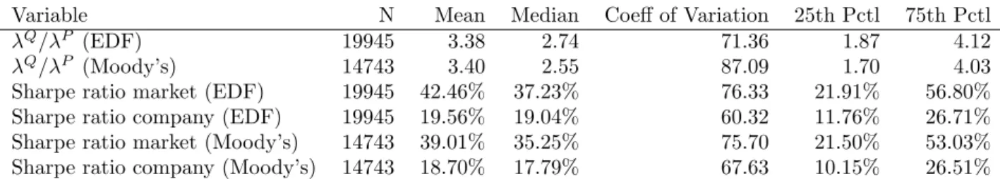
Table 3: Descriptive statistics for main output parameters. (EDF) and (Moody’s) denotes, that the respective parameter was calculated via EDFs and default probabilities derived from Moody’s respectively. SR: Sharpe ratio. λQ andλP denote the actual/risk neutral default intensities.

3.2 Empirical findings and discussion

Based on the data described in subsection 3.1 and the Merton estimator for the Sharpe ratio derived in section 3.1, we estimate the implicit company and market Sharpe ratios for each of the 19,945 observations.

3.2.1 Results of Sharpe ratio estimation

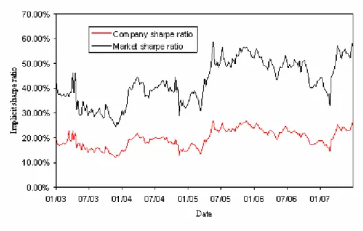
Our estimation yields an average market Sharpe ratio of 42%, with an average company Sharpe ratio of 20% and an average correlation of 0.51 (cf. table 3). The median market Sharpe ratio is 37%. Half of the observations result in a company Sharpe ratio between 12% and 27% (market Sharpe ratio: 22% and 57%).47 Using actual default probabilities from Moody’s leads to similar, though slightly smaller estimates for the average company Sharpe ratio (19%) and market Sharpe ratio (39%). Figure 5 shows, that the implicit market Sharpe ratio fluctuates in a range between 30% and 50% over the period 2003 to 2007 with peaks in mid 2005 (downgrades of Ford and General Motors) and mid 2007 (subprime crises). The volatility of the market Sharpe ratio is appr. 50%. The disaggregation with respect to sectors shows a quite homogenous result. Seven out of eight sectors have average implicit market Sharpe ratios between 30% and 45% as can be seen in table 4 The only outlier is the consumer stable sector with an average implicit market Sharpe ratio of 67%. This is due to a lower correlation of this sector with the market portfolio. Other studies have pointed out the fact that correlations are not stable over time and seem to increase in adverse market environments.48 _{Such adverse market environments are especially important when looking}

at credit valuations, since only the tails of the distribution matter in this case. This may explain the high implicit Sharpe ratios estimated for this sector. The lower Sharpe ratio estimates for financial services companies may be explained by their low asset volatility. The average asset volatility of a financial service company based on Moody’s KMv data is 8.8%. The financial services sector is the only sector which has an asset volatility smaller than 10%. Asset volatilites below 10% imply higher adjustment factors (cf. section 2.3), i.e. the Merton estimator underestimates the true Sharpe ratio.

47

This interquartile range may seem large at first. We do though want to point out, that our estimation was conducted on a single-obligor/single-date level. We are not aware of any authors, that have reported the results for dividend/earnings-discount models on this level, usually only aggregated data is provided. Based on own calculations, we would though expect these estimations to have at least equal variations.

Figure 5: Implicit Sharpe ratio based on CDS spreads and EDFs as a function of time.

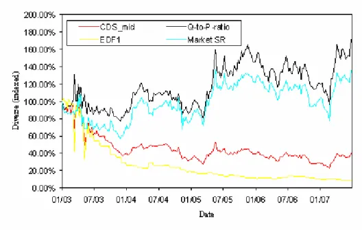
Some studies have used the ratio of risk neutral to actual default probabilities (’Q-to-P-ratio’) as a measure for risk aversion of investors.49 We would like to point out a major difference of the Q-to-P-ratio compared to our Sharpe ratio estimator. Whereas the Sharpe ratio over the time period under consideration has only slightly increased, the increase in the Q-to-P-ratio was much stronger (cf. figure 6). This is a direct effect of the increasing credit quality in the sample period (cf. section 2.3). From a theoretical point of view, the Sharpe ratio seems to be a much better indicator for risk aversion.

3.2.2 Portion of CDS spread attributable to credit risk

Some authors have argued, that especially for higher rating grades a significant part of the credit spread is not due to credit risk.50 Therefore we have analyzed our Sharpe ratio estimates sepa-rately for each rating grade. In theory, it should be independent of the credit quality. Based on the adjustment factors derived in section 2.3 slight variations may,, however be plausible. Table 5 compares the minimum and maximum of plausible Sharpe ratio estimates based on the adjustment factors derived in section 2.3 to our actual estimates. We can indeed see that our Sharpe ratio estimates for higher rating grades seem to be too high compared to the estimates for lower rating grades. In fact, testing the null-hypothesis that the mean Sharpe ratio for the high rating grades Aa and A equals the mean Sharpe ratio for the rating grade Baa results in p-values below 1%, e.g.

49

Cf. for example Berndt et.al. (2005), Amato (2005) and Hull et.al. (2005).

50

Sector N (d/c) N (c) SR company (EDF) Correlation SR market (EDF)

Communications and Technology 2,401 13 20.92%** 0.53 44.61%

Consumer Cyclical 4,653 25 20.72%** 0.51 43.71%* Consumer Stable 2,291 14 23.15%** 0.40 67.33%** Energy 1,340 6 17.50%** 0.43 42.95% Financial 3,358 18 16.32%** 0.54 33.21%** Industrial 2,659 14 19.20% 0.56 36.17%** Materials 1,947 9 22.91%** 0.59 40.23%** Utilities 1,296 6 12.75%** 0.45 29.76%** Average 19,945 105 19.56% 0.51 42.46%

Table 4: Sharpe ratio estimator for different industry sectors. N (d/c): Number of company/date combinations available for this sector; N (c): Number of companies in this sector with at least one observation. */** denotes that the difference to the total average is significant at the 5%/1% confidence level.

Rating grade Merton es-timator min (SR = 20%) Merton esti-mator max (SR = 20%) Merton es-timator min (SR = 30%) Merton esti-mator max (SR = 30%) Actual Merton estimator Aa 17.57% 23.45% 26.35% 35.18% 28.90%** A 16.83% 23.30% 25.25% 34.95% 22.98%** Baa 15.77% 23.03% 23.65% 34.55% 17.97% Ba 14.18% 22.43% 21.27% 33.64% B 11.63% 20.21% 17.44% 30.32%

Table 5: Company Sharpe ratio estimator for different rating grades. Merton estimator min/max: Minimum/Maximum model-based Merton estimator after adjusting for the adjustment factors de-rived in subsection 2.3 if the company Sharpe ratio is 20%/30%. AF: adjustment factor, SR: company Sharpe ratio. P-Value: H0 : mean Sharpe ratio for the rating grades Aa and A equals

the mean Sharpe ratio of the rating grade Baa (17.97%). */** denotes that the difference to the average Sharpe ratio in rating grade Baa (e.g. 17.97%) is significant at the 5%/1% confidence level.

the difference is largely significant.51

If we look at a hypothetical change in the CDS spreads, that would make it a ’fair’ game - e.g. that would yield the same Sharpe ratio for a all rating grades - we find that the spread of an Aa-rated obligor has to decline by appr. 50% to yield the same Sharpe ratio than for an average Baa-rated obligor. Given an average spread of 32 bp for an Aa-rated obligor, this means a reduction of 16 bp. We do however have to point out, that less than 1% of all obligors are rated Aa in our sample which could be a source of inaccuracy. The spread of an A-rated obligor has to decline by appr. 30% to yield the same Sharpe ratio than for an average Baa-rated obligor. Given an average spread of 37 bp for an A-rated obligor, this implies a reduction of 12 bp. Alternatively, the spread of an A-rated obligor has to increase by 20% or 7 bp to match the Sharpe ratio of an average Aa-rated obligor. The spread of a Baa-rated obligor has to increase by appr. 50% (29 bp) or 20% (10 bp) to yield the same Sharpe ratio than for an average Aa- or A-rated obligor.

Summing up, even in an unobservable asset value framework credit spreads for high quality

com-51

Figure 6: Development of 5 year CDS spread, 1-year EDF, implicit market Sharpe ratio and Q-to-P-ratio as a function of time.

panies still seem to be too high compared to credit spreads for lower quality companies.52 This result is in line with other empirical research, which has stressed the role of taxes, transaction costs, liquidity and other parameters absent in a perfect market setting.53 Although most of the research focuses on bond pricing, an effect on CDS spreads seems to be be likely as well based on arbitrage arguments. It is not the scope of this paper to quantitatively evaluate these effects. We do only want to stress, that all these effects will lead to a decrease in the implicit Sharpe ratio, since they result in a declining portion of the CDS spread attributable to credit risk.54 Therefore the derived market Sharpe ratio of 42% (mean) and 37% (median) is still valid as an upper limit on the market Sharpe ratio in these settings.

52_{One could argue, that higher quality companies have less idiosyncratic risk than low quality companies, which}

could justify the observed differences in Sharpe ratio estimations. The behavior of the correlation with respect to rating classes is quite akward in this sample. The correlation is a increasing function of the EDF-measure and a decreasing function of the default probability derived from Moody’s rating. Companies with a high correlation with the market seem to have predominantly high Moody’s ratings and high EDFs, whereas the opposite seems to be true for companies with a low correlation. We do not aim to resolve this conflict in this paper and leave this question for further analysis.

53_{Cf. Huang/Huang (2005) and Liu et.al. (2007).} 54

The tax rate plays a special role, since - in contrast to other effects - it does not only have an influence on the portion of the credit spread attributable to credit risk but can also have an effect on the volatility as it may in theory - dependent on the tax system - decrease the volatility of the after tax cash flow. It is however hardly imaginable that CDS spreads will increase, if taxes are lowered. Therefore the general statements will - under realistic assumptions - hold true for tax effects, too. For a detailed discussion on the effect of capital income taxes on asset prices cf. for example Rapp/Schwetzler (2006).

3.2.3 Adjustment for tax effects

In the next step, we have adjusted our estimator for the different tax treatment on equity and debt markets. Looking at equity returns, the capital gains should usually be tax free and only the dividend part of the return is reduced by tax payments. In contrast, capital gains do - on average - not pose a significant part of credit returns, as bonds are normally issued at par. The interest received on the bonds is normally subject to full tax payments. Since CDS are often held by banks, we have applied a different method to extract the tax effect out of CDS spreads:55 Thinking in a P&L logic (and ignoring operative expenses), the difference between the CDS spread (income) and the expected loss (as expected payout rate to the protection buyer) is - on average - taxable on corporate level. Therefore, the after tax cash flow received by an investor equals (CDS spread − expected loss)·(1−corporate tax rate). Using a corporate tax rate of 35% yields an average company Sharpe ratio of 15% and a market Sharpe ratio of 32%.

3.2.4 Sensitivity with respect to noise in input parameters

In section 2, we have shown, that the results are quite robust to model changes. Besides misspec-ifying the model, noise in the input parameters pose another possible source of inaccuracy. We therefore tested the sensitivity of our results with respect to the main input parameters. The results are shown in table 6. Changes of 10% relative to its original value result in a market Sharpe ratio of appr. 5% higher/lower for all analyzed parameters (EDF: actual default probability, CDS spread, recovery rate, correlations). We would like to focus on two parameters: First, the sensitivity with respect to the CDS spread and second, the sensitivity with respect to the recovery rate.

The sensitivity with respect to the CDS spread can be used, if there is evidence that only a portion of the CDS spread is attributable to credit risk. For example, if only 90% of the CDS mid spread were attributable to credit risk, this would decrease our estimation for the market Sharpe ratio by 4.6% (from 42.5% to 37.9%). In particular extracting the part due to liquidity risk may increase the accuracy of our estimation.

We expect the recovery rate modelling to be another focus of further research. Based on Moody’s (2007), the recovery rate volatility is significantly smaller than the default rate volatility, with a coefficient of variation of appr. 25% on a 1-year basis compared to a appr. 60% for the default probability. The interquartile range is 39%-54% on a 1-year basis and 43%-51% on a 5-year ba-sis. Research on the recovery rates has soared over the last years, indicating, that recovery rates vary by industry sector and through the business cycle. E.g., Moody’s (2007) indicates a signif-icant negative correlation between realized recovery rate and realized default rate. It remains to be shown, if this relationship holds true for expected values as well. Different recovery rates for specific sectors/companies may also explain some of the differences between the implicit Sharpe ratios measured.

55

Company Sharpe ratio Market Sharpe ratio Market Sharpe ratio (at) Base Case 19.56% 42.46% 32.13% CDS spread -10% 17.40% 37.90% 28.56% CDS spread +10% 21.55% 46.66% 35.46% RR +10% 21.76% 47.11% 35.81% RR -10% 17.60% 38.33% 28.89% EDF -10% 21.44% 46.41% 35.32% EDF +10% 17.83% 38.84% 29.25% Correlation +10% 19.56% 38.60% 29.21% Correlation -10% 19.56% 47.18% 35.70%

Table 6: Sensitivities of Sharpe ratio estimation for the main input parameters. Sharpe ratio market (at) denotes the estimation for the market Sharpe ratio after tax adjustment. RR: recovery rate, EDF: expected default frequency.

3.2.5 Comparison to other equity premium estimates

These findings strongly support current research on the equity premium, which has averaged appr. 7-9% over the last 50 years.56 _{This is equivalent to a Sharpe ratio of appr. 40-50%. Current}

research suggests, that the development of stock markets over the last 50 years was partially driven by extraordinary gains and cannot be explained by fundamentals alone.57 A ’fair’ equity premium is seen at appr. 3-5% in most academic research, equivalent to a Sharpe ratio of appr. 15%-30%58_.

Taking our Sharpe ratio estimate of 42% and 32% (after tax adjustment) and taking into account, that only part of the total credit spread is attributable to credit risk yields the same qualitative result: Sharpe ratios of above 40% simply do not seem to be priced in current asset values.

4

Conclusion

In this paper, we have introduced a new framework for estimating the equity premium. We measure the risk attitude of investors based on credit valuations and transforms it to an equity premium via structural models. This approach offers a new line of thought for estimating the equity premium that is not directly linked to current methods. In addition, our approach is suited to link the cur-rent literature about credit risk premia on the one hand and the equity premium on the other hand. First, we have theoretically analyzed the estimation of Sharpe ratios out of credit valuations based on a simple Merton model and a more advanced structural model of default by Duffie/Lando (2001) including unobservable asset values. Based on the Merton model, we have developed a simple es-timator for the market Sharpe ratio. This eses-timator only uses actual and risk neutral default probabilities, the maturity and equity correlations. We do neither have to calibrate a structural model nor do we have to estimate earnings or dividend growth. The theoretical results show an astonishing robustness of this simple estimator with respect to model changes. Although actual and

56

Cf. for historical equity premia Ibbotson (2006) and for an overview and discussion Fama/French (2002), Claus/Thomas (2002) and Illmanen (2002).

57

Among others, Fama/French (2001) derive an implicit Sharpe ratio for the U.S.-market from 1951-2000 of 15% based on the dividend growth model and a Sharpe ratio of 25% based on the earnings growth model. Claus/Thomas (2001) derive an equity premium of 3.4% based on an Earnings forecast model, which equals a Sharpe ratio of appr. 17%-23% (based on a market volatility of 15%-20%).

58