Variance risk premia for agricultural commodities

Economics Publications Economics

2019

Variance risk premia for agricultural commodities

Variance risk premia for agricultural commodities

University of Toronto Dermot Hayes

Iowa State University, [email protected] Sergio Horacio Lence

Iowa State University, [email protected]

Follow this and additional works at: https://lib.dr.iastate.edu/econ_las_pubs

Part of the Agricultural and Resource Economics Commons, Econometrics Commons, Economic Policy Commons, Finance Commons, and the Longitudinal Data Analysis and Time Series Commons

The complete bibliographic information for this item can be found at https://lib.dr.iastate.edu/ econ_las_pubs/687. For information on how to cite this item, please visit

http://lib.dr.iastate.edu/howtocite.html.

This Article is brought to you for free and open access by the Economics at Iowa State University Digital Repository. It has been accepted for inclusion in Economics Publications by an authorized administrator of Iowa

Variance risk premia for agricultural commodities Variance risk premia for agricultural commodities Abstract

Abstract

We study the variance risk premium (i.e., the difference between historical realized variance and the variance swap rate) in corn and soybean markets from 2010 through 2016. Variance risk is negatively priced for both commodities, but is more statistically significant for soybean than for corn. There are moderate commonalities in variance within the agricultural sector, but fairly weak commonalities between the agricultural and the equity sectors. Corn and soybean variance risk premia in dollar terms are time-varying and correlated with the variance swap rate. In contrast, agricultural commodity variance risk premia in log return terms are more likely to be constant and less correlated with the log variance swap rate. Variance and price (return) risk premia in agricultural markets are weakly correlated, and the correlation depends on the sign of the returns. The latter finding suggests that the variance risk is unspanned by commodity futures, i.e., it is an independent source of risk. The empirical results also suggest that the implied volatilities in corn and soybean futures market overestimate true expected volatility by approximately 15%. This has implications for derivative products, such as revenue insurance, that use these implied volatilities to calculate fair premia.

Keywords Keywords

Corn and soybean price volatility, revenue insurance price volatility factor, variance risk, variance swap Disciplines

Disciplines

Agricultural and Resource Economics | Econometrics | Economic Policy | Finance | Longitudinal Data Analysis and Time Series

Comments Comments

This is a manuscript of an article published as Xi, W., Hayes, D. and Lence, S. (2019), "Variance risk premia for agricultural commodities", Agricultural Finance Review, Vol. 79 No. 3, pp. 286-303. doi: 10.1108/ AFR-07-2018-0056. Posted with permission.

Variance Risk Premia for Agricultural Commodities Wenwen Xi

Graduate Student

Rotman School of Management University of Toronto

Toronto, Ontario M5S 3E6, Canada

[email protected]

Dermot J. Hayes

Department of Economics and Department of Finance Iowa State University

Ames IA 50010, United States Tel. (515) 294-6185

[email protected]

Sergio H. Lence† Department of Economics

Iowa State University Ames IA 50010, United States

Tel. (515) 294-8960

[email protected] Abstract

We study the variance risk premium (i.e., the difference between historical realized variance and the variance swap rate) in corn and soybean markets from 2010 through 2016. Variance risk is negatively priced for both commodities, but is more statistically significant for soybean than for corn. There are moderate commonalities in variance within the agricultural sector, but fairly weak commonalities between the agricultural and the equity sectors. Corn and soybean variance risk premia in dollar terms are time-varying and correlated with the variance swap rate. In contrast, agricultural commodity variance risk premia in log return terms are more likely to be constant and less correlated with the log variance swap rate. Variance and price (return) risk premia in agricultural markets are weakly correlated, and the correlation depends on the sign of the returns. The latter finding suggests that the variance risk is unspanned by commodity futures, i.e., it is an independent source of risk. The empirical results also suggest that the implied volatilities in corn and soybean futures market overestimate true expected volatility by approximately 15%. This has implications for derivative products, such as revenue insurance, that use these implied volatilities to calculate fair premia.

Keywords: Corn and soybean price volatility, revenue insurance price volatility factor, variance risk, variance swap.

JEL Codes: G12, Q11, Q14

_______________________

VARIANCE RISK PREMIA FOR AGRICULTURAL COMMODITIES 1. Introduction

The importance of volatility has been widely recognized and studied for decades. Indeed, uncertainty in return variance, together with uncertainty in asset returns, are the two major sources of risk for investors. This is true for almost all assets, including commodities. One of the biggest obstacles in the study of volatility is that the true volatility is not observable. In addition, volatility represents the degree of variation of price series over time, so that it usually cannot be measured at one point in time. One example is the realized (or historical) volatility calculated with historical prices, which will remain unknown until the end of the period.

Different models have been developed to estimate or quantify volatility. Most of these measures can be classified as implied (or implicit) volatility, and represent market views on how volatile the prices of an asset will be in the future. Implied volatility estimation methods used in commodity studies have relied upon the traditional Black-Scholes model and time series models (e.g., Giot 2003; Buguk, Hudson and Hanson 2003; Turvey, Woodard, and Liu 2014) and/or demand theory (e.g., Assa 2016, Gilbert 2006). Although these models are well-developed and frequently used, they tend to heavily rely on the correctness of the model setup, which is unlikely to hold in every case. In addition, the analysis of commodity volatility has often been secondary to the analysis of commodity prices (e.g., Cashin and McDermott 2002, Deaton and Laroque 1992).

Carr and Madan (1998) discussed the possibility of trading realized volatility by using variance swaps, and developed a model-free formula to forecast volatility using the integral of a cross-section of out-of-the-money (OTM) options. Carr and Wu (2009) further developed the method to compute the risk-neutral expected value of the return quadratic variation, known as an approximation of the variance swap rate, which provides a measure of return variance.

The new approach has been adopted in both financial theory and business practice. In 2003, with the help of Goldman Sachs, the Chicago Board Options Exchange (CBOE) replaced

its old VIX Index (currently OEX Index), based on S&P 100 Index options and Black-Scholes implied volatilities, with the new VIX Index by averaging the weighted prices of puts and calls on the S&P 500 Index (SPX) over a wide range of strike prices. As a result, the synthetic

variance swap rate was transformed from an abstract concept into a practical standard for trading and hedging volatility.

Soon after the introduction of the VIX methodology, several other volatility indexes were launched for broad-based indexes, commodities, currencies, etc. Beginning in 2009, the Chicago Mercantile Exchange & Chicago Board of Trade (CME Group) published a few volatility

indexes on selected commodities, including crude oil, gold, corn, soybean, and wheat. Just like the VIX Index, these new indexes are calculated as the weighted average of OTM option prices across all strikes at two nearby maturities. More importantly, for agricultural commodity markets they are the first and only publicly available volatility benchmark up to now.

These volatility indexes not only provide a model-free measure to quantify volatility, but also make volatility itself an asset that can be traded. Specifically, the volatility index is created based on a variance swap, which is an over-the-counter financial derivative allowing investors to speculate on, or hedge the risks associated with, the future realized variance of a given asset. At maturity, the variance swap pays off the difference between (a) the realized variance of the price changes (conventionally calculated as the daily log returns) over the life of the swap, and (b) the fixed variance swap rate. Since the volatility index approximates the variance swap rate, it is directly associated with the price for volatility. In addition, the variance swap allows us to quantify the variance risk premium, which is the compensation required by investors to bear variance risk. In most variance swap markets, it has been found that the swap strike is typically greater than the realized variance on average, meaning that the variance buyer pays a “premium” to be able to receive the large positive payoff of a variance swap during market turmoil (e.g., Carr and Wu 2009, Trolle and Schwartz 2010, Prokopczuk, Symeonidis, and Simen 2017).

As variance swaps and variance risk gained more attention, a number of studies have discussed the variance risk premium in commodity markets (e.g., Wang, Fausti and Qasmi 2010;

Trolle and Schwartz 2010; Triantafyllou, Dotsis, and Sarris 2015; Prokopczuk, Symeonidis, and Simen 2017). Our study attempts to extend this line of research by using the most recent publicly available volatility indexes. Compared to the synthetic variance swap rates constructed in

previous studies, the volatility indexes published by the CME group are based on more reliable data sources and depend on fewer assumptions. In addition, the CME volatility indexes calculate the 30-day variance swap rate using serial option data, whereas previous studies focused on the 60-day swap rate due to data availability. Furthermore, our data set ends in December 2016; by comparison, the most recent of the data sets used in the aforementioned studies (i.e.,

Triantafyllou, Dotsis, and Sarris 2015) ends in December 2011. The fact that we examine a more recent period is important, because visual inspection of Figure 1 in Triantafyllou, Dotsis, and Sarris (2015) and Figures 1 and 2 in the present study reveals that starting around 2008 the variances of corn and soybean have behaved sharply differently relative to the period 1990-2007. Geman (2014) also pointed out that commodity prices had rebounded since 2009, but volatility became even more dissimilar across commodities. Similar to Trolle and Schwartz (2010), the present paper compares the variance risk in agricultural commodity markets and in the stock market.

In particular, we take advantage of the newly released corn and soybean volatility indexes to obtain the variance swap rate and perform a sequence of empirical analyses to study whether they provide fair prices of volatility. We find that variance risk is negatively priced for both agricultural commodities, but is more statistically significant for soybean than for corn. We also find that there are moderate commonalities in variance within the agricultural sector, but fairly weak commonalities between the agricultural and the equity sectors. In addition, the correlation between return and variance is relatively low for corn and soybean when compared to the

substantial leverage effect observed in equity markets. Also, the variance swap rate series tend to lag the realized variance series by about 20 business days, and are a better track of the realized variance in the equity market than in the agricultural markets. Finally, corn and soybean variance risk premia in dollar terms are time-varying and correlated with the variance swap rate. This

finding is supported by estimation results with and without adjustments for measurement errors. In contrast, agricultural commodity variance risk premia in log return terms are more likely to be constant and less correlated with the log variance swap rate. The latter result tends to be more robust. Variance and price (return) risk premia in agricultural markets are weakly correlated and the correlation depends on the sign of the returns. The latter findings suggest that the variance risk is not spanned by commodity futures, i.e., it is an independent source of risk.

Our results have practical implications for U.S. crop insurance programs. Scholars have evaluated premia for farm insurance policy (e.g., Stokes 2000) and the value of agricultural contingent claims (e.g., Turvey 1992, Turvey and Stokes 2008) using Black-Scholes option pricing type models. In addition, the USDA Risk Management Agency (RMA) also employs implied volatilities calculated from the relevant options markets to estimate the price volatility factors used to generate premia for revenue insurance products such as “Revenue Protection” (RP) and “Revenue Protection with Harvest Price Exclusion” (RPHPE).1 _{Sherrick (2015) has}

shown that the volatility estimate used by RMA is 12.5 to 14% too large for McLean County Illinois, leading to an overestimate of revenue insurance ranging from 15% to 40%.The present study suggests that the overestimation has been likely caused by variance (volatility) risk premium, and that an adjustment should be applied to the estimated volatility to avoid the overvaluation of insurance premia.

The rest of the paper is organized as follows: the next section discusses the variance risk premium, which is followed by a description of the data. Then the variance risk premia are analyzed using the officially released volatility indexes. Finally, the last section provides concluding remarks.

2. The Variance Risk Premium

As mentioned in the previous section, the volatility index is created based on a variance swap, which is an over-the-counter financial derivative paying off the difference between (a) the realized variance of the price changes (conventionally calculated as the daily log returns) over the life of the swap, and (b) the fixed variance swap rate. Specifically, let SVt,T and RVt,T denote

the fixed variance swap rate and the realized variance during the life of the swap, respectively. Then, the variance risk premium can be estimated as the sample mean of the difference (RVt,T−

SVt,T) in dollar terms, or as the sample mean of the log-ratio ln(RVt,T/SVt,T) in log returns. The

difference (RVt,T−SVt,T) can be simply understood as the payoff to a long position of the

variance swap. Variable ln(RVt,T/SVt,T), also known as the log variance risk premium, can be

thought of as the continuously compounded excess return on a fully collateralized variance swap long position.

In order to quantify the variance risk premium, we will need to compute RVt,T and SVt,T.

The annualized 30-day (i.e., 22 trading days) realized variance, RVt,t+30∆, is defined as

(1) RVt,t+30∆≡ 1 22∆ 22 2 1 ( , ) [ ( )] , ( ( 1) , ) = + ∆ + − ∆

∑

where F(t, T) is the time-t value of a future contract expiring at date T, and ∆≡ 1/252. As per

SVt,T, no-arbitrage restrictions indicate that it must equal the risk-neutral expectation of the

realized variance, because the swap costs nothing to enter. That is, the following relationship must hold

(2) SVt,T≡ E RV_tQ( _{t T,} ).

(3) Q( _, ) t t T E RV ≡ 2 − T t ( ) − t r T t e ( , ) ₂ 0 ( , , )    

∫

∫

where rt is the risk-free rate, Pt(T, ,T K) and Ct(T, ,T K) are the time-t value of a put and a call

option, respectively, with expiration date T and strike price K on a futures contract expiring at time T.

Equation (3) can be derived by applying the more general payoff function decomposition, which can be written as f(S) = f(S0) + f'(S0) (S−S0) + 0 ''( )

−∞

∫

0 ''( )

∞

∫

K)+_{dK. This formula holds for arbitrary S0 and functional form f(⋅). To derive formula (3), we}

need to define f(S) = ln(S) and S0 = F(t, T), and take expectations. Although heavily relying on

the mathematical derivation, the formula reveals some economic intuition. By substituting formula (3) into the right-hand-side of equation (2), it can be seen that the synthetic variance swap rate is computed from a cross-section of OTM options, and the high OTM option premia signal investors’ fears of potential market turmoil in the future. Notice that the unit of the integrands is 1/$, so the unit of the swap rate is 1.

The synthetic variance swap rate approach was quickly adopted by practitioners. In 2003, the CBOE replaced their old VIX Index (currently OEX Index) based on S&P 100 Index options and Black-Scholes implied volatilities with the new VIX Index to estimate expected volatility, by averaging the weighted prices of S&P 500 Index (SPX) puts and calls over a wide range of strike prices. More precisely, VIX squared approximates the formula (3) to obtain a 30-day expected variance of the S&P 500 Index. As a result, the synthetic variance swap rate was transformed from an abstract concept into a practical standard for trading and hedging volatility.

Soon after the introduction of the VIX methodology, a sequence of other volatility indexes calculated on broad-based indexes, commodities, and currencies were introduced. Beginning in June 2011, the CME Group applied this approach to options written on some agricultural commodities, including corn options (symbol OZC) and soybean options (symbol

OZS). The intent was to measure the market’s expectation of the 30-day price volatility.2 _The

newly released volatility indexes, whose symbols are CIV for corn and SIV for soybean, were the first publicly available volatility benchmarks in agricultural commodity markets.

Compared to the synthetic variance swap rates constructed in previous studies (e.g., Triantafyllou, Dotsis, and Sarris 2015; Prokopczuk, Symeonidis, and Simen 2017), the CME volatility indexes are different in terms of data and methodology. First, serial options are used in addition to the standard options. As mentioned before, a panel of options data are needed to calculate the variance swap rate. Unlike SPX options that are settled every month, standard corn and soybean options are only listed for certain months of the year. This is because of the

expiration schedule of their underlying futures. Corn futures expire in March, May, July, September, and December, whereas soybean futures expire in January, March, May, July, August, September, and November. So do the respective standard option contracts. Hence, previous researchers mainly replicated commodity variance swaps that matured in 60 and 90 days. With the help of the monthly (serial) corn and soybean option contracts, however, the CME group is able to construct a volatility index based on variance swaps that mature in 30 days. Trading of corn and soybean serial options began in 1998. However, the market for serial options was very illiquid during the first few years, which partially explains why the published volatility indexes are only available since 2010. In addition, the volatility indexes are based on the

midpoints of the bid-ask spreads, which are more accurate than the prices used in other studies. In the present study, the CBOE VIX methodology is strictly followed to construct the volatility indexes for agricultural products.3 _{Since its inception, the VIX Index has become the}

premier benchmark for U.S. stock market volatility, mainly because of its model-free nature. For example, the replication of variance swap rates involves the calculation of an integral, so

previous studies usually manually “created” more data points using Black-Scholes implied volatilities and interpolation. In contrast, under the CBOE VIX methodology, volatility indexes

2 _{For more details, please refer to http://www.cmegroup.com/trading/options-volatility-indexes.html.} 3 _{A CBOE white paper (CBOE 2014) provides a very detailed description of the procedure actually used in}

are computed using only market data because of the abundant commodity (e.g., corn and soybean) option data the CME group acquired in recent years.

In addition, since commodity options are American-style instead of European-style, some researchers, such as Trolle and Schwartz (2010) and Prokopczuk, Symeonidis, and Simen

(2017), adopted the method of Barone-Adesi and Whaley (1987) to subtract the early-exercise premium from the American-style options when synthesizing commodity variance swap rates. In contrast, the CBOE VIX methodology does not make any early-exercise adjustment to the option prices. This approach seems acceptable for two reasons. First, the Barone-Adesi and Whaley model is based on the traditional Black-Scholes-Merton (BS) model and essentially requires most assumptions behind it, thus violating the model-free principle. Second, Trolle and Schwartz (2010) found that the premium induced by early exercise is actually very small, because only short-maturity OTM options were used in the replication of the variance swap. Considering that in the present study 30-day rather than 60- and 90-day variance swap rates are constructed, using the original data is unlikely to cause much distortion. Overall, volatility indexes computed according to the CBOE methodology are more model-free compared to the previous literature.

3. Data

The historical data on CIV and SIV are obtained from the CME website and Barchart.com. The data span the period January 4, 2010 to December 30, 2016, for a total of 1,764 business days. We also downloaded the VIX Index from the CBOE website and the S&P 500 Index from Yahoo Finance during the same period, so as to compare the variance risk in the equity markets and the agricultural commodity markets.

The underlying futures prices to compute the realized variance are obtained from Quandl. To maintain consistency with the construction of the volatility indexes, we select the futures contract with the shortest time to maturity, provided it has more than seven business days until expiration. When the front month contract has fewer than 8 business days to maturity, we roll over to the next nearby contract.

Since the term structure of corn and soybean futures may cause extremely large price changes and hence volatility spikes at rollover dates, we adjusted the futures prices using a calendar weighted method to avoid an upward bias in the realized variance. The same

methodology is used by Quandl to chain together individual short-term futures contracts to create long-term historical series.4 _{Specifically, we changed the futures rollover dates based on the}

rolling schedule of options underlying the volatility indexes,5 _{and we created a continuous}

futures prices series by gradually shifting from representing 100% front and 0% back weighting to 0% front and 100% back weighting over a period of eight days. The resulting futures series was then used to compute the realized volatility. For illustrative purposes, an extract of the spreadsheet illustrating the computation of the realized variance for corn is reported in the Appendix.

4. Empirical Analysis

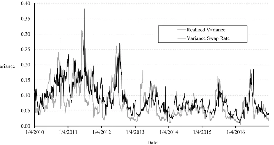
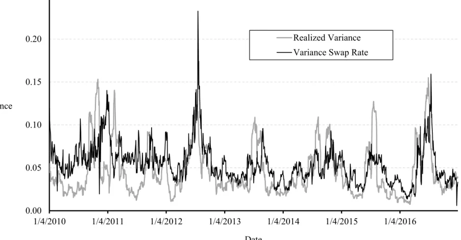
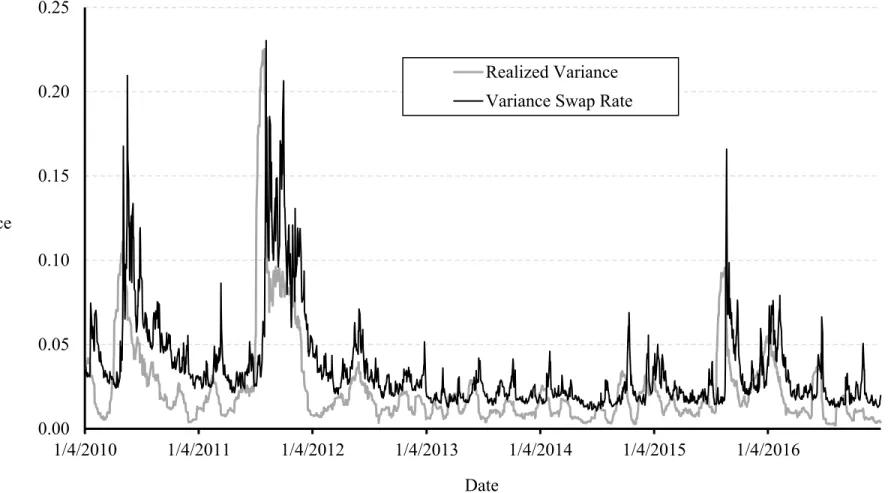
Figures 1 through 3 depict the time series of the variance swap rate and the realized variance for corn, soybean, and the S&P 500 Index, respectively. For all three assets, the realized variance and the variance swap rate are fairly close, with the former usually smaller than the latter, but this tendency is less conspicuous for corn and soybean. All three figures show that, although the two series tend to move together overall, their changes over shorter intervals (e.g., daily changes) are much less similar. In addition, in contrast to the volatility for the S&P 500 Index, volatilities for corn and soybean tend to exhibit some regular seasonal patterns, with the variance having a tendency to be larger over the periods corresponding to the growing season.

More interestingly, the variance swap rate series seem to lag the realized variance series. Intuitively, this is because, as shown in equation (1), the realized variance at date t (RVt,t+30∆) is

calculated using the futures price realizations over in the next 22 business days (F(t, T), …, F(t +

4 _{For more details please refer to https://www.quandl.com/collections/futures/continuous.}

5 _{Options expire every month, whereas futures expire only in certain months. Therefore, in some instances futures}

expire after options do, and the futures whose prices are used to calculate the realized variances are not necessarily the futures underlying the options used to construct the volatility index during a short period right before the delivery dates.

22 ∆, T)), and will remain unknown until the end of that period. In contrast, the date-t variance swap rates are computed from the option prices observed at t. Since people cannot fully predict the futures price behavior, they may naturally rely on the most recent market conditions to price options. As a result, the current variance swap rate (SVt,t+30∆) is likely to contain similar

information as the realized variance 22 business days earlier (RVt−30∆,t), which is likely to cause

the lag.

To better assess the apparent association between the variance swap rate and the lagged realized variance, in Figure 4 we show the correlation between the two series as a function of the number of days in the lag, i.e., the correlation between SVt,t+30∆ and RVt−j∆,t+(30-j)∆ as a function of

j. For all the three assets, correlations increase with the number of days in the lag until they reach a plateau at between 10 and 20 business days in the lag; beyond that interval, correlations decline with the number of days in the lag. This finding supports our conjecture that the variance swap rate is dependent on the more recent market events, and tends to mimic the behavior of the most recently observed realized variance. We also notice that the S&P 500 Index has the largest correlation, followed by corn and soybean. This finding suggests that the variance swap rate is a better track of the realized variance in the equity market than in the agricultural markets.

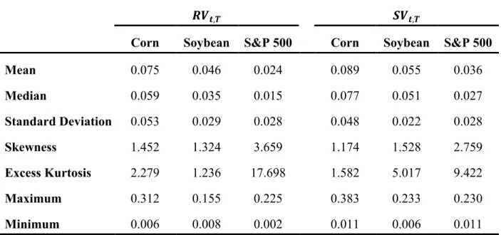
Table 1 provides summary statistics on the realized variance and variance swap rate. Although the results are reported as variances, they can be easily transformed into volatilities by taking the square root. Taking corn as an example, mean RV = 0.075 and mean SV = 0.089 are equivalent to annualized volatilities of 0.0750.5 _{= 27.4% and 0.089}0.5 _{= 29.8%, respectively. The}

mean variance swap rate is larger than the mean realized variance in all the three markets, which implies that the variance risk premium in dollar terms is negative, thus indicating that the

variance risk is priced in the equity market as well as in the agricultural markets. Corn is the most volatile market, as it exhibits the largest mean and median for both realized variance and variance swap rate, followed by soybean; the S&P 500 Index is clearly the least volatile. Furthermore, corn also has the highest volatility of variance, as indicated by the standard

deviation of the realized variance and the variance swap rate. All three assets have positive skewness and excess kurtosis, but corn and soybean are generally less skewed with thinner tails.

Next, we will study the commonalities across the three markets. In particular, we will focus on the daily changes in variances and prices. Figures 1 through 3 hint that the

contemporaneous correlations between the daily changes in the variance swap rates and the realized variances are low, which is consistent with the aforementioned finding that the variance swap rate series lag the realized variance series. In fact, the contemporaneous correlations

between daily changes in the variance swap rates and the realized variances are not even positive for any of the three assets; specifically, the correlations are −0.07 for corn, −0.04 for soybean, and −0.23 for the S&P 500 Index.

Given the negative (albeit negligible for corn and soybean) correlation between the contemporaneous daily changes in the variance swap rates and the realized variances, we

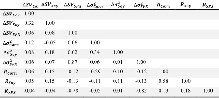
examine the correlations between the contemporaneous daily changes in the variance swap rates and the corresponding conditional variances estimated from an EGARCH(1, 1) model (e.g., Nelson 1991). Similar to the variance swap rates, the EGARCH estimated variances are based on the underlying asset prices, but they are not cumulative over one-month periods and are more likely to align with the variance swap rates. Table 2 presents the correlations between

contemporaneous daily changes in variance swap rates (∆SV), daily changes in the EGARCH(1,

1) estimated variances (∆σ2_{), and the daily log returns of the underlying assets (R) for all the}

three markets.

The figures reported in Table 2 reveal some interesting patterns. First, changes in corn and soybean variance swap rates are moderately correlated (correlation = 0.32), but both are nearly uncorrelated with changes in the variance swap rate of the S&P 500 Index. Changes in EGARCH estimated variances follow a similar pattern, with moderate correlation (0.34) between corn and soybean, but essentially no correlation between either corn or soybean and the S&P 500 Index. Second, unlike the S&P 500 Index, whose changes in variance swap rates and changes in EGARCH estimated variances are highly correlated (correlation = 0.87), corn and soybean

exhibit relatively weak correlations (0.12 and 0.18, respectively) between the changes in these two variance measures. Finally, as expected, the S&P 500 Index displays a highly negative correlation between returns and changes in variance (-0.78 for variance swap rates and

-0.82 for EGARCH estimated variances), which is known as the leverage effect, a phenomenon discussed in many previous studies (e.g., Christie 1982). In contrast, the correlations between returns and changes in variances for corn and soybean are not only of much smaller magnitude (absolute values ranging between 0.06 and 0.29), but also positive except for the correlation between corn returns and changes in corn’s EGARCH estimated variances. Therefore, the corn and soybean markets do not seem to be characterized by a leverage effect.

4.1. Variance Risk Premia

As previously mentioned, the variance risk premium measures whether and how variance risk is priced in the market, which is estimated in dollar terms as the mean payoff to a long position in the variance swap (i.e., RVt,T−SVt,T), or in log return terms as the sample mean of the log-ratio

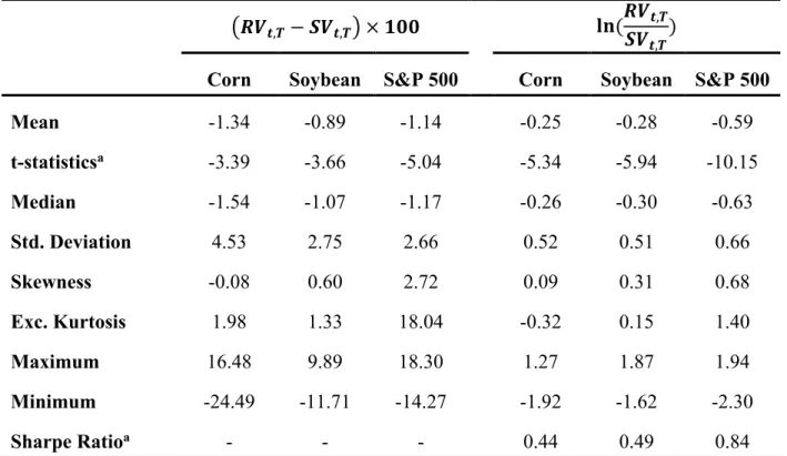
ln(RVt,T/SVt,T). Table 3 reports summary statistics for the variance swap payoffs and log returns

of the S&P 500 Index, corn, and soybean. In particular, the reported payoffs correspond to a long position in the variance swap with a notional value of 100 USD. Also, t-statistics are computed using Newey-West corrected standard deviations with a lag length of 22 business days, to adjust for the serial dependence arising from the overlap in the log returns underlying risk premia separated by 22 or fewer business days. Following the previous literature (e.g., Carr and Wu 2009, Trolle and Schwartz 2010), the lag length chosen as the maturity of the variance swaps is the maximal length of overlap in the series of variance swap rates, i.e., 22 business days for our data. In addition, the autocorrelation functions of the variance swap return also indicate low autocorrelations when the lags are more than 22 business days. In order to understand the

risk-return relationship of the variance swap, we also calculated annualized Sharpe Ratios of shorting the variance swap based on Newey-West corrected standard deviations.6

According to Table 3, the mean payoffs and log returns are negative in all three markets. Newey-West t-statistics indicate statistically significant variance risk premia and log variance risk premia for all the three assets. The S&P 500 Index has the most negative t-statistics for both premia, followed by soybean and corn. Corn has the most negative variance premium in dollar terms, whereas the S&P 500 Index has the most negative log variance risk premium. The discrepancy in ordering comes from the substantial differences in the variance levels across the three assets (see Table 1).

The variance risk premia for corn and soybean shown in Table 3 are consistent with the premia found by Triantafyllou, Dotsis, and Sarris (2015) and Prokopczuk, Symeonidis, and Simen (2017) in that they are negative. However, in Table 3 the magnitude of the corn premia is larger but relatively similar to the soybean premia, both in dollar values and in logarithms, whereas Triantafyllou, Dotsis, and Sarris (2015) (Prokopczuk, Symeonidis, and Simen 2017) found premia substantially larger (smaller) for soybean than for corn.

In practical terms, the fact that the variance risk premia are found to be negative implies that agents view higher market volatility as adversely affecting them. This is true because they are willing to buy variance to reduce their volatility risk (i.e., adopt a long position in the

variance swap), even if that means foregoing average excess returns. Intuitively, the average log variance risk premium of −0.25 for corn can be interpreted as the market overpredicting the volatility of nearby futures by an average of 12.5% (= 0.25/2 × 100). For soybean, the average overprediction is slightly higher at 14.0%, whereas for the S&P Index it is almost double at 29.5%.7 _{That is, the market overestimates the volatility of corn and soybean futures by almost}

6 _{Following Schwarz and Wu (2009), the annualized Sharpe Ratio is computed as SR = (365/30)}0.5

{Avg[−ln(RVt,T/SVt,T)]/NWStdDev[ln(RVt,T/SVt,T]}, where Avg(x) is the average of x, NWStdDev(x) is the

Newey-West corrected standard deviation of x with 22 lags, and the term (365/30)0.5 _{is used to annualize.}

7 _{These estimates of volatility overpredictions are higher than the naïve ones that can be computed from the}

15% on average. This figure is about half the magnitude found for the S&P Index, but it is still quite substantial, and implies that the option premia for corn and soybean have been

“overpriced,” in the sense that they have implied volatilities higher than the historical volatilities. These results have practical implications for U.S. crop insurance programs, because the implied volatilities from the relevant options markets are used to estimate the price volatility factors used to generate premia for revenue insurance products such as RP and RPHPE.Sherrick (2015) has shown that for McLean County Illinois with a corn APH of 180, a 10% increase in the implied volatility causes the producer premium on an RP enterprise policy to increase by 13.3% at the 70% coverage level, 13.4% at the 75% coverage level, 12.7% at the 80% coverage level and 12.1% at the 85% coverage level. The premium increase on a RP policy with harvest price exclusion are even greater at 28.2%, 28.1% 24.2% and 20.7% for the 70 to 85% coverage levels respectively. He reports a similar pattern for soybeans. The results presented above therefore suggest that for the volatility estimate used by RMA is 12.5 to 14% too large. This in turn suggests that producer premia for revenue insurance are overestimated by 15% to 40% for this county and for similar counties. While it was uncertain what caused the overestimate of volatility, our finding suggests that the overestimation existed even when a model-free methodology was employed. Therefore, the high implied volatility was likely to be due to people’s willingness to buy variance to reduce their volatility risk. These variance risk premia should be deducted when calculating implied volatility to avoid overly high insurance prices.

Looking at the distribution of variance swap payoffs, we find fairly low volatility, positive skewness, and excess kurtosis for all three assets. Corn and soybean payoffs are relatively symmetric compared to the S&P 500 Index, and they also have thinner tails. The distributions of log returns are closer to normal, with generally smaller skewness and excess kurtosis, and exhibit slightly negative excess kurtosis for corn and soybean than for the S&P 500 Index.

for soybean, and 20.3% (= −ln(0.024/0.036)/2 × 100) for the S&P 500 Index. The reason for the difference is that the ratio ln(RV /SV ) is itself volatile.

Lastly, the annualized Sharpe Ratio of shorting variance swap is the highest for the S&P 500 Index (0.84), followed by soybean (0.49) and corn (0.44). This result is consistent with the findings of Carr and Wu (2009) and Trolle and Schwartz (2010), who found that the strategy of shorting the S&P 500 Index variance is generally more attractive than shorting variance swaps written on other assets, such as individual stocks and energy commodities. Shorting 30-day corn and soybean variances seems to generate Sharpe Ratios that are comparable to shorting 30-day variances on individual stocks and energy commodities. An interesting finding of Prokopczuk, Symeonidis, and Simen (2017) is that the 90-day Sharpe Ratios are generally lower than 60-day Sharpe Ratios for commodities, suggesting a downward-sloping term structure of the Sharpe Ratio. Specifically, they show the 60-day Sharpe Ratio as 43.7% (22.7%) and the 90-day Sharpe Ratio as 25.7% (5.6%) for corn (soybean) during the period 1989–2011. Although calculated over a different sample period, our 30-day Sharpe Ratios are around 50% for both corn and soybean, implying that the downward-sloping term structure of the Sharpe Ratio may hold for a broader time range.

4.2. Time Variation in Variance Risk Premia

In this section we will test for time variation in the variance risk premia. First, as in Carr and Wu (2009) and Trolle and Schwartz (2010), we will run the following two regressions:

(4) RVt,T = a1 + b1SVt,T + ε1,t,

(5) ln(RVt,T) = a2 + b2ln(SVt,T) + ε2,t.

The null hypothesis for regression in (4) is that the variance risk premium is zero, namely, H0: a1

= 0 and b1 = 1. More precisely, b1 = 1 implies a constant variance risk premium (and therefore

uncorrelated with the variance swap rate), and a1 = 1 further implies that this constant premium

i.e., H0: a2 = 0 and b2 = 1. Both regressions are estimated by OLS using the Newey and West

(1987) estimator with the lag length equal to the variance swap maturity (22 business days) to adjust for autocorrelation.

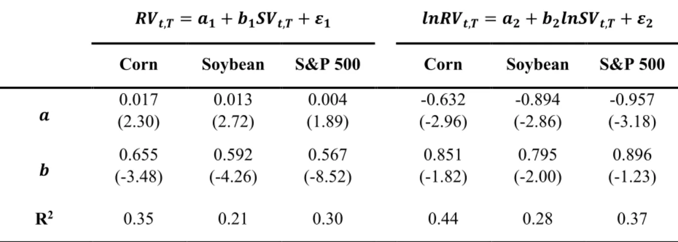
Estimation results are summarized in Table 4. The first three columns report the results of regression (4), and the last three columns report the results of regression (5). The t-statistics under the null hypotheses of aj = 0 and bj = 1 (j = 1, 2) are reported within parentheses. The slope

estimate of regression (4) is significantly smaller than one for all the three assets, which means that (a) corn and soybean variance risk premia in dollar terms are time-varying, and (b) the profitability of shorting the variance swap is positively correlated with the variance swap rate. However, the slope estimates of regression (5) are closer to one, and only significantly different from one at the 95% confidence level for soybean. These findings are consistent with the stock market (Carr and Wu 2009) and energy commodity markets (Trolle and Schwartz 2010).

In the case of corn and the S&P 500 Index, for which the null of constant log variance risk premia cannot be rejected, the intercept estimates reject the null hypothesis of zero log variance risk premia. In conclusion, the difference between the slope estimates of regressions (4) and (5) suggests that the agricultural commodity variance risk premia in terms of log returns are more likely to be constant than in dollar terms, especially for corn. In addition, the R2 _is

considerably higher for (5) than for (4), suggesting that (5) is a better model.

Next, we will test the same relationship taking into account the measurement error existing in the synthetic variance swap rate. Measurement errors may distort the estimation results of regression (4) and make our conclusion unreliable. As in Carr and Wu (2009), we assume the true unobservable variance swap rate to be SVt,T and the synthetic observable swap

rate to be SVt T, , then the measurement error et is the difference between these two, that is, et =

_{t T,}

SV −SVt,T. Alternatively, the regression is expanded to the following:

(6) _ , ,         t T t T RV SV = 0       a + 1       b SVt,T +   

ε

Furthermore, we propose an AR(1) specification for SVt,T, as follows:

(7) SVt,T = φθ + (1 −φ) SVt−1,T + ut.

The error terms (εt, et, ut) are assumed to be normally distributed with variances (

σ

σ

σ

The AR(1) model (7) can be re-written as ∆SVt,T = φ (θ−SVt−1,T ) + ut to make it clear that it is

the discrete time analog of a continuous Ornstein-Uhlenbeck process, with θ representing the long-term mean and φ measuring the rate of mean reversion.8

We use the Kalman filter (Durbin and Koopman 2012) and maximum likelihood

estimation (MLE) to compute the parameters. Specifically, the state model is represented by the measurement equations (6) and the transition equation (7). In order to consider the correlation between the error terms (εt, et), we perform the estimation in two steps. In the first step, we

assume the error terms to be distributed independently and calculate the parameters by means of MLE. In this step, we use the results in Table 4 together with educated guesses to provide initial values of the parameters, as well as the initial state estimate and its variance required by Kalman filter. In the second step, we compute the correlation between the error terms εt and et computed

in the first step, and re-estimate the model imposing such correlation in the variance-covariance matrix. Additionally, in the second step we update the initial values of other parameters based on the estimation results from the first step.

Estimation results are displayed Table 5. The slope estimates for corn, soybean, and the S&P 500 Index are 0.681, 0.592, and 0.575, respectively. These estimates are slightly smaller compared to the ones without taking correlations into account, which are 0.699, 0.610, and 0.603, respectively. Note that the MLE slope estimates without considering correlations are

8 _{The interpretation of φ is that the process SVt,T reverts to the mean θ by approximately (100 φ)% per unit of time.}

For example, as shown later in Table 5, estimation of equation (7) using daily corn data yields φ = 0.0199 and θ = 0.086; hence, SVt,T for corn reverts back to the mean value of 0.086 by about 2% in one day. Note that the mean

higher and closer to one than the OLS slope estimates for all the three assets (see Table 4). This is also the case for selected stock indexes as in Carr and Wu (2009). The difference between the two estimates is due to the measurement errors in the synthetic variance swap rates, which give rise to a slight underestimation of the correlation between variance risk premia and variance swap rates. After considering the correlation between the error terms εt and et, the MLE slope

estimates are still higher than the OLS slope estimates for corn and the S&P 500 Index, and are of the same magnitude for soybean. In summary, the conclusion of time-varying variance risk premia in dollar terms is still valid after correcting for measurement bias.

4.3. Variance Risk Premia vs. Price Risk Premia

In this section we examine whether the variance risk premium is induced by the price (return) risk premium, or whether it represents an independent source of risk. In particular, we regress the log return to a long position in the variance swap on the annualized log return of the underlying asset over the life of the swap. The regressor is defined as

(8) Rt,t+30∆≡ 1 22∆ 22 1 ( , ) [ ( )]. ( ( 1) , ) = + ∆ + − ∆

∑

The null hypothesis is a zero slope estimate, i.e., that the variance risk premium is not linked to the price risk. As before, we use the Newey and West (1987) estimator with the lag length equal to the variance swap maturity (22 business days) to adjust for autocorrelation.

Regression results are presented in the first three columns of Table 6. According to the t-statistics corresponding to the slope estimates, corn shows a negligibly small and non-significant relationship between the log variance risk premium and the return to the underlying asset, and soybean exhibits a small negative and barely significant relationship, whereas the S&P 500 Index shows a large negative and highly significant relationship. The R2 _{is very small for both corn and}

negative for all three assets, and nearly identical to the respective mean log variance risk premia reported in Table 3. This result should not be surprising, because the mean log returns of the underlying assets are very close to zero (and, in addition, for corn and soybean the slopes are very small).

In addition, we fitted two more regressions by dividing the observations into two subsamples, one with only positive returns and the other one with only negative returns. The estimation results are reported in columns 4-6 and 7-9, respectively, of Table 6. Interestingly, both corn and soybean display a significantly negative relationship between variance swap returns and futures returns when futures returns are negative, and a significantly positive

relationship between variance swap returns and futures returns when futures returns are positive. That is, there is a strong non-linear relationship for these two assets, which helps explain the weak linear relationship when regressing across the entire sample. Alternatively, the log swap returns for corn and soybean tend to increase with the absolute magnitude of the underlying log futures returns. In contrast, there are significantly negative relationships in all the three

regressions for the S&P 500 Index.9 _{Furthermore, the R}2 _{and the absolute value of the slope}

coefficients are much larger for the S&P Index regressions than for the corn and soybean regressions.

In summary, variance and price risk premia are weakly correlated overall and exhibit strong non-linearity for corn and soybean, suggesting that the variance risk is unspanned by commodity futures. The slope estimates are significant when dividing the observations into two subsamples based on the return sign, but the relatively low R2 _{of the regressions indicates that}

futures return explain only a small proportion of the variability in the commodity variance swap returns. As is stated in most previous works, variance risk is an independent source of risk needing further investigation.

9 _{Our results for the S&P 500 Index are slightly different from Trolle and Schwartz (2010), in that they found a}

statistically highly significant negative relationship between variance swap returns and the index returns when the index returns are negative, but a non-significant relationship when the index returns are positive.

5. Conclusion

In this paper we make use of the newly released corn and soybean volatility indexes from the CME group to obtain the variance swap rate, a model-free measure of return variance, and investigate variance risk premia in these markets. We find that variance risk is negatively priced for both agricultural commodities, but more statistically significant so for soybean than for corn. We also find commonalities in variance within the agricultural sector and relatively weak

correlation between return and variance for corn and soybean, as opposed to the leverage effect in the equity market. The variance swap rate tends to lag the realized variance series by about 20 business days, and is a better track of the realized variance in the equity market than in the agricultural markets. In addition, corn and soybean variance risk premia in dollar terms are time-varying and correlated with the variance swap rate, which is supported by estimation results with and without measurement errors taken into account. In contrast, agricultural commodity variance risk premia in terms of log return are more likely to be constant and less correlated with the log variance swap rate. Furthermore, variance and price (return) risk premia are weakly correlated, and the correlation depends on the sign of the return. This finding suggests that the variance risk is unspanned by commodity futures and is an independent source of risk needing further

investigation.

The empirical results suggest that the implied volatilities in corn and soybean futures market overestimate true expected volatility by approximately 15%. This has implications for derivative products, such as revenue insurance, that use these implied volatilities to calculate fair premia. More specifically, the USDA Risk Management Agency computes premia for revenue insurance products based on the implied volatilities in the relevant options markets. According to Sherrick (2015), larger than warranted implied volatilities have caused revenue insurance premia for some Illinois counties to be overestimated by as much as 40%. The present findings suggest that the likely culprit for the overestimation is the variance (volatility) risk premium, and that the estimated volatility should be adjusted to avoid the overvaluation of insurance premia.

References

Assa, H. 2016. “Financial Engineering in Pricing Agricultural Derivatives Based on Demand and Volatility.” Agricultural Finance Review 76 (1):42-53.

Barone-Adesi, G., and R.E. Whaley. 1987. “Efficient Analytic Approximation of American Option Values.” Journal of Finance 42(2):301-320.

Buguk, C., D. Hudson, and T.R. Hanson. 2003. “Price Volatility Spill-Over in Agricultural Markets: An Examination of U.S. Catfish Markets” Journal of Agricultural and Resource Economics 28(1):86-99.

Carr, P., and L. Wu. 2009. “Variance Risk Premiums.” Review of Financial Studies 22:1311-1341.

Carr, P., and D. Madan. 1998. “Towards a Theory of Volatility Trading.” In R. Jarrow, ed.,

Volatility: New Estimation Techniques for Pricing Derivatives, pp. 417-427. London: Risk Books.

Cashin, P., and C.J. McDermott. 2002. “The Long-run Behavior of Commodity Prices: Small Trend and Big Variability.” IMF Staff Papers 49(2):175-199.

Chicago Board Options Exchange (CBOE). 2014. “VIX White Paper.” Available at

http://www.cboe.com/micro/VIX/vixwhite.pdf. Accessed June 26, 2017.

Chicago Mercantile Exchange (CME) Group. 2012. “Frequently Asked Questions about CME Group Volatility Indexes.” Available at

http://www.cmegroup.com/trading/options-volatility-indexes.html.Accessed February 17, 2014.

Christie, A.A. 1982. “The Stochastic Behavior of Common Stock Variances: Value, Leverage and Interest Rate Effects.” Journal of Financial Economics 10(4):407-432.

Deaton, A., and G. Laroque. 1992. “On the Behaviour of Commodity Prices.” Review of Economic Studies 59:1-23.

Durbin, J., and S.J. Koopman. 2012. Time Series Analysis by State Space Methods, Second Edition. Oxford, United Kingdom: Oxford University Press.

Geman, H. 2014. Agricultural Finance: From Crops to Land, Water and Infrastructure. John Wiley & Sons, 2014.

Gilbert, C.L. 2006. “Trends and Volatility in Agricultural Commodity Prices.” In Sarris, A., and D. Hallam, eds., Agricultural Commodity Markets and Trade: New Approaches to Analyzing Market Structure and Instability, Ch. 2, pp. 31-60. Northampton, MA: Edward Elgar

Publishing.

Giot, P. 2003. “The Information Content of Implied Volatility in Agricultural Commodity Markets.” Journals of Futures Markets 23(5):441-454.

Nelson, D.B. 1991. “Conditional Heteroskedasticity in Asset Returns: A New Approach.”

Econometrica 59(2):347-370.

Prokopczuk, M., L. Symeonidis, and C.W. Simen. 2017. “Variance Risk in Commodity Markets.” Journal of Banking and Finance 81:136-149.

Sherrick, B. 2015. “Understanding the Implied Volatility (IV) Factor in Crop Insurance.” farmdoc daily (5):37, Department of Agricultural and Consumer Economics, University of Illinois at Urbana-Champaign, February 27. Available at

https://farmdocdaily.illinois.edu/2015/02/understanding-implied-volatility-crop-insurance.html

Stokes, J.R. 2000. “A Derivative Security Approach to Setting Crop Revenue Coverage Insurance Premiums.” Journal of Agricultural and Resource Economics 25(1):159-176. Triantafyllou, A., G. Dotsis, and A.H. Sarris. 2015. “Volatility Forecasting and Time-Varying

Variance Risk Premiums in Grain Commodity Markets.” Journal of Agricultural Economics

66(2):329-357.

Trolle, A., and E.S. Schwartz. 2010. “Variance Risk Premia in Energy Commodities.” Journal of Derivatives 17:15-32.

Turvey, C.G. 1992. “Contingent Claim Pricing Models Implied by Agricultural Stabilization and Insurance Policies.” Canadian Journal of Agricultural Economics 40(2):183-198.

Turvey, C.G., and J.R. Stokes. 2008. “Market Structure and the Value of Agricultural Contingent Claims.” Canadian Journal of Agricultural Economics 56 (1):79-94.

Turvey, C. G., J. Woodard, and E. Liu. 2014. “Financial Engineering for the Farm Problem.”

Agricultural Finance Review 74(2):271-286.

Wang, Z., S. Fausti., and B. Qasmi. 2010. “Variance Risk Premiums and Predictive Power of Alternative Forward Variances in the Corn Market.” Journal of Futures Markets 32(6):587-608.

Appendix: Computation of the Realized Variance for Corn

The following spreadsheet table shows the computation of the realized variance for corn over the period 11/29/2010 through 1/3/2011.Future1 is the nearby corn futures in cents/bu. Future2 is the corn futures maturing immediately after Future1 does; Future2 is reported only for the last 8 days before expiration of Future1. AdjFuture is equal to (Future1 × Weight1 + Future2 ×

Weight2) over the last 8 days before expiration of Future1, and is equal to Future1 otherwise. DailyLR is the daily log return, ARV denotes the annualized realized variance, and ALR the annualized log return (i.e., equation (8) in the text). The Excel formulas for cells G2, H2, and I2 are “=LN(F4/F3)”, “=SUMSQ(G3:G24)*252/22”, and “=SUM(G3:G24)*252/22”, respectively.

A B C D E F G H I

1 Date Future1 Weight1 Future2 Weight2 AdjFuture DailyLR ARV ALR 2 11/29/2010 538.25 0 538.25 -0.01545 0.068104 1.545491 3 11/30/2010 530 0 530 0.040218 0.070368 1.96164 4 12/1/2010 551.75 0 551.75 -0.02014 0.05396 1.345114 5 12/2/2010 540.75 0 540.75 0.03607 0.053683 1.352093 6 12/3/2010 573.5 0.11111 559 0.88889 560.6111 -0.00661 0.042293 1.139517 7 12/6/2010 568 0.22222 553.75 0.77778 556.9167 -0.00872 0.050935 0.891643 8 12/7/2010 561.75 0.33333 547.25 0.66667 552.0833 0.025189 0.051631 0.857515 9 12/8/2010 574.5 0.44444 559.5 0.55556 566.1667 0.003282 0.04893 0.797698 10 12/9/2010 574.25 0.55556 560.25 0.44444 568.0278 0.002735 0.048807 0.760106 11 12/10/2010 574.25 0.66667 560.25 0.33333 569.5833 0.027656 0.065945 1.172954 12 12/13/2010 588.5 0.77778 575.25 0.22222 585.5556 0.000474 0.06092 1.063048 13 12/14/2010 587.25 0.88889 574.5 0.11111 585.8333 -0.00271 0.061991 1.168502 14 12/15/2010 584.25 0 584.25 0.005547 0.065001 1.387753 15 12/16/2010 587.5 0 587.5 0.015203 0.073669 1.002767 16 12/17/2010 596.5 0 596.5 0.005017 0.075462 1.05414 17 12/20/2010 599.5 0 599.5 0.004577 0.075455 1.053457 18 12/21/2010 602.25 0 602.25 0.011146 0.075321 0.966124 19 12/22/2010 609 0 609 0.008177 0.077334 0.640085 20 12/23/2010 614 0 614 0.002034 0.08168 0.788416 21 12/27/2010 615.25 0 615.25 0.012919 0.082944 0.642564 22 12/28/2010 623.25 0 623.25 0.001203 0.082278 0.375148 23 12/29/2010 624 0 624 -0.0129 0.08874 0.633798 24 12/30/2010 616 0 616 0.020884 0.087935 0.893944 25 12/31/2010 629 0 629 -0.01361 0.083211 0.710485 26 1/3/2011 620.5 0 620.5 -0.01953 0.082267 0.750215

Table 1. Summary Statistics of Realized Variance (𝑹𝑹𝑹𝑹𝒕𝒕,𝑻𝑻) and Variance Swap Rate (𝑺𝑺𝑹𝑹𝒕𝒕,𝑻𝑻)

𝑹𝑹𝑹𝑹𝒕𝒕,𝑻𝑻 𝑺𝑺𝑹𝑹𝒕𝒕,𝑻𝑻

Corn Soybean S&P 500 Corn Soybean S&P 500

Mean 0.075 0.046 0.024 0.089 0.055 0.036 Median 0.059 0.035 0.015 0.077 0.051 0.027 Standard Deviation 0.053 0.029 0.028 0.048 0.022 0.028 Skewness 1.452 1.324 3.659 1.174 1.528 2.759 Excess Kurtosis 2.279 1.236 17.698 1.582 5.017 9.422 Maximum 0.312 0.155 0.225 0.383 0.233 0.230 Minimum 0.006 0.008 0.002 0.011 0.006 0.011

Note: The VIX index is stated as percentage points per annum. Hence, the variance swap rate is calculated as

Table 2. Correlations of Daily Variance Changes and Returns for Corn, Soybean and S&P 500 Index ∆𝑺𝑺𝑹𝑹𝑪𝑪𝑪𝑪𝑪𝑪 ∆𝑺𝑺𝑹𝑹𝑺𝑺𝑪𝑪𝑺𝑺 ∆𝑺𝑺𝑹𝑹𝑺𝑺𝑺𝑺𝑺𝑺 ∆𝝈𝝈𝑪𝑪𝑪𝑪𝑪𝑪𝑪𝑪𝟐𝟐 ∆𝝈𝝈𝑺𝑺𝑪𝑪𝑺𝑺𝟐𝟐 ∆𝝈𝝈𝑺𝑺𝑺𝑺𝑺𝑺𝟐𝟐 𝑹𝑹𝑪𝑪𝑪𝑪𝑪𝑪𝑪𝑪 𝑹𝑹𝑺𝑺𝑪𝑪𝑺𝑺 𝑹𝑹𝑺𝑺𝑺𝑺𝑺𝑺 ∆𝑺𝑺𝑹𝑹𝑪𝑪𝑪𝑪𝑪𝑪𝑪𝑪 1.00 ∆𝑺𝑺𝑹𝑹𝑺𝑺𝑪𝑪𝑺𝑺 0.32 1.00 ∆𝑺𝑺𝑹𝑹𝑺𝑺𝑺𝑺𝑺𝑺 0.06 0.08 1.00 ∆𝝈𝝈𝑪𝑪𝑪𝑪𝑪𝑪𝑪𝑪𝟐𝟐 0.12 -0.05 0.06 1.00 ∆𝝈𝝈𝑺𝑺𝑪𝑪𝑺𝑺𝟐𝟐 0.08 0.18 0.02 0.34 1.00 ∆𝝈𝝈_{𝑺𝑺𝑺𝑺𝑺𝑺}𝟐𝟐 _{0.06 0.07 0.87 0.06 0.01 1.00} 𝑹𝑹𝑪𝑪𝑪𝑪𝑪𝑪𝑪𝑪 0.06 0.15 -0.12 -0.29 0.10 -0.12 1.00 𝑹𝑹𝑺𝑺𝑪𝑪𝑺𝑺 0.05 0.15 -0.13 -0.11 0.11 -0.13 0.58 1.00 𝑹𝑹𝑺𝑺𝑺𝑺𝑺𝑺 -0.04 -0.04 -0.78 -0.05 0.01 -0.82 0.13 0.18 1.00

Table 3. Summary Statistics for the Variance Risk Premium

�𝑹𝑹𝑹𝑹𝒕𝒕,𝑻𝑻− 𝑺𝑺𝑹𝑹𝒕𝒕,𝑻𝑻�×𝟏𝟏𝟏𝟏𝟏𝟏 𝐥𝐥𝐥𝐥 (𝑹𝑹𝑹𝑹_{𝑺𝑺𝑹𝑹}𝒕𝒕,𝑻𝑻

𝒕𝒕,𝑻𝑻)

Corn Soybean S&P 500 Corn Soybean S&P 500

Mean -1.34 -0.89 -1.14 -0.25 -0.28 -0.59 t-statisticsa _{-3.39 -3.66 -5.04 -5.34 -5.94 -10.15} Median -1.54 -1.07 -1.17 -0.26 -0.30 -0.63 Std. Deviation 4.53 2.75 2.66 0.52 0.51 0.66 Skewness -0.08 0.60 2.72 0.09 0.31 0.68 Exc. Kurtosis 1.98 1.33 18.04 -0.32 0.15 1.40 Maximum 16.48 9.89 18.30 1.27 1.87 1.94 Minimum -24.49 -11.71 -14.27 -1.92 -1.62 -2.30 Sharpe Ratioa _{- - - 0.44 0.49 0.84}

a_{The t-statistics and the Sharpe Ratio are computed using Newey-West corrected standard deviations with a lag} length of 22 business days.

Table 4. Time Variation in Variance Risk Premia

𝑹𝑹𝑹𝑹𝒕𝒕,𝑻𝑻 =𝒂𝒂𝟏𝟏+𝒃𝒃𝟏𝟏𝑺𝑺𝑹𝑹𝒕𝒕,𝑻𝑻+𝜺𝜺𝟏𝟏 𝒍𝒍𝑪𝑪𝑹𝑹𝑹𝑹𝒕𝒕,𝑻𝑻 =𝒂𝒂𝟐𝟐+𝒃𝒃𝟐𝟐𝒍𝒍𝑪𝑪𝑺𝑺𝑹𝑹𝒕𝒕,𝑻𝑻+𝜺𝜺𝟐𝟐

Corn Soybean S&P 500 Corn Soybean S&P 500

𝒂𝒂 _(2.30) 0.017 _(2.72) 0.013 _(1.89) 0.004 _(-2.96) -0.632 _(-2.86) -0.894 _(-3.18) -0.957 𝒃𝒃 _(-3.48) 0.655 _(-4.26) 0.592 _(-8.52) 0.567 _(-1.82) 0.851 _(-2.00) 0.795 _(-1.23) 0.896

R2 _{0.35 0.21 0.30 0.44 0.28 0.37}

Note: t-Statistics under the null hypotheses of 𝑎𝑎𝑖𝑖= 0 and 𝑏𝑏𝑖𝑖= 1 (𝑖𝑖= 1,2) are reported in parentheses. t-statistics are

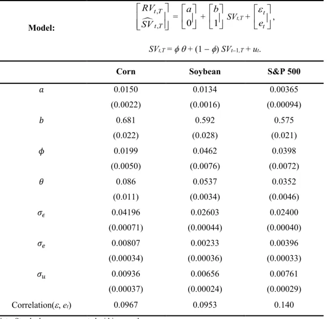
Table 5. Kalman Filter Maximum Likelihood Estimates of Time Variationin Variance Risk Premia Model:  , ,         t T t T RV SV = 0       a + 1       b SVt,T +   

ε

Corn Soybean S&P 500

𝑎𝑎 0.0150 (0.0022) 0.0134 (0.0016) 0.00365 (0.00094) 𝑏𝑏 0.681 (0.022) 0.592 (0.028) 0.575 (0.021) 𝜙𝜙 0.0199 (0.0050) 0.0462 (0.0076) 0.0398 (0.0072) 𝜃𝜃 0.086 (0.011) 0.0537 (0.0034) 0.0352 (0.0046) 𝜎𝜎𝜖𝜖 0.04196 (0.00071) 0.02603 (0.00044) 0.02400 (0.00040) 𝜎𝜎𝑒𝑒 0.00807 (0.00034) 0.00233 (0.00036) 0.00396 (0.00033) 𝜎𝜎𝑢𝑢 0.00936 (0.00037) 0.00656 (0.00024) 0.00761 (0.00029) Correlation(ε, et) 0.0967 0.0953 0.140

Table 6. Variance Risk Premia vs. Price Risk Premia

𝐥𝐥𝐥𝐥 (𝑹𝑹𝑹𝑹𝒕𝒕,𝑻𝑻

𝑺𝑺𝑹𝑹𝒕𝒕,𝑻𝑻) =𝜶𝜶+𝜷𝜷𝑅𝑅𝑡𝑡,𝑇𝑇+𝜺𝜺

(𝑅𝑅𝑡𝑡,𝑇𝑇 < 0)∪(𝑅𝑅𝑡𝑡,𝑇𝑇 ≥0) 𝑅𝑅𝑡𝑡,𝑇𝑇 < 0 𝑅𝑅𝑡𝑡,𝑇𝑇 > 0

Corn Soybean S&P 500 Corn Soybean S&P 500 Corn Soybean S&P 500

𝜶𝜶 _(-5.34) -0.252 _(-5.99) -0.280 _(-11.68) -0.491 _(-6.94) -0.421 _(-8.04) -0.536 _(-9.04) -0.507 _(-4.86) -0.371 _(-8.12) -0.539 _(-9.41) -0.646 𝜷𝜷 _(-0.29) -0.012 _(-1.27) -0.089 _(-9.90) -0.990 _(-4.71) -0.219 _(-7.19) -0.484 _(-7.70) -1.135 _(2.56) 0.171 _(3.298) 0.402 _(-3.66) -0.587

R2 _{0.001 0.02 0.44 0.09 0.28 0.39 0.04 0.11 0.08}

Note: t-Statistics under the null hypotheses of 𝜶𝜶= 0 and 𝜷𝜷= 0 are reported in parentheses. t-statistics are computed using Newey-West corrected standard deviations with a lag length of 22 business days.

Figure 1: Variance swap rate and realized variance for corn. 0.00 0.05 0.10 0.15 0.20 0.25 0.30 0.35 0.40 1/4/2010 1/4/2011 1/4/2012 1/4/2013 1/4/2014 1/4/2015 1/4/2016 Variance Date Realized Variance Variance Swap Rate

Figure 2: Variance swap rate and realized variance for soybeans. 0.00 0.05 0.10 0.15 0.20 0.25 1/4/2010 1/4/2011 1/4/2012 1/4/2013 1/4/2014 1/4/2015 1/4/2016 Variance Date Realized Variance Variance Swap Rate

Figure 3: Variance swap rate and realized variance for S&P500. 0.00 0.05 0.10 0.15 0.20 0.25 1/4/2010 1/4/2011 1/4/2012 1/4/2013 1/4/2014 1/4/2015 1/4/2016 Variance Date Realized Variance Variance Swap Rate

Figure 4: Correlation between variance swap rate and lagged realized variance, as a function of the number of days in the lag. 0.00 0.10 0.20 0.30 0.40 0.50 0.60 0.70 0.80 0.90 0 2 4 6 8 10 12 14 16 18 20 22 24 26 28 30 32 34 36 38 40 42 44 46 48 50 52 54 56 58 60 Correlation

Number of Days in the Lag Correlation for Corn

Correlation for Soybean Correlation for SPX