2018
Information transfer in dynamical systems
Subhrajit Sinha
Iowa State University
Follow this and additional works at:
https://lib.dr.iastate.edu/etd
Part of the
Electrical and Electronics Commons
This Dissertation is brought to you for free and open access by the Iowa State University Capstones, Theses and Dissertations at Iowa State University Digital Repository. It has been accepted for inclusion in Graduate Theses and Dissertations by an authorized administrator of Iowa State University Digital Repository. For more information, please [email protected].
Recommended Citation
Sinha, Subhrajit, "Information transfer in dynamical systems" (2018).Graduate Theses and Dissertations. 16468.
by
Subhrajit Sinha
A dissertation submitted to the graduate faculty in partial fulfillment of the requirements for the degree of
DOCTOR OF PHILOSOPHY
Major: Electrical Engineering
Program of Study Committee: Umesh Vaidya, Major Professor
Nicola Elia Venkataramana Ajjarapu Baskar Ganapathysubramanian
Soumik Sarkar
The student author, whose presentation of the scholarship herein was approved by the program of study committee, is solely responsible for the content of this dissertation. The Graduate College will
ensure this dissertation is globally accessible and will not permit alterations after a degree is conferred.
Iowa State University Ames, Iowa
2018
DEDICATION
I would like to dedicate my thesis to all the wonderful teachers I have had over the years, without whom I would not have learned to ask questions.
TABLE OF CONTENTS
LIST OF TABLES . . . vii
LIST OF FIGURES . . . viii
ACKNOWLEDGEMENTS . . . xiii
ABSTRACT . . . xiv
CHAPTER 1. INTRODUCTION . . . 1
1.1 Previous Work . . . 1
1.2 Our Contribution . . . 4
1.3 Organization of the Report . . . 6
CHAPTER 2. PRELIMINARIES FOR INFORMATION TRANSFER FORMULATION . . . 8
2.1 Perron-Frobenius Operator . . . 9
2.2 Directed Information, Transfer Entropy and Liang-Kleeman Information Transfer . . 10
2.2.1 Directed Information . . . 10
2.2.2 Transfer Entropy . . . 11
2.2.3 Liang-Kleeman Information Transfer . . . 12
CHAPTER 3. INFORMATION TRANSFER . . . 14
3.1 One Step Information Transfer . . . 14
3.1.1 Information Transfer and Causal Inference in Nonlinear Systems . . . 19
3.2 n-step Information Transfer . . . 24
3.3 Information Transfer and Dynamics of Linear Systems . . . 26
CHAPTER 4. INFORMATION TRANSFER IN LINEAR CONTROL SYSTEM . . . 37
4.1 Information Transfer Between the States . . . 37
4.1.1 Examples . . . 41
4.2 Information Transfer in Linear Control Systems . . . 43
4.2.1 Information from Input to State . . . 44
4.2.2 Information from State to Output . . . 44
4.2.3 Information from Input to Output . . . 45
4.3 Information Transfer and Structural Controllability and Observability . . . 46
4.4 Information Transfer in Feedback Control Systems . . . 48
CHAPTER 5. INFORMATION TRANSFER AS A MEASURE OF CAUSALITY . . . 52
5.1 Directed Information as a Measure of Causality . . . 52
5.1.1 Examples . . . 53
5.2 Information Transfer Captures the True Causal Structure . . . 56
CHAPTER 6. EXAMPLES AND APPLICATIONS . . . 58
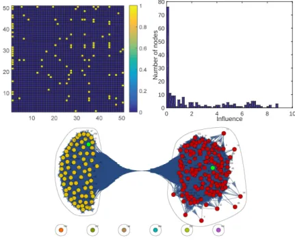
6.1 Application to social network . . . 58
6.1.1 Simulation . . . 59
6.2 Information Transfer and Optimal Placement of Actuators . . . 60
CHAPTER 7. INFLUENCE CHARACTERIZATION IN POWER SYSTEMS . . . 66
7.1 Introduction . . . 66
7.2 Stability Issues in Power Systems . . . 67
7.3 Modelling of a Power Network . . . 68
7.3.1 Generator Model . . . 68
7.3.2 Load Model . . . 70
7.4 Influence Characterization in IEEE 9 Bus System . . . 71
7.4.1 Contribution to most unstable mode . . . 74
7.4.2 Information transfer to the complex modes . . . 78
7.4.3 Information flow from generators to load . . . 79
7.5.1 3 Bus system . . . 82
7.5.2 Information Transfer and Participation Factor . . . 84
7.5.3 Stability and state to state information transfer . . . 85
7.6 IEEE 39 Bus System . . . 86
CHAPTER 8. INFORMATION TRANSFER AND PHASE TRANSITION IN DYNAMICAL SYSTEMS . . . 90
8.1 Information Transfer and Phase Transition . . . 91
8.2 Coupled Oscillators in Double Well Potential . . . 94
8.3 Duffing Oscillator . . . 100
8.4 Lorenz Attractor . . . 102
8.5 Complex Networks . . . 104
CHAPTER 9. CAUSAL INFERENCE FROM TIME SERIES DATA . . . 109
9.1 Transfer operators for stochastic system . . . 109
9.2 Robust approximation of P-F and Koopman operators . . . 111
9.2.1 Robust Optimization, Regularization, and Sparsity . . . 116
9.2.2 Design of robust predictor . . . 117
9.2.3 Examples . . . 119
9.3 Causal Inference in Linear Dynamical System . . . 127
9.3.1 Topology Identification of Linear Networks . . . 131
9.4 Computation of the Information Transfer for Nonlinear Systems . . . 137
9.4.1 Examples and Simulations . . . 140
CHAPTER 10. DATA DRIVEN CAUSAL INFERENCE IN STOCK MARKET . . . 143
10.1 Introduction . . . 143
10.2 Influence in Stock Market . . . 144
10.2.1 Influence between 2 companies . . . 144
10.2.2 Clustering of companies . . . 147
CHAPTER 11. CONCLUSION AND FUTURE WORK . . . 151
11.1 Conclusions . . . 151
11.2 Future Work . . . 151
LIST OF TABLES
Table 7.1 Participation to most unstable mode . . . 75
Table 7.2 Participation to most complex mode . . . 79
Table 7.3 Participation and Information Transfer to most unstable mode . . . 84
LIST OF FIGURES
Figure 3.1 (a) The states are highly correlated. (b) The information transfer between
the states. . . 19
Figure 3.2 A system where two step transfer is non-zero . . . 24
Figure 3.3 (a) Trajectories of the system. (b) IT fromxtoy. . . 27
Figure 3.4 (a) Trajectories of the system. (b) IT fromxtoy. . . 28
Figure 3.5 (a) Trajectories of the system. (b) IT fromxtoy. . . 29
Figure 3.6 (a) Trajectories of the system. (b) IT fromxtoy. . . 29
Figure 3.7 (a) IT fromxtoy. (b) IT fromytox. . . 32
Figure 3.8 (a) Phase space trajectories (b) Invariant measure. (c) Information transfer fromxtoy. (d) Information transfer fromytox. . . 33
Figure 3.9 (a) Information transfer fromxtoy. (b) Information transfer fromytox. . 34
Figure 3.10 (a) Limit cycle forµ= 0.5. (b) Corresponding invariant density. (c) Infor-mation transfer fromxtoy. (d). Information transfer fromytox. . . 35
Figure 4.1 a) RLC series circuit; b) Information transfer between the states . . . 42
Figure 4.2 Mass spring system . . . 43
Figure 4.3 Feedback control system . . . 49
Figure 4.4 (a) N-step information transfer; (b) Average information transfer and average directed information . . . 50
Figure 5.1 (a) Graph of dynamical system of example 1. (b) Graph of dynamical system of example 2. . . 54
Figure 5.2 (a) Directed information plots for example 1. (b) Directed information plots for example 2. . . 54
Figure 5.3 (a) N-step information transfer for example 1. (b) N-step information trans-fer for example 2. . . 56
Figure 6.1 a) Twitter adjacency matrix. b) Distribution of influential nodes. c) Cluster-ing based on influence in Twitter follower network. . . 59
Figure 6.2 (a) Fluid flow vector field. (b)-(d) Eigenvectors corresponding to unit eigen-value of the P-F matrix. . . 64
Figure 6.3 (a) Information transfer between the cells. (b) Optimal location of 200 actu-ators. . . 65
Figure 7.1 IEEE 9 bus network . . . 72
Figure 7.2 P-V curve with operating points . . . 73
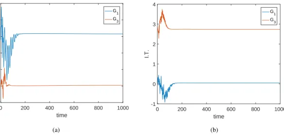
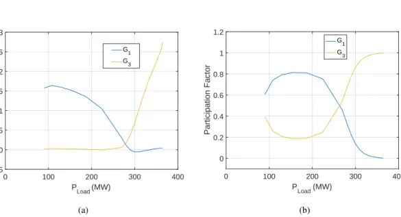
Figure 7.3 Information transfer from generators 1 and 3 to most unstable mode for (a)
Pload= 90MW. (b)Pload = 364.1MW. . . 74
Figure 7.4 (a) Steady state information transfer to most unstable mode from G1 and G3 along operating points. (b) Participation factors of G1 andG3 to most
unstable mode along operating points. . . 76
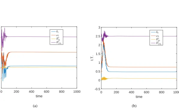
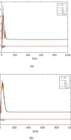
Figure 7.5 (a) Information transfer from individual states ofG1 to most unstable mode
forPload = 90MW. (b) Information transfer from individual states ofG3 to
most unstable mode whenPload = 364.1MW. . . 77
Figure 7.6 Steady state information transfer fromEf d ofG1 andG3 to most unstable
mode along operating points. . . 77
Figure 7.7 Information transfer from states of G3 to complex mode (a) for operating
point 1. (b) for operating point 19. . . 78
Figure 7.8 Information transfer from the generators to the load (a) at operating point 1. (b) at operating point 19. . . 80
Figure 7.9 Steady state values of information transfer fromG1 to load along the
oper-ating points (red curve) and PV curve (black curve). HereV5is the voltage
at bus 5. . . 81
Figure 7.10 Information transfer increases rapidly as the system approaches instability. . 82
Figure 7.11 (a) 3-bus system. (b) Critical points of the system . . . 83
Figure 7.12 (a) IT fromδg beforeS1. (b) IT fromV beforeS3. . . 85
Figure 7.13 IEEE 39 bus system. . . 86
Figure 7.14 (a) Information transfer from generator 10 to generators 1 and 2. (b)Information transfer from generators 5, 8 and 9 to generators 3, 4 and 6 respectively. . . 88
Figure 7.15 (a) Information transfer from generator 10 to generators 1 and 2. (b)Information transfer from generators 1 and 2 to generator 10. . . 89
Figure 8.1 Particle in a symmetric double-well potential. . . 92
Figure 8.2 Phase transformation from ice to water. . . 92
Figure 8.3 (a) Double well potential. (b) Phase portrait of a single oscillator. . . 95
Figure 8.4 Oscillator 1 (marked by red), with massm1 = 100remains in its well and oscillator 2 (marked by yellow) jumps from one well to the other, thus lead-ing to phase transition. . . 96
Figure 8.5 θ2and information transfer when there is only one phase transition. . . 97
Figure 8.6 θ2and information transfer when there are multiple phase transitions. . . . 98
Figure 8.7 θ2and information transfer when there is only one phase transition and there is almost another transition. . . 99
Figure 8.8 Phase portrait of Duffing oscillator . . . 101
Figure 8.9 Information transfer and phase transition in Duffing oscillator. . . 101
Figure 8.10 Phase portrait of Lorenz system. . . 103
Figure 8.11 Information transfer and multiple phase transitions in Lorenz attractor. . . . 104
Figure 8.12 Phase transitions in a 6 node network. . . 105
Figure 8.13 Information transfer in the 6 node network. . . 106
Figure 8.15 (a) Phase transitions in the exponential network. (b) Information transfer in
the 20 node network. . . 108
Figure 9.1 (a) Uncertainty set as intersection of two ellipsoids. (b) Representation of the uncertainty set∆ = [−0.5,0.5]×[−0.5,0.5]. . . 113
Figure 9.2 (a) Dominant eigenvalue comparison when there is no measurement noise. (b) Dominant eigenvalue comparison with both process and measurement noise. . . 120
9.3 (a) Clean data. (b) Noisy data. (c) Comparison of eigenvalues obtained with different algorithms. . . 121
9.4 Sample output trajectory . . . 123
9.5 (a) Eigenvalue comparison of Robust DMD, normal DMD and subspace DMD. (b) Dominant eigenvalues. . . 123
9.6 (a) Eigenvalue comparison of Robust DMD, normal DMD and subspace DMD. (b) Dominant eigenvalues. . . 123
9.7 (a) Error in prediction inrfor initial state at(1,−π). (b) Error in prediction inθinitial state at(1,−π). . . 124
9.8 (a) Average error in prediction ofr. (b) Average error in prediction ofθ. . . 125
9.9 (a) Data generated by Stochastic Burger’s equation with observation noise (b) Eigenvalues of the continuous time system.(c) Zoomed in region of dom-inant eigenvalues captured by the three methods. . . 126
9.10 (a) Error in prediction ofz2. (b) Error in prediction ofz50. (c) Average error in prediction. . . 127
Figure 9.11 Mass-spring-damper system . . . 130
Figure 9.12 Network corresponding to the dynamical system given in (9.34). . . 132
Figure 9.13 Information transfer between the states. . . 132
Figure 9.14 Network identified by Granger causality . . . 133
Figure 9.15 Network obtained using Sparse DMD . . . 134
Figure 9.17 Percentage error in number of links v/s number of nodes. . . 136
Figure 9.18 (a) Support of the eigenfunction corresponding to the largest eigenvalue of the Koopman operator. (b) Support of the eigenfunction corresponding to the second largest eigenvalue of the Koopman operator. . . 141
Figure 10.1 Stock prices of IBM and Intel (INTC). . . 145
Figure 10.2 Stock prices of Coca-cola (KO) and Pepsi (PEP). . . 146
Figure 10.3 Stock prices of At & T (T) and Verizon (VEZ). . . 146
Figure 10.4 Spectral clustering of different banks and computer companies. . . 148
Figure 10.5 Hierarchical clustering of different financial and computer companies. . . . 148
Figure 10.6 Information transfer from (a) American Express (AXP) and (b) Capital One Financial (COF). . . 149
ACKNOWLEDGEMENTS
I would like to take this opportunity to thanks all those who helped me during my research and writing of the thesis. I would particularly like to thank my advisor, Prof. Umesh Vaidya, who allowed me to explore a topic which I had no experience in. The innumerable discussions we had helped me a lot and allowed me to delve in to the beautiful world of entropy, dynamical systems and control theory. I would also like to thank Prof. Ravindra Kulkarni of Indian Institute of Technology, Bombay. It is mostly because of him that I started enjoying geometry and its connections with other branches of mathematics like representation theory, algebra and topology and helped me to learn how to ask questions and be inquisitive. I would also like to thank my teachers in high school, Mr. Partha Pratim Roy and Mr. Mallar Roy for introducing me to the exciting world of classical physics and also Dr. Karthik Basak for teaching me the necessity of understanding the importance of theory in mathematics. I would also like to thank my colleagues, particularly Sai Pushpak and Huang Bowen for accepting me as a colleague and for being there whenever I wanted to discuss my research. Finally, I would like to thank my family and friends for their support throughout my Ph.D. life.
ABSTRACT
Causality analysis has been a topic of research from the days of Aristotle. However, there has not been an universal definition of causality, with different researchers providing different definitions and measures of causality. In this work, we provide a new definition of causality in a dynamical system setting. In particular, we quantify how a state (or subspace) of a dynamical system influence any other state (or subspace). The quantification is in terms of what we call information transfer. Intuitively, information transfer quantifies how the entropy of a state (say y) changes due to evolution of any other state (say x) and this characterizes the causal structure and influence in a dynamical system. We show that the information transfer measure satisfies intuitions of causality and influence. In par-ticular, we show our information transfer measure satisfy (a) zero influence, (b) transfer asymmetry
and(c) information conservation. The one step information transfer is generalized to definen-step information transfer and this enables us to clearly distinguish between direct and indirect influence. With this, we show how in a dynamical system setting, when previous measures of causality fail to capture the true causal structure, our information transfer measure do capture the true causal structure in a dynamical system. Apart from identification of causal structure, we use the information transfer measure to characterize influence and demonstrate how this can be used to characterize stability in a power network. In particular, we show how to identify the states and generators which are responsible for instability of a power network. Moreover, we show how the connection between stability and information transfer can be used to predict phase transitions in complex systems. We also provide two algorithms to compute information transfer from time series data and show how this can be used for topology identification of linear networks and stability analysis of power networks. Finally, as a separate application, we characterize influence in a stock market and also show how the information transfer measure can be used to predict stock market crashes.
CHAPTER 1. INTRODUCTION
Causality and influence characterization is a problem of utmost importance and finds its relevance in many different applications like world wide web and social media, biological networks, neural sci-ence, economics, finance etc. Usually, concepts of information theory are used in such applications and a study of the information flow between the components of the network throws light on causality and the influential nodes of the network. In (1) the authors use information based metric to character-ize the most influential nodes in social networks. In neuroscience, concepts of information theory are used to understand how information flow in different parts of the brain (2) and identifying influence in gene regulatory networks (3; 4) .
Again, Clive Granger, in 1969 (5), provided his own definition of causality to study causality in economic models. This definition of causality, which is now known as Granger causality, is used in economic and financial networks to infer causal interactions from the time series data (6; 7; 8).
Causality detection in system theoretic setting was addressed much later in 2000, when Thomas Schreiber (9) defined transfer entropy between two states in a dynamical system. In 2005, Liang and Kleeman defined information transfer between dynamical system components (10) and provided explicit expressions for the information transfer between the states in a continuous time dynamical system.
1.1 Previous Work
Causality is the agency or efficacy that connects one process (the cause) with another (the effect), where the first is understood to be partly responsible for the second, and the second is dependent on the first. In general, a process has many causes, which are said to be causal factors for it, and all lie in its past. An effect can, in turn, be a cause of many other effects, which all lie in its future. Interpreting
causation as a deterministic relation means that ifA causesB, thenA must always be followed by
B. In this sense, war does not cause deaths, nor does smoking cause cancer or emphysema. As a result, a probabilistic notion of causation is often used. Informally,A(“The person is a smoker”) probabilistically causesB(“The person has now or will have cancer at some time in the future”), if the information thatAoccurred increases the likelihood ofB’s occurrence. This has led the philosophers and researchers to define causality in a probabilistic setting.
However, there has been no universally accepted definition of causality. One of the most com-monly used notions of causality is Granger causality and was proposed by Clive Granger for studying causality in the economics framework and is normally tested in context of linear regression models. For example, consider a bivariate linear autoregressive model of two variablesx1andx2
x1(t) = p X j=1 A11,jx1(t−j) + p X j=1 A12,jx2(t−j) +E1(t) x2(t) = p X j=1 A21,jx1(t−j) + p X j=1 A22,jx2(t−j) +E1(t)
wherep is the maximum number of lagged observations included in the model (the model order), the matrixAcontains the coefficients of the model andE1(t)andE2(t)are the prediction errors for
each time series. If the variance ofE1(orE2) is reduced by the inclusion ofx2(or x1) in the first
(or second) equation, then it is said thatx2(orx1) Granger causesx1(or x2). The usefulness of the
Granger causality lies in the fact that it is easy to use and hence since its development has been used in many different applications (7).
On the other hand, Shannon had defined the entropy of a random variable and developed the field of information theory. However, the information theory, as developed by Shannon, was symmetric and hence one cannot use it directly to infer causality. The concept of mutual information between two random variablexandygives theinformation shared byxandy, but it does not give the direction of flow of information. In order to incorporate the directional sense in information theory, Marko developed what is now known as bi-directional information. It is a natural extension of the concept of mutual information between two random variables and furthermore, it also incorporates the sense of direction. Thus came the idea that elements of information theory can be used to infer the direction of information flow and hence causality. The major breakthrough, however, was achieved by Massey
(11) and later by Kramer (12) who generalized the concept of bi-directional information and defined what is known as directed information.
LetXn ={X1, X2,· · · , Xn}andYn = {Y1, Y2,· · ·, Yn}be two stochastic processes, viewed
as a sequence of random variables. Then the entropy(H)of the random variableXis defined as
H(Xn) =−
Z
ΩX
ρ(Xn) logρ(Xn)dXn (1.1)
whereΩX is the event space of X and ρ(Xn) is the probability distribution of Xn. Massey and
Kramer (12) defined the directed information fromXntoYnas
I(Xn→Yn) =H(Yn)−H(YnkXn) (1.2)
whereH(Yn)is the entropy of the sequenceYnand
H(YnkXn) :=
n X
i=1
H(Yi|Yi−1, Xi) (1.3)
is the entropy ofYncausallyconditioned onXn. The idea ofcausal conditioningtakes into account the direction of information flow and hence throws light on the causal structure of the stochastic process.
The concept of directed information is more suited to stochastic processes and in 2000, Thomas Schreiber proposed the idea of transfer entropy (9) which is geared to study the information flow in systems evolving in time. Transfer entropy is a difference of two conditional entropies and for Markov chains of order one, it is equal to conditional mutual information. The concept of transfer entropy is discussed in chapter2.
However, though transfer entropy was geared more from system theoretic point of view, it fails to capture the zero influence in some cases (13). Liang and Kleeman (10) came up with a new formulation of information transfer in dynamical systems and showed that it captures the notion of zero transfer. To define the Liang-Kleeman information flow from statexto statey, they considered two different systems, namely, the original system and a modified system, where they frozex and propagated the modified system by one-time step to determine the amount of information flow from
xtoy. The Liang-Kleeman information flow is also explained in detail in chapter2.
In (10), the authors had defined Liang-Kleeman information transfer in a two state system. In (14), their definition of information transfer was generalised to define information transfer between
subspaces of dynamical systems with additive noise. Liang and Kleeman carried their research for-ward and studied the information transfer in generaln-dimensional continuous time and discrete time dynamical systems (15; 16; 17). They also studied the information transfer in two dimensional dis-crete time stochastic systems with additive noise (18). In (10), they also show that their formalism of information transfer is qualitatively consistent with the notions of transfer entropy and Granger causal-ity. So Liang-Kleeman information transfer is also used to study the causal structure in a dynamical system. But the Liang-Kleeman information transfer cannot account for indirect transfer (17). Again, transfer entropy, though gives a measure of identifying the direction of information flow, and hence influence, it also suffers from some drawbacks. For example, it may not identify indirect influence and also may give erroneous results in presence of dominant neighbours (13). Directed information, as formulated by Massey and Kramer also suffers from similar deficiencies.
On the other hand, various researchers have tried to connect information theory and control theory. In (19), the authors have studied the classical concepts of controllability and observability from the information theoretic view point. Again, in (20), the authors have shown that the mutual information between the state and the estimate is a maximum in a discrete time Kalman filter. Moreover, in (21), the authors have studied the information flow in a Kalman-Bucy filter.
The main motivation for our work was to come up with a measure of causality which can identify the indirect links and also should be able to correctly infer about the zero influence. Moreover, it would also be nice if the measure of information transfer, so defined to capture the influence structure between the states in a dynamical system, can be extended to define information transfer between the various signals involved in a control system. In that case, it may be possible to connect the information transfer measure with some classic control theoretic notions. In that case, one may be able to connect the two fields of information theory and control theory and study them on a common base.
1.2 Our Contribution
Formalism for information transfer developed in this work is in dynamical systems setting and is closely related to and inspired from information transfer framework developed in (14; 10; 17) for nonlinear dynamical systems. We used the ideas of Liang-Kleeman transfer to propose an axiomatic
definition of information transfer in discrete linear dynamic network (22). The axioms were physically motivated and it was shown in (22) that there exists a unique expression for information transfer in a dynamic network satisfying these axioms. In this work, we use the ideas of directed information and transfer entropy and the intuitions of (10; 22) to define the information transfer.
In particular, instead of absolute entropy, we use the conditional entropy to define the information transfer. This definition is a natural extension of directed information and transfer entropy and we show that the new definition of information transfer satisfies the intuitions of information transfer, namely a) Zero transfer, b) Transfer asymmetry and c) Information conservation. The advantage of using conditional entropy to define information transfer lies in the fact that this new definition of one step information transfer can be naturally extended to definen-step transfer and average information transfer, which can be related to entropy rate of a variable and we find that the extension of the one step information transfer definition to n-step information transfer definition is the precise concept needed to capture indirect influence. This is one of the important consequence of our definition of information transfer. Then-step information transfer is not only a natural generalization of the one step information transfer, but then-step information transfer serves as a natural measure of causality and we show, via examples, that in dynamic networks, where directed information (and transfer en-tropy) may give erroneous counter-intuitive results, as far as the causality structure is concerned, our definition of causality does in fact capture the true causal structure of the network.
The information transfer defined here-in is not a stand-alone concept and can be related to already existing concepts in control theory. In particular, a generalized definition of information transfer is provided to define information transfer between the various signals involved in a control dynamical system. With this generalized definition, we show that in a linear feedback control system, our infor-mation transfer is related to the Bode integral of the sensitivity transfer function from the output to the input. This result also establishes a connection between the average directed information and our information transfer.
Moreover, directed information and transfer entropy do not have any relation with the very basic and important control theoretic concepts like controllability and observability. In fact, they are also not related to the weaker notions of structural controllability and structural observability. This is
another serious drawback of using directed information and transfer entropy in a control theoretic setting. However, we show that our definition of information transfer can be connected to structural controllability and structural observability. In particular, we show that if the information transfer from the input to all the states is non-zero over any finite time step, then the system is structurally controllable. The result for structural observability is similar, where one has to look at the information transfer from the states to the output.
We also use the information transfer to define influence in a dynamic network. This is one of the more important applications of the proposed framework because defining influence and finding the influential nodes in a dynamic network has been and still is a problem of utmost importance in social media analysis, gene regulatory networks, neuroscience etc. We study two different real-life networks, where we use the proposed definition of information transfer to characterize influence. Further, we characterize stability in a dynamical system and identify the state (subspace) which are responsible for instability of the system. This has applications in power networks, where one can use the information transfer measure to classify voltage and angle instability. We demonstrate this on three different power networks, namely IEEE 3 bus system, IEEE 9 bus system and IEEE 39 bus system. The stability analysis of power systems from information transfer viewpoint served as a motivation for studying phase transitions in complex systems and we show that information transfer can predict phase transition in complex systems as well.
We also provide algorithms to compute information transfer from time series data. We provide a general algorithm for general non-linear maps and also provide a different algorithm, based on ideas from robust optimization, for information transfer computation from data coming from linear systems. We show how the algorithms can be used for topology identification of linear networks and also, as another application we analyze stock market and characterize influence in the same, using stock market data.
1.3 Organization of the Report
The report is organized as follows. In chapter2, we develop the basic concepts and definitions needed to define the information transfer in a discrete time dynamical system. In chapter3, we define
the notion of information transfer and prove the properties that it satisfies. We also define then-step transfer in this section and analyze some of its properties. We further provide a set-oriented method for finding the information transfer. Chapter4is dedicated to finding the information transfer in linear dynamical control systems. Chapter5is dedicated to discussing how our definition of information transfer gives the correct causal structure in a dynamical system. In chapter 6, we discuss some basic examples where we use the information transfer to characterize influence. In chapter7, we use information transfer to characterize influence and stability in power systems and in chapter8we use these intuitions to analyze phase transitions using information transfer measure. In chapter9, we discuss two algorithms for computing information transfer from time series data and in chapter10, we analyze the causal structure of US stock market using stock price data. Finally, we conclude the report in chapter11.
CHAPTER 2. PRELIMINARIES FOR INFORMATION TRANSFER FORMULATION
In this chapter, we review the basics of information theory and the existing notions of information flow. Throughout this work, by information of a random variable, we will mean the Shannon entropy of the random variable. So, ifXis a random variable, with probability distributionρ(x), defined over the event spaceΩ, then the entropy ofXis given by
H(X) =−
Z
Ω
ρ(x) logρ(x)dx (2.1)
This notion of entropy of a random variable was defined by Shannon (23) and physically it captures the uncertainty of the random variableX. This is also known as the information contained in the random variable X. In our formulation of information transfer, we study how this information is flowing between the states of a dynamical system. So the fundamental problem is to study how the probability density functions evolve under the system dynamics. We consider the following dynamical system (2.2) and address the problem of information transfer between the states of the system.
z(t+ 1) =f(z(t)) +ξ(t) (2.2)
wherez(t) ∈ RN, ξ(t) ∈
RN is assumed to vector-valued random variable and ξ(0), ξ(1), . . . are
independent random vectors each having the same densityg. The mappingf :RN →RN is assumed
to be at least continuous. Letz = (z1, . . . , zN)>∈RN. We are interested in finding the information
transfer from state zi to state zj, as the system evolves from time step t to time step t+ 1. We
denote this transfer by the notation[Tzi→zj]
t+1
t . More generally, we are also interested in deriving the
information transfer between the subspaces of the dynamical system.
Letρ(z, t)be probability density function at timet. The propagation of probability density func-tion under system dynamics (2.2) is described by the linear Perron-Frobenius operatorP:L1 → L1
(24).
2.1 Perron-Frobenius Operator
Consider a discrete-time process defined by
x(n+ 1) =f(x(n)) +ξ(n)
wheref :Rd → Rdis a measurable, not necessarily nonsingular, transformation andξ(0), ξ(1),· · ·
are independent random vectors each having the same densityg. Let the density ofx(n)be denoted byρn. Leth:Rd→Rbe an arbitrary, bounded, measurable function. The expectation ofh(x(n+1))
is
E(h(x(n+ 1))) =
Z
Rd
h(x)ρn+1(x)dx
Because of the fact that the joint density of(x(n), ξ(n))is justρng, we have E(h(x(n+ 1))) = E[h(f(x(n) +ξ(n)))] = Z Rd Z Rd h(f(y) +z)ρn(y)g(z)dydz By a change of variables, E(h(x(n+ 1))) = Z Rd Z Rd h(x)ρn(y)g(x−f(y))dxdy
Using the fact thathwas an arbitrary, bounded, measurable function, we have
ρn+1= Z
Rd
ρn(y)g(x−f(y))dy (2.3)
From the above equation, we define an operatorP:L1→L1by
Pρ(x) =
Z
Rd
ρ(y)g(x−f(y))dy (2.4)
This operatorP is a Markov operator and dictates the evolution of the density and is the
Perron-Frobenius operator for the system defined by (2.2). Hence, under the system dynamics (2.2), the evolution of the density functionρ(z(t))is given by
ρt+1(z) = [Pρt](z) = Z
RN
Remark 1. For convenience of notation, we will denote the densityρt(z)byρ(z(t)). Also at places
we will use0 notation to denotet+ 1time instant of state variable i.e.,z0 :=z(t+ 1)andz(t) :=z.
2.2 Directed Information, Transfer Entropy and Liang-Kleeman Information Transfer
Shannon’s information theory is symmetric and hence does not capture the causal structure in mul-tivariate time series or in a dynamical system. To incorporate the sense of direction, Marko proposed, what is known today as bi-directional information (25). Massey and Kramer (11; 12) generalized the concept of bi-directional information and defined directed information between two sequences of random variables and thus incorporated the sense of direction in Shannon’s information theory.
2.2.1 Directed Information
LetXn ={X
1, X2,· · · , Xn}andYn = {Y1, Y2,· · ·, Yn}be two stochastic processes, viewed
as a sequence of random variables. Then the entropy(H)of the random variableXis defined as
H(Xn) =−
Z
ΩX
ρ(Xn) logρ(Xn)dXn (2.6)
whereΩX is the event space ofXandρ(Xn)is the probability distribution ofXn. Given the
distri-butionsρ(Xn)andρ(Yn), the mutual information betweenXandY is defined as
I(Xn;Yn) = Z ΩX×ΩY ρ(XnYn) log ρ(X nYn) ρ(Xn)ρ(Yn) =H(Yn)−H(Yn|Xn) (2.7)
whereH(Yn|Xn)is the conditional entropy ofYn, conditioned onXn, such that
ρ(Yn|Xn) =
n Y
i=1
ρ(Yi|Yi−1, Xn) (2.8)
Note that each term of the product on the right hand side of equation (2.8) depends on the entire entire sequence ofX. Massey and Kramer (12) defined the directed information fromXntoYnas
whereH(Yn)is the entropy of the sequenceYnand H(YnkXn) := n X i=1 H(Yi|Yi−1, Xi) (2.10)
is the entropy ofYncausallyconditioned onXn. This differs from
H(yN|xN) =
N X
n=1
H(yn|yn−1xN)
in the fact thatxnis replaced byxN.
Directed information is not symmetric inXandY and thus depicts the direction of information flow between the stochastic processes. This observation led to the use of directed information to infer about the causal structure in a multivariate stochastic process.
2.2.2 Transfer Entropy
In system theoretic perspective, Thomas Schreiber (26) came up with an information theoretic measure, calledtransfer entropy, to distinguish driving and responding elements in a dynamical sys-tem and also to detect asymmetry in the interaction of the subsyssys-tems. The transfer entropy is defined as follows.
Definition 2(Transfer Entropy). : Letρ(·)denote the probability density of the appropriate random variable, then in the case of Markov chain of order one, the transfer entropy fromzitozj, at time step t, is TzSi→zj = X ρ(zjt+1, ztj, zit) logρ(z t+1 j |ztj, zit) ρ(zt+1j |zjt) (2.11)
The transfer entropy is a difference of two conditional entropies and its non-symmetric nature captures the direction of information flow in a dynamical system. we note that for Markov chain of order one, transfer entropy is the conditional mutual information betweenzjt+1andzjt, givenzit. For the special case of vector auto-regressive processes, transfer entropy can be shown to be equivalent to Granger causality (27) and hence, when Granger causality analysis is difficult to carry out, often transfer entropy is used to infer about the causal structure.
2.2.3 Liang-Kleeman Information Transfer
Both directed information and transfer entropy were motivated from the mutual information and in both the cases the definition of mutual information was modified to incorporate a sense of direction. Liang and Kleeman (10) introduced a new way of defining information transfer in a dynamical system. The intuition they had is that the information transfer from a statezi tozj is the difference of the
entropy ofzj when zi is present in the dynamics and whenzi is absent from the dynamics. So, in
order to find the Liang-Kleeman information flow fromzitozj, as the system (2.2) evolves from time
steptto time stept+ 1, one has to compute the entropy of two different systems, one of them being the original system and the other one being a modified system, whereziis heldfrozenfrom time step tto time stept+ 1. We briefly describe this procedure for a two dimensional system.
Let
z1(t+ 1) =f1(z1(t), z2(t)) z2(t+ 1) =f2(z1(t), z2(t))
(2.12)
be a two dimensional discrete time system. Then the Liang-Kleeman information transfer from the statez1toz2, as the system evolves from time steptto time stept+ 1is
TzLK1→z2 =H(z2(t+ 1))−H6z1(z2(t+ 1)) (2.13)
whereH6z1(z2(t+ 1))is the entropy ofz2 at time stept+ 1, wherez1has been held frozen. That is, to calculateH6z1(z2(t+ 1)), one has to consider the reduced system
z2(t+ 1) =f2(z1(t), z2(t)) +ξ2(t) (2.14)
wherez1(t)is treated as a parameter.
Liang-Kleeman information transfer definition is intuitive and captures the important notion of zero transfer, that is, whenzi does not appear in the dynamics ofzj, then the information transfer
fromzitozjis zero. However, one serious drawback of Liang-Klemman information transfer is that,
like directed information and transfer entropy, it can not capture the indirect transfer. By this, we mean that it may happen that in a dynamical system,zidoes not affect the dynamics ofzkdirectly, but
zk and so there should be a non-zero information flow fromzi to zk. This indirect transfer is not
captured by the Liang-Kleeman information flow. Directed information and transfer entropy, in this case, will give a non-zero transfer, but it fails to identify whether the transfer was direct or via some other state. Moreover, there are some other issues with directed information and transfer entropy, as far as the causal structure is concerned. We will discuss them in details in chapter5.
CHAPTER 3. INFORMATION TRANSFER
In this chapter, we provide the definition of information transfer in a dynamical system and discuss its basic properties. We first define the one step information transfer and discuss it in details and then we will generalize the definition of one step information transfer to define information transfer over
n-steps.
3.1 One Step Information Transfer
To derive the expression for information transfer from statezi tozj of the system given by (2.2),
we first split the statez∈ RN into two subspace. In particular,z = (x>, y>)>, wherex ∈R|x|and
y ∈ R|y| with|x|denotes the cardinality of spacexand hence |x|+|y| = N. We first present an expression for information transfer for the two subspace case i.e.,Tx→y. Towards this goal we write
the system dynamics in terms ofxandysubspace as follows:
z(t+ 1) = x(t+ 1) y(t+ 1) = fx(x, y) fy(x, y) + ξx(t) ξy(t) := f(x(t), y(t)) +ξ(t) (3.1)
We later show how the expression for information transfer between two subspace generalizes to systems with more than two subspace. There are existing concepts, like directed information (11), transfer entropy (26) and Liang-Kleeman information (10), which study the flow of informa-tion in a dynamical system. However, these concepts do not capture all the intuiinforma-tions for informainforma-tion transfer. For example, while all the above three concepts satisfy the information transfer asymmetry property, only Liang-Kleeman information transfer satisfies the zero transfer property. However, the Liang-Kleeman information does not satisfy the information conservation property. We show that our
proposed definition of information transfer satisfies all the three properties of information transfer, namely,
1. Zero information transfer. 2. Information transfer asymmetry. 3. Information conservation.
The property of information conservation is unique to our formulation of information transfer in dy-namical system. We will discuss the above three properties of information transfer in details later.
In order to study the information transfer between the subspaces of the dynamical system (2.2), it is sufficient to study the transfer from subspacexto subspacey, for the system (3.1). To calculate the information transfer fromxtoy, we need to study the evolution of the density, not only for (3.1), but also for the modified system, given by
x0 =x
y0 =fy(x, y) +ξy (3.2)
Following (10), we say thatxis frozen (held constant), as the system evolves from time steptto time stept+ 1.
Remark 3. We use the notationρ(·)to denote the density for any variable for the system (3.1) and
ρ6x(·)to denote the density of a variable for the system (3.2). Here6xdenotes thatxhas been frozen.
With this, we will now present some definitions which will be important for understanding the properties of information transfer.
Definition 4. ydynamics is said to be not influenced by dynamics ofxif
ρ(y(t+ 1)|y(t)) =ρ6x(y(t+ 1)|y(t))
The above condition implies that the conditional probability density ofy(t+ 1), conditioned ony(t), is not changed by the absence ofx(t)and hence the dynamics ofyare not influenced byx.
Definition 5. Consider the following splitting of y ∈ R|y| subspace i.e., y = (y>
1, y2>)>, where yk∈R|yk|fork= 1,2and|y1|+|y2|=|y|. We say thaty1andy2 are dynamically independent if
ρ(y) =ρ(y1)ρ(y2) ⇓ ρ(y0|y) =ρ(y10|y1)ρ(y20|y2)andρ6x(y 0 |y) =ρ6x(y 0 1|y1)ρ6x(y 0 2|y2) wherey0 =y(t+ 1), y=y(t), andx=x(t).
The above definitions of zero influence and dynamical independence are used in stating the follow-ing three properties for information transfer based on which we provide the expression for information transfer :
Properties :
1. Zero transfer: If theydynamics is not influenced byxdynamics then the information transfer fromx→yi.e.,Tx→y = 0.
2. Transfer Asymmetry: If the y dynamics is not influenced by x dynamics butx dynamics is influenced byydynamics thenTx→y = 0butTy→x6= 0.
3. Information conservation : Ify1 andy2 are dynamically independent as per Definition5, then
following conservation property for the information transfer holds true
Tx→y(t) =Tx→y1(t) +Tx→y2(t)
Our goal is to derive an expression for information transfer that satisfies the above properties of transfer. We provide following definition for information transfer for dynamical system
Definition 6. [Information Transfer] The information transfer betweenxandyfor dynamical system
(2.2) as the system evolves from timetto timet+ 1and denoted by[Tx→y]t+1t is given by following
formula
where H(ρ(y)) = −R
R|y|ρ(y) logρ(y)dy is the entropy of probability density function ρ(y) and
H(ρ6x(y(t+ 1)|y(t))is the entropy ofy(t+ 1), conditioned ony(t), wherexhas been freezed. The
two entropies in above expression are defined as follows:
H(ρ(y(t+ 1)|y(t))) =R R2|y|ρ(y 0 |y) logρ(y0|y)dy0dy H(ρ6x(y(t+ 1)|y(t))) = R R2|y|×|x|ρ6x(y 0 |y) logρ6x(y 0 |y)ρ(x)dxdy0dy
The above definition of information transfer can be understood by rewriting the expression of information transfer as follows:
H(ρ(y(t+ 1)|y(t))) = [Tx→y]t+1t +H(ρ6x(y(t+ 1)|y(t))) (3.4)
so that the total entropy ofy is the sum of transfer fromx and the entropy ofy, whenx is absent. Now, using
H(Y|X) =H(X, Y)−H(Y)
and the fact that sincexis frozen at timet, we have thatH(y(t)) =H6x(y(t)). Hence, we have
[Tx→y]t+1t =H(ρ(y(t+ 1), y(t)))−H6x(ρ(y(t+ 1), y(t))) (3.5)
In the following, we prove that the proposed definition of information transfer satisfies the prop-erties of information transfer
Theorem 7.The proposed expression of information transfer Eq. (3.3) satisfies all the three properties of information transfer.
Proof. 1. Zero transfer: Assume that dynamics ofyis not influenced byx, we then haveρ(y(t+ 1)|y(t)) =ρ6x(y(t+ 1)|y(t)). Hence, we have
Tx→y(t) =H(ρ(y(t+ 1)|y(t)))−H(ρ(y(t+ 1)|y(t))) = 0 (3.6)
2. Transfer asymmetry: Assume thatyis not influenced byxbutyis influencingx, we then have
ρ(x(t+ 1)|x(t))6=ρ6y(x(t+ 1)|x(t)).
From the formula for information transfer, we get
Tx→y(t) = 0, Ty→x(t)6= 0.
3. Information conservation: Lety1 andy2 be dynamically independent. Then we have
ρ(y) =ρ(y1)ρ(y2) ρ(y0|y) =ρ(y01|y1)ρ(y02|y2) and ρ6x(y 0 |y) =ρ6x(y 0 1|y1)ρ6x(y 0 2|y2) Hence,H(ρ(y0|y)) =H(ρ(y10|y1))+H(ρ(y02|y2))andH(ρ6x(y0|y)) =H(ρ6x(y01|y1))+H(ρ6x(y02|y2)), so that [Tx→y]t+1t = H(ρ(y 0| y))−H(ρ6x(y0|y)) = [H(ρ(y10|y1))−H(ρ6x(y01|y1))] + [H(ρ(y20|y2))−H(ρ6x(y20|y2))] = [Tx→y1] t+1 t + [Tx→y2] t+1 t
Equation (3.3) gives the information transfer from subspacex to subspace y of the dynamical system (3.1), as it evolves from timetto timet+ 1. The general expression for information transfer between scalar statezito scalar statezj can be written as
[Tzi→zj]
t+1
t =H(ρ(zj(t+ 1)|zj(t)))−H(ρ6zi(zj(t+ 1)|zj(t))) (3.7)
Example 8. Correlation does not imply causation. It is well known that correlation may not
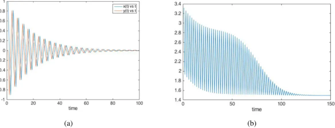
im-ply causation. Our definition of information transfer also verifies this fact, as is illustrated by the following example. Consider the following linear system with additive zero mean unit variance i.i.d. Gaussian noise.
x(t+ 1) =.5x(t) +ξx(t)
y(t+ 1) =.3x(t) +.7y(t) +ξy(t)
time 0 20 40 60 80 100 -0.03 -0.02 -0.01 0 0.01 0.02 0.03 0.04 x(t) y(t) time 0 20 40 60 80 100 0 0.1 0.2 0.3 0.4 0.5 0.6 Tx!y Ty!x
Figure 3.1 (a) The states are highly correlated. (b) The information transfer between the states.
As can be seen from fig8(a), the statesxandyare highly correlated, but from the system dynamics (3.8), the state ydoes not affect the dynamics ofxand so, intuitively,y should not causex. This is reflected in fig.8(b), where we find that the information transfer fromytoxis zero, whereas, sincex
affectsy, the transfer fromxtoyis non-zero.
The above example allows us to believe that our formalism of information transfer can be used to infer about the causal structure in a dynamical system. In later chapters, we will see, when directed in-formation and transfer entropy gives counter-intuitive results about the causal structure in a dynamical system, how our formalism gives the correct information about the causal structure.
3.1.1 Information Transfer and Causal Inference in Nonlinear Systems
In this subsection, we connect information transfer and causal inference for general nonlinear systems. However, we will consider systems without noise. In particular, we consider the system
whereS:Rn→Rnis assumed to be at least continuous andz(t)∈Rn. In component form, equation (3.9) can be written as zt+11 =S1(zt1, zt2,· · · , ztn) zt+12 =S2(zt1, zt2,· · · , ztn) .. . zt+1n =Sn(zt1, z2t,· · ·, ztn) (3.10)
Information transfer between the states of a dynamical system is defined in terms of difference of certain entropies, as the dynamical system evolves in time. As such to compute the information transfer, it is necessary to know the evolution of densities. This is given by the Perron-Frobenius (PF) operator P:L1(Rn)→ L1(Rn) (3.11) and is defined as Z ω Pρ(z)dz= Z S−1(ω) ρ(z)dz (3.12)
for anyω ∈ B(Rn), whereB(Rn)is the Borelσ-algebra onRn. WhenS is non-singular and
invert-ible, the PF operator can be written explicitly as
Pρ(z) =ρ[S−1(z)]|J−1| (3.13)
whereJis the Jacobian ofSand| · |signify the determinant. The joint densityρ(z)is used to define the Shannon entropy
H(z) =−
Z
Ω
ρ(z) logρ(z)dz (3.14)
whereΩis the sample space.
Assumption 9. We assumeΩto be Cartesian product ofΩ1,Ω2,· · · ,Ωn, in whichz1, z2,· · · , znare
respectively lying. Here eachΩiare open inR, fori= 1,2,· · · , n.
The marginal entropy of any variable of interest, sayz1is defined as H(z1) =−
Z
Ω1
whereρ1 = ρ(z1) = R
Ω2nρ(z)dz
2dz3· · ·dzn is the marginal distribution ofz1. Here we use the
notation
Ωjn= Ωj ×Ωj+1× · · · ×Ωn, 1≤j≤n, andΩ1n= Ω. (3.16)
We further use the notation
ρ6i =ρ(z1,· · ·zi−1, zi+1,· · · , zn) = Z Ωi ρ(z1,· · ·zi−1, zi+1,· · ·, zn)dzi ρ6i6j =ρ(z1,· · ·zi−1, zi+1,· · · , zj−1, zj+1· · · , zn) = Z Ωi×Ωj ρ(z1,· · ·zi−1, zi+1,· · ·, zj−1, zj+1,· · · , zn)dzidzj
With this, we state the following theorem which connects information transfer with causal infer-ence.
Theorem 10. IfSj is independent ofzi, thenTzi→zj = 0. At the same time,Tzi→zj need not be zero ifSjdoes not rely onzi.
Proof. Without loss of generality, we assume i = 2andj = 1, so that we look at the information transfer from z2 toz1. We consider the systemzt+1 = S(zt)given in component form as in (3.10).
Definezˆti=zt+1i and consider the dynamical system
zit+1 =Si(z)
ˆ
zit+1 =Si(ˆz)
(3.17)
fori= 1,2,· · · , n. Now, from (3.5),
Tz2→z1 = H(z1t+1, zt1)−H6z2(z1t+1, zt1)
= H(z1t+1,zˆt+11 )−H6z2(z
1
t+1,zˆt+11 ) (3.18)
It is given thatS1(z) is independent ofz2. Hence,S1(ˆz)is independent of zˆ2 and also z2. To
prove that ifS1(z)is independent ofz2, thenTz2→z1 = 0, we have to show
H(zt+11 ,zˆ1t+1) =H6z2(z
1
LetU be the sample space where the system (3.17) evolves. Note thatU satisfies assumption (9) and we use the notation defined in (3.16). For notational convenience we use the notationx1tto signify the subspace(zt1,zˆt1)>,x2t = zt2,yt = ˆz2t, xit = (zit,zˆti)> fori= 3,· · · , n. Similarly we defineUi
andUy. Hence we need to prove
H(x1t+1) =H6x2(x
1 t+1)
The dynamical system (3.17) can be written as
xit+1=φi(xt, yt) x2t+1=φ2(xt, yt) yt+1 =φy(xt, yt)
(3.19)
fori= 1,3,· · · , nandφi = (Si, Si)>,φ2 =S2andφy =S2. DefineΦ =
φ>i φ2 φy >
. For any subset ofU˜1,u˜1∈U˜1, we have
Z ˜ u1 (Pρ6x2)1(x1)dx1 = Z ˜ u1×U3n×Uy (Pρ6x2)(x 1, y, x3,· · · , xn) ×dx1dx3· · ·dxndy = Z Φ−621(˜u1×U3n×Uy) ρ6x2(x 1, y, x3,· · · , xn) ×dx1dx3· · ·dxndy Now1, Φ62−1(˜u1×U3n×Uy) = Φ1−621u˜1×U3n×Uy (3.20) Hence, Z ˜ u1 (Pρ6x2)1(x1)dx1 = Z Φ−1621u˜1 dx1· Z U3n×Uy ρ6x2(x1, x3,· · · , xn, y) ×dx1dx3· · ·dxndy = Z Φ−1621u˜1 ρ1(x1)dx1 = Z φ1−1˜u1 ρ1(x1)dx1 1 In the proof,Φ−1
where the last equality follows from the fact thatφ1and henceφ−11is independent ofx2. Again, Z ˜ u1 (Pρ)1(x1)dx1 = Z ˜ u1×U2n×Uy Pρ(x, y)dxdy = Z Φ−1(˜u 1×U2n×Uy) ρ(x, y)dxdy = Z φ−1u˜ 1×U2n×Uy ρ(x, y)dxdy = Z φ−11u˜1 dx1 Z U2n×Uy ρ(x)dx2· · ·dxndy = Z φ−11u˜1 ρ1(x1)dx1. Hence, Z ˜ u1 (Pρ6x2)1(x1)dx1 = Z ˜ u1 (Pρ)1(x1)dx1 (3.21)
for anyu˜1 ∈U1. Hence,(Pρ6x2)1 = (Pρ)1almost everywhere, whenφ1is independent ofx2. Now, in (15) it was shown that
H6x2(x1t+1) = − Z U (Pρ6x2)1(y1) log((Pρ6x2)1(y1)) ·ρ(x2|x1, x3· · · , xn, y) ·ρ3···n,y(x3,· · ·xn, y)dy1dx2dx3· · ·dxndy = − Z U (Pρ)1(y1) log((Pρ)1(y1)) ·ρ(x2|x1, x3· · · , xn, y) ·ρ3···n,y(x3,· · ·xn, y)dy1dx2dx3· · ·dxndy = − Z U1 (Pρ)1(y1) log((Pρ)1(y1))dy1 ·h Z U2 Z U3n×Uy ρ(x2|x1, x3· · · , xn, y) ·ρ3···n,y(x3,· · ·xn, y)dx2dx3· · ·dxndy i = − Z U1 (Pρ)1(y1) log((Pρ)1(y1))dy1 = H(x1t+1)
This is because the integrand in the brackets integrate to one. Hence,H(x1t+1) =H6x2(x1t+1), that is,
Hence,Tz2→z1 = 0.
3.2 n-step Information Transfer
The information transfer defined in definition (6) gives the information transferred fromxtoyas the dynamical system evolves from time steptto time stept+ 1. So one can look at this definition as aone-step transfer. However, it may happen thatx1does not affectx2 in one time step, but affects it
in two time steps. For, example, consider the linear system described by the graph given in figure3.2.
1 3 0 0 0 1 0 0 0 1 0 A = 2
Figure 3.2 A system where two step transfer is non-zero
Here the one step information transfer fromx1 tox3 is zero becausex1 does not affect the
dy-namics ofx3in one time step. Butx3, at the second time step, is affected byx1 and this should lead
to a non-zero transfer. This is what we call indirect transfer.
We propose a natural generalization of the definition of one step information transfer ton step transfer. Thenstep transfer fromxtoyis defined as transfer fromxtoyas the system evolves from time steptto time stept+nforn >0. To define thenstep transfer we introduce following notation
ytt+n= (y(t+n), y(t+n−1), . . . , y(t)).
Thenstep transfer is defined as follows :
Definition 11. [n-step Transfer] The information transferred over n > 0 time steps from x toy, denoted as[Tx→y]t+nt , as the dynamical system (3.1) evolves from time stepttot+nis defined as
[Tx→y]t+nt =H(ρ(y(t+n)|yt+n −1 t )−H(ρ6xtt+n−1(y(t+n)|y t+n−1 t ) whereρ6xt+n−1
t (·) is the notation that is used to signify the fact that dynamics inx component is freezed over the time period fromttot+n−1.
Using the proposed definition ofn-step transfer to the system of Fig. 3.2, we have the two step information transfer fromx1 tox3to be non zero. This is in accordance with the intuition that since x1 affectsx3 in the second time step, the information transfer in two time step should be non-zero.
With this definition ofn-step transfer, we have [Tx→y]t+2t = H(ρ(y(t+ 2)|y t+1 t )−H(ρ6xtt+1(y(t+ 2)|y t+1 t ) = H(ρ(ytt+2))−H(ρ6xt+1 t (y t+2 t ))−[Tx→y]t+1t
where we have used the fact that
[Tx→y]t+1t =H(ρ(y t+1 t ))−H(ρ6xt(y t+1 t )) Hence, [Tx→y]t+2t + [Tx→y]t+1t =H(ρ(y t+2 t ))−H(ρ6xtt+1(y t+2 t )) (3.22)
Equation (3.22), says that the total change in entropy, due to x, of the joint distribution of (y(t+ 2)y(t+ 1)y(t)), as the system (3.1) evolves from time steptto time stept+ 2, is equal to the sum of the information transfers fromxtoyover one time step and two time steps. In general, we have the following Theorem 12. n X i=1 [Tx→y]t+it =H(ρ(y t+n t ))−H(ρ6xtt+n−1(y t+n t ))
Proof. We prove this by induction. We saw that this is true fori = 1,2. Let this be true fori= k. Now, [Tx→y]t+k+1t =H(ρ(y(t+k+ 1)|ytt+k)) −H(ρ6xt+k t (y(t+k+ 1) |ytt+k)) = H(ρ(yt+k+1t ))−H(ρ6xt+k t (y t+k+1 t )) − H(ρ(yt+kt ))−H(ρ6xt+k−1 t (y t+k t )) = H(ρ(yt+k+1t ))−H(ρ6xt+k t (y t+k+1 t )) − k X i=1 [Tx→y]t+it
Hence, k+1 X i=1 [Tx→y]t+it =H(ρ(yt+k+1t ))−H(ρ6xtt+k(y t+k+1 t ))
Hence the proof.
We provide following definition of average information transfer.
Definition 13. [Average Information Transfer] We define the average information transfer fromxto
yas ¯ Tx→y = lim n→∞ 1 n n X i=1 [Tx→y]i0 (3.23) Lemma 14. We have ¯ Tx→y = ¯H(Y)−H¯6x(Y)
whereH¯(Y) = limn→∞ n1H(ρ(yn0))is the entropy rate ofyandH¯6x(Y) = limn→∞n1H(ρ6x(y0n))is
the entropy rate ofy, whenxis held frozen.
Proof. The proof follows directly from the definition of average information and theorem (12).
Though our concept of information transfer is way different than directed information, we will see later (chapter 4) that the average information transfer is indeed related to the average directed information.
3.3 Information Transfer and Dynamics of Linear Systems
A linear system may not exhibit the various complex dynamics that a nonlinear system can have, but still, the time domain trajectories of a linear system show different behaviours. The different behaviours that a linear system exhibit is governed by the eigenvalues of the system matrix. For example, if the eigenvalues of a linear discrete time system are outside the unit circle in the complex plane, then the trajectories diverge to infinity. Again, if they are on the unit circle, then the trajectories
oscillate. Similarly, if the eigenvalues are inside the unit circle, then the trajectories are stable, but depending on whether the eigenvalues are complex or real, the trajectories oscillate before settling down or does not oscillate. So one may think that the transient information transfer between the states should also show similar trends, depending on the location of the eigenvalues. In this section, we show, via simulations, that the transient one step information transfer in a linear system does show similar trends.
Case I : System is stable with real eigenvalues. We consider a two dimensional linear system
x(t+ 1) y(t+ 1) = 0 0.4 0.4 0 x(t) y(t)
In this case, the eigenvalues are real and are inside the unit circle. Hence, the trajectories does not show any oscillations and this is shown in fig.3.3(a).
(a) (b)
Figure 3.3 (a) Trajectories of the system. (b) IT fromxtoy.
The information transfer fromxtoyis shown in fig. 3.3(b). From the trajectory plot, we see that the trajectories show no oscillations and as expected, the transient information transfer also show no oscillation in the transients.
We consider a two dimensional linear system x(t+ 1) y(t+ 1) = 0 1 −0.952 0 x(t) y(t)
In this case, the eigenvalues are imaginary and are inside the unit circle. Hence, the trajectories initially show oscillations and then settle to the steady state value. This is shown in fig.3.4(a).
(a) (b)
Figure 3.4 (a) Trajectories of the system. (b) IT fromxtoy.
The information transfer from xto y is shown in fig. 3.4(b). From the trajectory plot, we see that the trajectories show oscillations and as expected, the transient information transfer also shows oscillation in the transients and then settles to the steady state value.
Case III : System is oscillatory.
Next consider a two dimensional linear system
x(t+ 1) y(t+ 1) = 0 1 −1 0 x(t) y(t)
In this case, the eigenvalues are on the unit circle. Hence, the trajectories oscillates and this is shown in fig.3.5(a).
From the trajectory plot, we see that the trajectories oscillate with constant amplitude and so does the transient information transfer, which is shown in fig.3.5(b).
(a) (b)
Figure 3.5 (a) Trajectories of the system. (b) IT fromxtoy.
We consider a two dimensional linear system
x(t+ 1) y(t+ 1) = 0 1 −1.012 0 x(t) y(t)
In this case, the eigenvalues are outside the unit circle and hence the system is unstable. The trajec-tories diverge to infinity and as the eigenvalues have imaginary part, the trajectrajec-tories oscillate as well. This is shown in fig.3.6(a) and the information transfer fromxtoyis shown in fig.3.6(b).
(a) (b)
Figure 3.6 (a) Trajectories of the system. (b) IT fromxtoy.
In this case also, we find that the trajectories and the information transfer follow similar patterns. So it is not wrong to believe that the information transfer does throw light on the nature of dynamics
exhibited by a dynamical system. So one can use the information transfer to infer about the dynamics of a nonlinear system also and this is addressed in the next section.
3.4 Set Oriented Method for Computation of Information Transfer
The definition of information transfer between the states is based on the evolution of the prob-ability density of the states and hence it is governed by the Perron-Frobenius operator. As we are going to see in a later chapter, in case of linear systems with additive Gaussian noise, the linearity property allows us to derive analytic expressions for the information transfer between the states. But for general discrete time maps, it is not possible to derive analytic closed form expressions for the information transfer. In fact, even in absence of noise, often it is difficult to derive an expression for the Perron-Frobenius operator and hence it will be difficult to obtain the information transfer. So, one has to look for numerical methods to compute the information transfer. In this section, we will describe set oriented numerical methods for finding the information transfer.
In order to obtain a finite-dimensional approximation of the continuous P-F operator, one consid-ers a finite partition of the state spaceXas follows :
X ={D1, D2, . . . , DL} (3.24)
such thatX = ∪L
i=1Di andDi ∩Dj = φfor alli 6= j. With this partition, the finite dimensional
approximation of the P-F semi-group is aL×LmatrixP such that
[P]ij =
m(f−1(Dj)∩Di) m(Di)
(3.25)
wheremis the Lebesgue measure. Theijthentry of the finite dimensionalP matrix gives the prob-ability of transition from cellDi to cellDj. Hence[P]ij =Prob(zt+1 ∈Dj|zt∈ Di). Moreover, if µz =
µz1 µz2 · · · µzL
is the density ofzat timet, then
µz0 =µzP (3.26)
In order to find the information transfer between the states in a system, we note that the one step information transfer from statexto stateycan be written as
[Tx→y]t+1t =H(ρ(y
0, y))−H
6
x(ρ(y0, y)). (3.27)
This is because H(ρ(y0|y)) = H(ρ(y0, y))−H(ρ(y)) and H(ρ(y)) = H6x(ρ(y)). We will use
equation (3.27) to compute the one step information transfer numerically.
Note that, the marginal distribution of(y0, y)can be obtained if one can compute the joint distri-butionρ(z0, z). Letµz be the distribution ofzat time stept. Hence,
Prob(z0 ∈Dj, z∈Di) =Prob(z∈Di).Prob(z0 ∈Dj|z∈Di) =µiz[P]ij (3.28)
So starting with an initial distributionµ0, using (3.26) and (3.28) one can calculate the joint probability
density of(z0, z), as the system evolves in time and thus one can calculate the marginal distribution
ρ(y0y). Letµy0ybe the distribution of the variable(y0, y), then
H(ρ(y0, y)) =−X[µy0y]ilog[µy0y]i (3.29)
Similarly, one can compute the entropy of(y0, y)whenxis held frozen and thus obtain the informa-tion transfer. Next, we illustrate this method of computainforma-tion of informainforma-tion transfer in two different systems, namely a linear system, where the information transfer can also be calculated analytically and a non-linear discrete time map.
Example 15(Linear system). Consider the linear system
xt+1=.9xt+ξx yt+1 = 10x+.5yt+ξy
(3.30)
From the system equations, we see that whilexenters the dynamics ofy,ydoes not affect the dynamics ofxand hence the information transfer fromxtoyshould be non-zero, whereas, the transfer fromy
toxshould be zero. In fact, in a later chapter, we prove the result for zero transfer for linear systems. Figure3.7(a) shows the information transfer from statexto statey, calculated using the set-oriented method and also using the formula for information transfer in a linear system. We find that though the values in the transients are not that close, as the system reaches steady state, the values of the
0 10 20 30 40 50 time -0.1 -0.05 0 0.05 0.1 0.15 0.2 Formula PF Operator (a) 0 10 20 30 40 50 time 0 0.05 0.1 0.15 0.2 0.25 0.3 0.35 (b)
Figure 3.7 (a) IT fromxtoy. (b) IT fromytox.
transfer match closely. Fig. 3.7(b) shows the information transfer fromytox. From the theory (we prove this result later) we know that the information transfer fromytoxshould be zero. This is shown by the plot obtained by using the formula for information transfer. The other plot shows the transfer obtained using the set-oriented methods and we find that thought the transfer is non-zero in the initial stages, it goes to zero as the system evolves and thus validating the use of set-oriented methods to calculate the information transfer. The value of the transfer, calculated using the set-oriented method depends on a number of factors like how the state space is discretized and how many initial points are chosen to obtain the finite dimensional P-F matrix. However, as the system evolves, these factors play less and less important roles and as the system approaches the steady state, the values of the transfer calculated using the set-oriented method approached the value obtained using the analytic expression of transfer.
Example 16(Henon map). In this example we consider the Henon map which is given by
x0 = 1 +y−ax2
y0=bx
(3.31)
witha, b >0.
For the first set of simulations, we choosea= 1.4andb=.3. This is when the Henon map exhibits chaotic behaviour and has a chaotic attractor, as shown in fig. 3.8(a). The corresponding invariant
-1.5 -1 -0.5 0 0.5 1 1.5 -0.5 -0.4 -0.3 -0.2 -0.1 0 0.1 0.2 0.3 0.4 0.5 (a) -1.5 -1 -0.5 0 0.5 1 1.5 -0.5 -0.4 -0.3 -0.2 -0.1 0 0.1 0.2 0.3 0.4 0.5 0 0.05 0.1 0.15 0.2 (b) 0 20 40 60 80 100 time 0.8 1 1.2 1.4 1.6 1.8 2 (c) 0 20 40 60 80 100 time -1.4 -1.2 -1 -0.8 -0.6 -0.4 -0.2 0 (d)
Figure 3.8 (a) Phase space trajectories (b) Invariant measure. (c) Information transfer fromx to
measure for the chosen set of parameters is shown in fig 3.8(b). The corresponding information transfers are shown in fig3.8(c) and fig3.8(d).
0 20 40 60 80 100 time 0 0.5 1 1.5 2 2.5 3 (a) 0 20 40 60 80 100 time -0.6 -0.5 -0.4 -0.3 -0.2 -0.1 0 0.1 0.2 0.3 0.4 (b)
Figure 3.9 (a) Information transfer fromxtoy. (b) Information transfer fromytox.
For the second set of simulations simulation purposes, we choosea=.18andb=.7. With these set of parameter values, the Henon map has a periodic orbit. Figure3.9(a) shows the information transfer fromxtoy and fig. 3.9(b) shows the information transfer fromytox. Before reaching the steady state, from the information transfer plots, it is clear thatx has a greater influence ony than whatyhas onx. Moreover, the information transfer oscillates and this is because of the presence of the periodic orbit.
Example 17 (Van der Pol Oscillator). Van der Pol oscillator is a non-conservative system with a
non-linear damping and it evolves in time according to the second order differential equation
¨
x−µ(1−x2) ˙x+x= 0 (3.32)
where x is the position and µis a scalar indicating the nonlinearity and the strength of damping. Using the variabley = ˙x, the system equations can be written as
˙ x=y
˙
y =µ(1−x2)y−x
Whenµ= 0, there is no damping and so the equation of motion becomes
¨