Rise and Fall Patterns of Information Diffusion:
Model and Implications
Yasuko Matsubara
Kyoto University y.matsubara@ db.soc.i.kyoto-u.ac.jpYasushi Sakurai
NTT Communication Science Labs [email protected]B. Aditya Prakash
Carnegie Mellon UniversityLei Li
University of California, Berkeley [email protected]
Christos Faloutsos
Carnegie Mellon UniversityABSTRACT
The recent explosion in the adoption of search engines and new media such as blogs and Twitter have facilitated faster propagation of news and rumors. How quickly does a piece of news spread over these media? How does its popular-ity diminish over time? Does the rising and falling pattern follow a simple universal law?
In this paper, we proposeSpikeM, a concise yet flexible analytical model for the rise and fall patterns of influence propagation. Our model has the following advantages: (a) unification power: it generalizes and explains earlier theo-retical models and empirical observations; (b) practicality: it matches the observed behavior of diverse sets of real data; (c) parsimony: it requires only a handful of parameters; and (d) usefulness: it enables further analytics tasks such as fore-casting, spotting anomalies, and interpretation by reverse-engineering the system parameters of interest (e.g. quality of news, count of interested bloggers, etc.).
Using SpikeM, we analyzed 7.2GB of real data, most of which were collected from the public domain. We have shown that our SpikeM model accurately and succinctly describes all the patterns of the rise-and-fall spikes in these real datasets.
Categories and Subject Descriptors: H.2.8 [Database management]: Database applications–Data mining General Terms: Algorithms, Experimentation, Theory Keywords: Information diffusion, Social networks
1.
INTRODUCTION
How do spikes behave in social media? Online social me-dia is spreading news and rumors in new ways and search en-gines have facilitated such spreading magnificently, creating bursts and spikes. Some rumors (or memes, hashtags) start
Permission to make digital or hard copies of all or part of this work for personal or classroom use is granted without fee provided that copies are not made or distributed for profit or commercial advantage and that copies bear this notice and the full citation on the first page. To copy otherwise, to republish, to post on servers or to redistribute to lists, requires prior specific permission and/or a fee.
KDD’12,August 12–16, 2012, Beijing, China.
Copyright 2012 ACM 978-1-4503-1462-6 /12/08 ...$15.00. 20 40 60 80 100 120 0 50 100 Time Value Original SpikeM 20 40 60 80 100 120 0 50 100 Time Value Original SpikeM
(a) Pattern C1 (b) Pattern C2
20 40 60 80 100 120 0 50 100 Time Value Original SpikeM 20 40 60 80 100 120 0 50 100 Time Value Original SpikeM (c) Pattern C3 (d) Pattern C4 20 40 60 80 100 120 0 50 100 Time Value Original SpikeM 20 40 60 80 100 120 0 50 100 Time Value Original SpikeM
(e) Pattern C5 (f) Pattern C6
Figure 1: Modeling power of SpikeM: six types of spikes (K-SC from [41]) shown as dots, and our model fit in solid red line. Data sequences span over 120 time-ticks, while SpikeM requires only seven pa-rameters. The fit is so good, that the red line is often invisible, due to occlusion.
slowly and linger; others spike early and then decay; others show more complicated behavior, as we show inFigure 1.
Do real rise-and-fall patterns have any qualitative differ-ences? Do they form different classes? If yes, how many? Earlier work on Youtube data claims there are four classes [6]. Empirical work found six classes [41]. How many classes are there after all?
Our answer is:one. We provide a unifying model,SpikeM, that requires only a handful of parameters, and we show that it can generate all patterns found in real data simply by changing the parameter values.
Figure 1 shows six representative spikes of online media
(memes) fromK-SC [41], as gray circles, as well as our fit-ted model, as a solid red line. Notice that the fitting is very
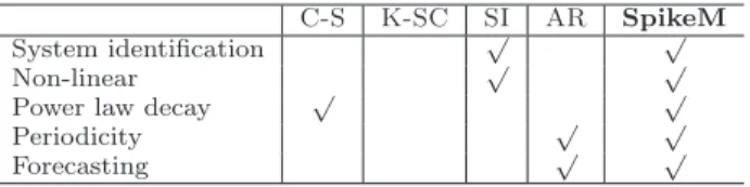
C-S K-SC SI AR SpikeM
System identification √ √
Non-linear √ √
Power law decay √ √
Periodicity √ √
Forecasting √ √
Table 1: Capabilities of approaches. Only our ap-proach meets all specs.
good, despite the fact that ourSpikeMmodel requires only seven parameters, and that the time-sequences span 120 in-tervals.
Informally, the problem we want to solve is to model/predict an activity (e.g., number of blog postings), as a function of time, given some breaking-news at a given timetick. We will use a blogger example for brevity and clarity, but many other processes could be also modeled (people buying prod-ucts, computer viruses infecting machines, rumors spreading over Twitter, etc). Thus, we have:
Informal Problem 1 (what-if). Givena network of bloggers (/hosts/buyers), a shock (e.g., event) at time nb,
the interest/quality of the event, the count Sb of bloggers
that immediately (= timenb) blog about the event,findhow
the blogging activity will evolve over time.
A closely related problem is to develop a parsimonious model, that can be made to fit several spikes observed in the past (as we do inFigure 1). That is,
Informal Problem 2 (model design). Giventhe be-havior of several spikes in the past,findan equation/model that can explain them, with as few parameters as possible. It would be good if the parameters had an intuitive explana-tion (like, ‘number of bloggers’, ‘quality of news’, etc, as op-posed to, say,a1,a2of an autoregressive model (AR/ARIMA)).
In this paper, we proposeSpikeMmodel to solve both of the aforementioned problems. OurSpikeMhas the follow-ing advantages:
• Unification power: it includes earlier patterns and models as special cases ([41,21]),
• Practicality: it matches the behavior of numerous, diverse, real datasets, including power-law decay
• Parsimony: our model requires only a handful of pa-rameters
• Usefulness: thanks to theSpikeMmodel, we can an-swer ‘what-if’ questions (seesubsection 5.1), spot out-liers, reverse-engineer the system parameters (quality of news, count of interested bloggers, time-of-day be-havior of bloggers)
OurSpikeM model is enabled by a careful design to in-corporate (a) the power-law decay in infectivity, (b) a finite population, and (c) proper periodicities. Earlier models ig-nored one or more of the above issues.
Thanks to thepracticalityof SpikeM, we can make fore-casting, analysis of ’what-if’ scenarios, and detection of anoma-lies, as we show insection 4andsection 5. We should high-light that traditional AR, ARIMA and related linear models are fundamentally unsuitable, because they arelinear(and can diverge to infinity) and because they lead to exponen-tial decays (as opposed to the power law that reality seems to obey). Table 1 illustrates the relative advantages of our method: the C-S method (Crane and Sornette) [6] assumes
an infinite population of bloggers; the clusters inK-SC[41] (repeated inFigure 1) are non-parametric and are incapable of forecasting. The SI model (closely related to the Bass model [3] of the market penetration of new products) leads to exponential decay, as opposed to the power-law decay that we observe in real data.
Outline
.
The rest of the paper goes as follows: Section2presents an overview of the related work and Section3the proposed model. Sections 4 and 5 show our experimental results on a variety of datasets. We conclude in section7.
2.
BACKGROUND
In this section, we present the fundamental concepts. Epidemiology fundamentals. The most basic epi-demic model is the so-called ‘Susceptible-Infected’ (SI) model. Each object/node is in one of two states - Susceptible (S) or Infected (I). Each infected node attempts to infect each of its neighbors independently with probability β, which reflects the strength of the virus. Once infected, each node stays infected forever. If we assume that the underlying network is a clique ofNnodes, and use our notation (‘B’ for blogged = infected) the most basic form of the model is:
dB(t)
dt = β∗(N−B(t))B(t) (1) where the time t is considered continuous, dB/dt is the derivative, and the initial condition reflects the external shock (say,B(0) =bexternally infected people). The justi-fication is as follows: βis the strength of the virus, that is, the probability that an encounter between an infected person (‘B’) and an uninfected one, will end up in an infection - and we haveB∗(N−B) such encounters. The solution forB() is the sigmoid, and its derivative is symmetric around the peak, with an exponential rise and an exponential fall (we discuss later inFigure 2). There we also show the weakness of the SI model: real data have a power-law ‘fall’ pattern.
Self-excited Hawkes process. Crane et al. [6] used a self-excited Hawkes conditional Poisson process [12] to model YouTube views per day, showing that spikes in the activity have a power-law rise pattern, and a power-law fall pattern, depending on the model parameters. Roughly, the Hawkes process is a Poisson process where the instantaneous rate is not constant, but depends on the count of previous events, whose effect drops with the ageτ of the event. That is, if there were a lot of events (viewings/bloggings) recently, we will have many such events today.
The base model states that the rate of spread of infec-tion depends on (a) the external source S(t) and (b) self-excitation, that is, on earlier-infected nodes (i = 1, . . .); these nodes spread the infection with decaying virus strength φ(τ), their age τ grows, times some constantµi. The
con-stantµiis equivalent to the degree of the infected nodei.
dB(t)
dt = S(t) +
X
i,ti≤t
µiφ(t−ti) (2)
The model typically assumes that the µi values are equal,
namely that all nodes have the same degree (‘homogeneous’ graph). It also silently assumes that there are infinite nodes available for infection, and it may actually diverge to infinity. Next we present our SpikeM model, which avoids the shortcomings of the SI and Hawkes models, and has several more desirable properties.
3.
PROPOSED METHOD
In this section we present our proposed method, analyze it, and we provide the reader with several interesting -at least in our opinion- observations.
Our model tries to capture the following behaviors, that we observed with several of our real data
• P1: power-law fall pattern
• P2: periodicities
and at the same time we want to
• P3: avoid the divergence to infinity
that other models may have. To handle P3 (divergence), we force our model to have a finite population, and adjust the equations accordingly. To handle P1 (power-law fall pat-tern), we assume that the infectivity of a node (= popularity of a blog post) decays with theinfluence exponent, which we set at -1.5. The handling of periodicities is discussed in
subsection 3.2.
We describe our model in steps, adding complexity, and we start with the base model.
Preliminaries
.
We assume there areNbloggers, and none of them is yet blogging about the topic of interest. At time nb, an event happens (such as the 2004 Indonesian tsunami,or a controversial political speech such as ‘lipstick on a pig’), andSbbloggers immediately blog about it. We refer to this
external event as ashock, andnbandSbare the birth-time
and the initial magnitude of the shock.
Our model needs a few more parameters: the first is the quality/interestingness of the news, which we refer to asβ, since this is the standard symbol for the infectivity of a virus in epidemiology literature. Ifβis zero, nobody cares about this specific piece of news; the higher the value, the more bloggers will blog about it.
Finally, we have the decay function f(n), which models how infective/influential a blog posting is, at agen. Stan-dard epidemiology models assume thatf() is constant (once sick, you have the same probability of infecting others); re-cent analysis has shown that the influence drops with age, following a power law.
The above are the parameters of the base model. Before we list the equations, we want to briefly mention a derived quantity, β∗N; this quantity roughly corresponds to the R0 (‘R-naught’) found in the epidemiology literature. This
tells us the size of the “first burst”: if only one person was infected, how many would be infected in the next time-tick?1
In summary, the scenario we model is as follows:
• nothing happens, until a news-event appears, at birth-timenb.
• Sbbloggers immediately blog about it.
• other bloggers visit the initialSb (or follow-up)
blog-gers, and occasionally get ‘infected’ and blog about the event, too.
We also assume that
• each blogger blogs at most once about the event
• no other related event occurs - that is, the shock func-tionS() has only one spike.
1
yes, it should beN−1, but we sacrifice accuracy, for intu-ition.
Without loss of generality, we also assume that once an un-informed blogger sees an infected/un-informed blog, he/she al-ways blogs about the event (if he/she blogs with probability ρ <1, we could absorbρin the infectivity factorβ)
Our goal is to find an equation to describe the number ∆B(n) of people blogging at time-tickn, as a function of n and of course the system parameters (total number of bloggersN, strength of infectionβetc).
3.1
Base model -
SpikeM-
BaseThe model we propose has nodes (=bloggers) of two states:
• U:Un-informed of the rumor
• B: informed, andBlogged about it
For those who just got informed at time-tick n, we’ll use the symbol ∆B(n), and we assume that, once informed, a person will blog about the rumor immediately.
Let U(n) be the number of un-informed people at time n, and let ∆B(n) the number of people that just found out about the rumor at timen, and blogged immediately about it.
Model 1 (SpikeM-Base). Our base model is governed by the equations ∆B(n+ 1) =U(n)· n X t=nb ∆B(t) +S(t) ·f(n+ 1−t) +ǫ (3) U(n+ 1) =U(n)−∆B(n+ 1) (4) where f(τ) =β∗τ−1.5 (5) and initial conditions:
∆B(0) = 0, U(0) =N
In addition, we add an external shockS(n), a spike generated at birth-timenb. Mathematically, it is defined as follows:
S(n) =
0 (n6=nb)
Sb (n=nb) (6)
Justification of the model
.
We do it in steps:• The term ∆B(t) +S(t) captures the count of bloggers plus external sources, that got activated at time-tick t; their infectivity is modulated by the f() infectiv-ity function, since we assume that the infectivinfectiv-ity of a source/blogger decays with time. The summation is over all past time-ticks since the birth-timenbof the
shock.
• The infectivity function f() exactly follows a power law with exponent -1.5 as discovered by earlier work on read data: real bloggers [22], and response to mails by Einstein and Darwin [2].
• The meaning of the summation is the available stim-uli at time-tick n; the available targets are the un-informed bloggers U(n), and the product gives the number of new infections.
• We add a noise termǫto handle cases such as hashtag ‘egypt’ on Twitter: some people tweet about Egypt anyway, but a large shock occurred during the events in Tahrir square. Very often,ǫ≃0.
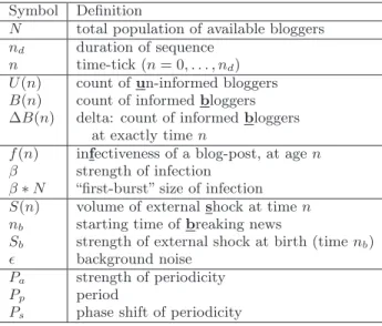
Symbol Definition
N total population of available bloggers nd duration of sequence
n time-tick (n= 0, . . . , nd)
U(n) count ofun-informed bloggers B(n) count of informedbloggers ∆B(n) delta: count of informedbloggers
at exactly timen
f(n) infectiveness of a blog-post, at agen β strength of infection
β∗N “first-burst” size of infection S(n) volume of externalshock at timen nb starting time ofbreaking news
Sb strength of external shock at birth (timenb)
ǫ background noise Pa strength of periodicity
Pp period
Ps phase shift of periodicity
Table 2: Symbols and definitions
This completes the justification of our base model.
We also mention some facts that our model obeys: by definition B(n) = n X t=0 ∆B(t) and of course we have the invariant
B(n) +U(n) =N
whereN is the total number of people/bloggers.
3.2
With periodicity -
SpikeMBloggers may modulate their activity following a daily cycle (or weekly, or yearly). For example, among theU(n) uninformed bloggers at timen, a fraction of them are not paying attention (say, because they are tired or asleep). How can we reflect this in our equations? We propose an answer below, and then we provide the justification.
Model 2 (SpikeM). We can capture the periodic be-havior of bloggers with the following equations:
∆B(n+ 1) =p(n+ 1)· U(n)· n X t=nb ∆B(t) +S(t) ·f(n+ 1−t) +ǫ (7) p(n) = 1−1 2Pa sin 2π Pp(n+Ps) + 1 (8)
whereU(n),S(t) andf(n) are defined in Model1.
Justification
.
The model is identical toSpikeM-base, with the addition of the periodicity factorp(·). This captures the fact that bloggers tone down their activity, say, during the night, or even stop it altogether. The idea is that U(·) is the count of victims available for infection, and the summa-tion is the number of attacks. Under normal circumstances, each victim-attack pair would lead to a new victim; however, since the victims are not paying full attention (tired/asleep), the attacks are not so successful, and thus we prorate them by thep() periodic function.30 40 50 60 70 80 90 100 110 120 0 50 100 Time Value SI spikeM Original
(a) Whole sequence (linear-logscale) duration=120, peak atnmode= 42
10 20 30 40 100 Time Value exponential 0 20 40 60 80 100 Time Value
(b) Rise-plot (linear-logscale) (c) Fall-plot (linear-log) Timen:42, 41, ... 1 Timen:42, 43, ...120 100 101 100 Time Value 100 101 100 Time Value power law
(d) Rise-plot (log-logscale) (e) Fall-plot (log-log) Timen:42, 41, ... 1 Timen:42, 43, ...120 Figure 2: Fitting results of SpikeM vs. SI for pat-tern C1 in Figure 1. The original sequence (in gray circles), and our model (red line) have an exponen-tial rise and a power-law drop; the SI model (blue dashed line) is exponential on both and thus unre-alistic. Top row: full interval; left column: only the rise part; right column: only the ‘fall’ part.
• Ppstands for the period of the cycle (say, 24 hours).
• Psstands for the phase shift: if the peak activity is at
noon, and the period isPp=24 hours, thenPs=18.
• Pa depends on the amplitude of the fluctuation, and
specifically it gives the relative value of the off-time (say, midnight), versus peak time (say, noon). Thus, ifPa=0, we have no fluctuation.
3.3
Additional details
Model extensions
.
We could easily extend our model so that it has several shocks as opposed to just one as consid-ered here. We could also extend it to have multiple cycles (daily, weekly, yearly). We do not elaborate on these ex-tensions for two reasons: (a) for clarity and (b) because the current model fits real data very well, anyway.Learning the parameters
.
Our model consists of a set of seven parameters: θ ={N, β, nb, Sb, ǫ, Pa, Ps}. Given areal time sequence X(n) of bloggers at time-tick n (n = 1, . . . , nd), we use Levenberg-Marquardt (LM)[23] to
min-imize the sum of the errors: D(X,θ) = Pnd
n=1(X(n)−
∆B(n))2
.
Analysis - exponential rise, power-law fall
.
It is not obvious from the equations of our model, but its rise pat-tern is exponential, while the fall patpat-tern obeys a power law. This is desirable, because this behavior seem to be prevailing in real data, as we show inFigure 2. Letnmodedenote the time-tick at which the wave ∆B() reached its maximum volume. By rise plot we mean the plot of
val-ues from the birth-timenb untilnmode (and reversing time
abs(n−nmode)) The fall-plot is defined similarly: activity
∆B() versus delay from the peak n−nmode. Notice that
there is a power law for the fall, and an exponential shape for the rise. We also show the traditional ‘SI’ model, which, as expected, exhibits exponential behavior for both rise and fall.
4.
EXPERIMENTS
To evaluate the effectiveness of SpikeM, we carried out experiments on real datasets. The experiments were de-signed to answer the following questions:
• Q1: Can we explain the cluster centers of K-SC?
• Q2: How well do we matchMemeTrackerdata?
• Q3: How does it compare with other data?
• Q4: How well do we forecast future patterns? Dataset description
.
We performed experiments on the following three real datasets.• MemeTracker: This dataset covers three months of blog activity from August 1 to October 31 20082
, It contains short quoted textual phrases (“memes”), each of which consists of the number of mentions over time. We choose 1,000 phrases in blogs with the highest vol-ume in a 7-day window around their peak volvol-ume.
• Twitter: We used more than 7 million Twitter3
posts covering an 8-month period from June 2011 to January 2012. We selected the 10,000 most frequently used hashtags.
• GoogleTrends: This dataset consists of the volume of searches for various queries (i.e., words) on Google4
. Each query represents the search volumes that are re-lated to keywords over time.
4.1
Q1: Explaining
K-SCclusters
The results on this dataset were already presented insection 1
(see Figure 1). Our model correctly captures the six
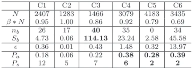
pat-terns of K-SC. Table 3 gives a further description of the SpikeM fitting. Our model consists of seven parameters, each of which describes the behavior of spikes. Note that the total populationsNare almost the same for all patterns, (around 2,000 to 3,000). This is because these six patterns are scaled on they-axis so that they all have a peak volume of 100. We can see thatβ∗N is between 0.7−1.0 for these six patterns. We also see that Pattern C3 has an extreme shock Sb = 114 at time nb = 40, which means that this
spike is strongly affected by the external burst of activity
(seeFigure 1(c)). On the other hand, Patterns C4-C6 have
several peaks about 24 hours apart with a strengthPa≃0.4.
We also evaluated our fitting accuracy by using the root mean square error (RM SE) between estimated values and real values: RM SE = q1
nd Pnd
n (X(n)−∆B(n))
2. Table 4
shows the fitting accuracy result for six patterns of K-SC. We comparedSpikeMwithSImodel. As discussed insection 3
(seeFigure 2),SIcannot model the tail parts of the spikes.
On the other hand, our solution,SpikeMachieves high ac-curacy for every pattern ofK-SC.
2 http://memetracker.org/ 3 http://twitter.com/ 4 http://www.google.com/insights/search/ C1 C2 C3 C4 C5 C6 N 2407 1283 1466 3079 4183 3435 β∗N 0.95 1.00 0.86 0.92 0.79 0.69 nb 26 17 40 35 0 34 Sb 4.73 0.06 114.13 23.24 2.58 45.58 ǫ 0.36 0.01 0.43 1.48 0.32 13.97 Pa 0.18 0.06 0.22 0.38 0.28 0.39 Ps 12 5 7 6 2 2
Table 3: The model parameters of our SpikeM best fitting on six patterns of K-SC (see Figure 1).
Pattern C1 C2 C3 C4 C5 C6
SpikeM 1.84 1.61 0.97 4.08 3.33 5.89
SI 15.64 6.78 19.65 25.29 20.36 21.76
Table 4: Fitting accuracy of SI vs. SpikeM on six patterns of K-SC. SpikeM consistently outperforms SI with respect to accuracy (RM SE) between the original values and the models.
4.2
Q2: Matching
MemeTrackerpatterns
Figure 3shows the results of model fitting on the
Meme-Trackerdataset. We selected six typical sequences according to the K-SC clusters. That is, each sequence corresponds to each pattern (C1-C6). We show the original sequences (black dots) andSpikeM fitting, ∆B(n) (red line) in both linear-linear (top) and log (bottom) scales. In the log-log scale, we also show the count of un-informed blog-loggers, U(n). InFigure 3, the bottom table shows the short phrases (memes) of each sequence. All of the phrases are sourced from U.S. politics in 2008. We obtained several observations for each sequence:
• Patterns C1 and C2: almost the same size of popu-lation, N ≃ 500, except that C2 has a quicker rise and fall (i.e., stronger infection,β∗N = 1.4) than C1 (β∗N= 0.94).
• Pattern C3: this sequence has a sudden rise and a power law decay. There is a slight daily periodicity.
• Patterns C4 and C5: there are clearly daily periodic-ities. Pattern C6, “lipstick on a pig” has the largest population of all six sequences (i.e.,N = 6259).
• Pattern C6: the sequence: “yes we can” consists of huge spikes around n = 40, and constant periodic noise. This is because the bloggers mention this phrase as Barack Obama’s slogan as well as with more gen-eral meanings. We can also find that there are sevgen-eral extreme points (i.e., missing values) aroundn = 120 (see blue circle in log-log scale).
4.3
Q3: Matching other data
We also demonstrate the effectiveness of our model for other types of spikes.
Fitting on Twitter data. Figure4describes our fit-ting results on thehashtags ofTwitterdata. In this figure, we can see that Twitter data behave similarly to Meme-Trackerdata. Due to space limitations, we show only three major hashtags. Note that the top and bottom rows are in linear-linear and log-log scales, respectively. Our model captures the following characteristics: (a) #assange: this is a topic about Julian Assange, the founder of WikiLeaks. There are several mentions before the peak point (December 5, 2011). (b) #stevejobs: there is a sudden peak on
Octo-50 100 150 0 20 40 60 Time Value N =562, beta*N=0.94 ∆ B(n) Original 50 100 150 0 50 100 Time Value N =405, beta*N=1.42 ∆ B(n) Original 50 100 150 0 100 200 300 400 Time Value N =3529, beta*N=0.81 ∆ B(n) Original 102 100 101 102 103 Time Value N =562, beta*N=0.94 ∆ B(n) U(n) Original 101 102 100 101 102 103 Time Value N =405, beta*N=1.42 ∆ B(n) U(n) Original 102 100 102 104 Time Value N =3529, beta*N=0.81 ∆ B(n) U(n) Original
(a) Pattern C1: Meme #109 (b) Pattern C2: Meme #34 (c) Pattern C3: Meme #13
50 100 150 0 20 40 60 80 Time Value N =772, beta*N=1.04 B(n) Original 50 100 150 0 50 100 150 200 Time Value N =6259, beta*N=0.73 ∆ B(n) Original 50 100 150 0 50 100 150 Time Value N =3234, beta*N=0.69 ∆ B(n) Original 102 100 102 Time Value N =772, beta*N=1.04 ∆ B(n) U(n) Original 102 100 102 104 Time Value N =6259, beta*N=0.73 ∆ B(n) U(n) Original 102 100 102 104 Time Value N =3234, beta*N=0.69 ∆ B(n) U(n) Original
(d) Pattern C4: Meme #87 (e) Pattern C5: Meme #9 (f) Pattern C6: Meme #3
#109 the most serious financial crisis since the great depression #87 what is required of us now is a new era of responsibility #34 i love this country too much to let them take over another election #9 you can put lipstick on a pig
#13 hope over fear, unity of purpose over conflict and discord #3 yes we can yes we can
Figure 3: Results of SpikeM fitting on six patterns from MemeTracker dataset. The figures show in both ‘linear-linear’(top) and ‘log-log’(bottom) scales. The bottom table lists the phrase (“meme”) of each patterns.
50 100 150 0 50 100 Time Value N =992, beta*N=1.41 ∆ B(n) Original 50 100 150 0 500 1000 1500 Time Value N =6475, beta*N=2.00 ∆ B(n) Original 50 100 150 0 50 100 150 Time Value N =1266, beta*N=1.41 ∆ B(n) Original 101 102 100 102 Time Value N =992, beta*N=1.41 ∆ B(n) U(n) Original 102 100 102 104 Time Value N =6475, beta*N=2.00 ∆ B(n) U(n) Original 102 100 102 104 Time Value N =1266, beta*N=1.41 ∆ B(n) U(n) Original
(a) #assange (b) #stevejobs (c) #arresteddevelopment
Figure 4: Results of SpikeM fitting on three hashtags fromTwitterdataset. The top and bottom rows show in linear-linear scale, and log-log scale, respectively.
20 40 60 0 50 100 Time Value Original SpikeM 10 20 30 40 50 0 50 100 Time Value
(a) “tsunami” (2005) (b) “Harry Potter” (2007) Figure 5: SpikeM fitting on GoogleTrends dataset: the volume of searches for the keyword (in black dots) and fitting results (in red lines). Note that the window size is per week.
ber 5, 2011, with a long heavy tail (see Figure4(b) in log-log scale). This was caused by the death of Steve Jobs. (c) #ar-resteddevelopment: this a topic about the movie “Arrested Development”. There is a clear daily periodicity with a peak point.
Fitting on GoogleTrend data. We can also observe influence propagation in queries on internet search engines. Figure5shows two different types of spikes onGoogleTrends. For an external catastrophic event (a) “tsunami”, we see that there is a super quick rise immediately after the Indian Ocean earthquake and tsunami in 2005. In contrast, (b) “harry potter” has a slower rise, which is because this spike was generated by “word-of-mouth” activity surrounding the release of a Harry Potter movie in 2007. SpikeMevidently captures both types of spikes successfully.
4.4
Q4: Tail-part forecasts
So far we have seen how SpikeM captures the pattern dynamics for various spikes. Here, we answer a more prac-tical question: given the first part of the spike, how can we forecast the future behavior of the tail part? Figure6shows results of our forecasts onMemeTrackerdata. We selected two the highest population phrases (#9 and #13 in Fig-ure3). We trained our models by using the values obtained over a period of 54 hours (solid black lines in the figure), and then forecasted the following days (solid red lines, about five days). Note that the vertical axis uses a logarithmic scale. We comparedSpikeMwith the auto regressive model (AR). For a fair comparison, we used seven regression coefficients, which was the same size as our model parameters.
Our method achieves high forecasting accuracy whileAR failed to forecast future patterns. More specifically, the re-construction errors of SpikeMare RM SE= 9.26 and 8.93 for #9 and #13, while ARhas errors of 13.98 and 14.19. Similar trends are observed in other phrases, however we omit the results due to space limitations. More importantly, our model can forecast the rise part of spikes as well as the tail part (discussed in Section5).
5.
DISCUSSION -
SpikeMAT WORK
Our proposed model,SpikeMis capable of various appli-cations. Here, we describe important applications and show some usefulness examples of our approach.
5.1
“What-if” forecasting
We have discussed tail-part forecasting insubsection 4.4. Ideally, we want to forecast not only the tail-part, but also the rise-part of a spike. This is much more difficult, because we usually have very few points in the rise-part of a spike.
0 50 100 150 100
102
Time (per hour)
Value N =5960, beta*N=0.7 spikeM AR Original 0 50 100 150 100 102
Time (per hour)
Value
N =3481, beta*N=1.2 spikeM AR Original
(a) Meme #9 (b) Meme #13
Figure 6: Results of tail-part forecasting on Meme-Tracker data. We train spikes fromn= 0 to 54, and then, start forecasting at time n= 54. Our SpikeM reflects reality better, while AR quickly converges to the zero.
However, if this is a repeating event, like, say, the spikes induced by ‘Harry Potter’ movies releases, can we forecast future spikes if we know the release date of the next movie? It turns out that ourSpikeMmodel can help with this (dif-ficult) task, too.
Thus, the problem we address in Figure7 is as follows: we are given (a) the first spike in 2009, “Harry Potter and the Half-Blood Prince” (n = 185); (b) the release dates of the two sequel movies (blue text with as arrows pointed at n = 255 and 289), and (c) the access volume before the release dates (and specifically from 8 to 2 weeks before). Can we forecast the rise and fall shapes of upcoming spikes and their peak points?
Solution and results. SpikeM can predict the po-tential populationN of users who are interested in “Harry Potter”, and the strength of ‘word-of-mouth’ infection: β. Our solution is to assume that these values are fixed for all of the sequel spikes. The only difference is the strength of the “external shock”, i.e.,nb andSb. Our solution consists
of the following three-step process:
1. Train the parameter setθby using the first spike (solid black line in the figure).
2. With the fixed parameters θ, infer the new values of
˜
nband ˜Sbby using the beginning part of the next spike
(blue lines between double arrows atn= 250 and 280). 3. Generate the spikes usingθand ˜nband ˜Sb(red lines).
In conclusion, Figure 7 shows that our model successfully captures the two sequel spikes and peak pointsnmode.
5.2
Outlier detection
Since SpikeM has a very high fitting accuracy on real datasets (described in section 4), another natural applica-tion would be anomaly detecapplica-tion. Figure 8shows the fitting result of Figure 5 (a), in a log-log scale. Note that the black circles are the original sequence, and the pink line is our model fitting. We can visually observe that there are several points that do not overlap the model. For example, (a) on March 29, there is one spike, since another earth-quake occurred on March 28. (b) There is a huge spike on December 26, 2005, which is exactly one year after the In-dian Ocean earthquake.
5.3
Reverse engineering
Most importantly, our model can provide an intuitive ex-planation such as the potential number of interested
blog-150 200 250 300 0 20 40 60 80
Time (per week)
Value July 15, 2009
"Harry Potter and the Half-Blood Prince"
November 19 , 2010
"Deathly Hallows part 1" July 15, 2011 "Deathly Hallows part 2"
Figure 7: Results of “what-if ” forecasting for the Harry Pot-ter series. We trained paramePot-ters by using (a) the first spike around July 15, 2009 (black solid line), and (b) access volume two months before the release (blue lines with double arrows around time n = 250, 280) and then, forecasted the following two spikes (red lines).
100 101 101
102
Time (per week)
Value Dec. 26 Indian Ocean earthquake Mar. 29 Scientists puzzled no tsunami
after quake Dec. 26 World marks
tsunami anniversary
Figure 8: Outlier detection on Google-Trends dataset (in log-log scale). No-tice that the biggest spike, “world marks tsunami anniversary” occurred after one year (i.e., 52 weeks later).
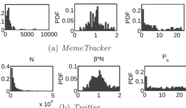
gers, and the quality of news. Here we report our discoveries onMemeTrackerandTwitterdatasets (see Figure9).
Observation 1 (Total population of bloggers). The total populations of potential bloggers/usersN are al-most same for both datasets (aroundN= 1,000−2,000).
We also note that they are skewed to the right, i.e., there is a long tail of larger values.
Observation 2 (Strength of first infection). The strength of the “first burst” isβ∗N≃1.0for each dataset.
The above two observations agree with the intuition: we can see common behavior for MemeTracker and Twitter, which means that they have similar characteristics in terms of social activities.
Observation 3 (Common activity and periodicity). Typical user behavior is to have a daily periodicity with (a) phase shiftPs= 0 (small population during early morning,
large population at peak point, 6pm) for MemeTracker, while (b) more spread inPs.
Note that more than 90% of all spikes have a daily peri-odicity in both datasets. The only the difference between the two datasets is thatTwitterhas severalPs values. This
is becauseTwitter has multiple time zones (e.g., US, UK, Australia, and India).
6.
RELATED WORK
We present the related work, in three areas: time series analysis, influence propagation, and burst detection.
Time series Analysis. This is an old topic, that has at-tracted huge interest, and that is dealt with in well-regarded textbooks [4]. Traditional approaches applied to data min-ing include Auto-Regression (AR) and variations [24], or Linear dynamical systems (LDS), Kalman filters (KF) and variants [13, 25, 26] but they are all linear methods. Non-linear methods for forecasting tend to be hard to interpret, because they rely on nearest-neighbor search [5], or artificial neural networks [39]. Similarity search, indexing and pat-tern discovery in time sequences have also attracted huge interest [7, 14, 8, 16, 27, 38, 30, 34, 35, 28], but none of these methods specifically focused on modeling bursts.
0 5000 10000 0 0.1 0.2 PDF N 0 1 2 0 0.05 0.1 PDF β*N 0 10 20 0 0.1 0.2 PDF P s (a)MemeTracker 0 5 x 10⁴ 0 0.2 0.4 PDF N 0 1 2 0 0.05 0.1 PDF β*N 0 10 20 0 0.1 0.2 PDF P s (b)Twitter
Figure 9: Reverse engineering: pdf of three pa-rameters: N, β∗N, Ps over 1,000 memes/hashtags.
(a) MemeTracker: total potential bloggers N ≃1,000, and strength of “first burst”β∗N≃1.0. More than 90% of the memes have clear daily periodicity with high activities around 6pm (i.e.,Ps≃0). (b)Twitter:
similar trends except more spread in Ps, possibly,
due to multiple time zone. Also see the text for more observations.
Influence propagation. The canonical text-book for epidemiological models like SI is Anderson and May [1]. The power-law decay of influence has been reported in blogs [29], with a exponent of -1.5. Barabasi and his colleagues re-ported exponents of -1 and -1.5, for the response time in correspondence [2]. Analyses of epidemics, blogs, social me-dia, propagation and the cascades they create have attracted much interest [21,40,18,33,32,15,37,9,10,11,20], and recently the reverse problem (‘find who started it’) [19,36]. Burst detection. Remotely related to our work are the efforts to spot bursts. This includes the work of Kleinberg [17], the algorithm of Zhu and Shasha [42], and the algorithm of Parikh et al. [31]. None of the above gives a parsimonious model for describing the activity in a network.
7.
CONCLUSIONS
In this paper, we study the rise-and-fall patterns in in-formation diffusion process through online medias. We pre-sentedSpikeM, a general, accurate and succinct model that explains the rise-and-fall patterns. Our proposed SpikeM has the following appealing advantages:
• Unification power: it includes earlier patterns and models as special cases (K-SC, as well as theSImodel);
• Practicality: it matches the behavior of numerous, diverse, real datasets, including the power-law decay and much more beyond;
• Parsimony: our model requires only a handful of pa-rameters;
• Usefulness: we showed how to use our model to do ‘short-term’ forecasting, to answer what-if scenarios, to spot outliers, and to learn more about the mecha-nisms of the spikes.
Acknowledgement
This material is based upon work supported by the Army Research Laboratory under Cooperative Agreement No. W911NF-09-2-0053, and the National Science Foundation under Grant No. IIS-1017415. We thank Jaewon Yang and Jure Leskovec for providing the details of the six clusters in Figure1.
8.
REFERENCES
[1] R. M. Anderson and R. M. May.Infectious Diseases of
Humans. Oxford University Press, 1991.
[2] A. L. Barabasi. The origin of bursts and heavy tails in
human dynamics.Nature, 435, 2005.
[3] F. M. Bass. A new product growth for model consumer
durables.Management Science, 15(5):215–227, 1969.
[4] G. E. Box, G. M. Jenkins, and G. C. Reinsel.Time Series
Analysis: Forecasting and Control. Prentice Hall, Englewood Cliffs, NJ, 3rd edition, 1994.
[5] D. Chakrabarti and C. Faloutsos. F4: Large-scale
automated forecasting using fractals.CIKM, 2002.
[6] R. Crane and D. Sornette. Robust dynamic classes revealed by measuring the response function of a social system. In
PNAS, 2008.
[7] C. Faloutsos, M. Ranganathan, and Y. Manolopoulos. Fast subsequence matching in time-series databases. In
SIGMOD, pages 419–429, 1994.
[8] A. C. Gilbert, Y. Kotidis, S. Muthukrishnan, and M. Strauss. Surfing wavelets on streams: One-pass
summaries for approximate aggregate queries. InVLDB,
pages 79–88, 2001.
[9] M. Goetz, J. Leskovec, M. McGlohon, and C. Faloutsos.
Modeling blog dynamics. InICWSM, 2009.
[10] D. Gruhl, D. Liben-Nowell, R. Guha, and A. Tomkins.
Information diffusion through blogspace.SIGKDD Explor.
Newsl., 6(2):43–52, December 2004.
[11] R. Guha, R. Kumar, P. Raghavan, and A. Tomkins.
Propagation of trust and distrust. InWWW, pages
403–412, 2004.
[12] A. G. Hawkes and D. Oakes. A cluster representation of a self-exciting process.J. Appl. Prob., 11:493–503, 1974. [13] A. Jain, E. Y. Chang, and Y.-F. Wang. Adaptive stream
resource management using kalman filters. InSIGMOD,
pages 11–22, 2004.
[14] T. Kahveci and A. K. Singh. An efficient index structure
for string databases. InProceedings of VLDB, pages
351–360, September 2001.
[15] D. Kempe, J. Kleinberg, and E. Tardos. Maximizing the
spread of influence through a social network. InKDD, 2003.
[16] E. J. Keogh, T. Palpanas, V. B. Zordan, D. Gunopulos, and M. Cardle. Indexing large human-motion databases. In
VLDB, pages 780–791, 2004.
[17] J. M. Kleinberg. Bursty and hierarchical structure in
streams. InKDD, pages 91–101, 2002.
[18] R. Kumar, M. Mahdian, and M. McGlohon. Dynamics of
conversations. InSIGKDD, pages 553–562, 2010.
[19] T. Lappas, E. Terzi, D. Gunopulos, and H. Mannila. Finding effectors in social networks. InKDD, pages 1059–1068, 2010.
[20] J. Leskovec, L. A. Adamic, and B. A. Huberman. The
dynamics of viral marketing.TWEB, 1(1), 2007.
[21] J. Leskovec, L. Backstrom, and J. M. Kleinberg. Meme-tracking and the dynamics of the news cycle. In
KDD, pages 497–506, 2009.
[22] J. Leskovec, M. McGlohon, C. Faloutsos, N. S. Glance, and M. Hurst. Patterns of cascading behavior in large blog
graphs. InSDM, 2007.
[23] K. Levenberg. A method for the solution of certain
non-linear problems in least squares.Quarterly Journal of
Applied Mathmatics, II(2):164–168, 1944.
[24] L. Li, C.-J. M. Liang, J. Liu, S. Nath, A. Terzis, and C. Faloutsos. Thermocast: A cyber-physical forecasting
model for data centers. InKDD, 2011.
[25] L. Li, J. McCann, N. Pollard, and C. Faloutsos. Dynammo: Mining and summarization of coevolving sequences with
missing values. InKDD, 2009.
[26] L. Li and B. A. Prakash. Time series clustering: Complex is
simpler! InICML, 2011.
[27] J. Lin, E. J. Keogh, S. Lonardi, J. P. Lankford, and D. M. Nystrom. Visually mining and monitoring massive time
series. InKDD, pages 460–469, 2004.
[28] Y. Matsubara, Y. Sakurai, and M. Yoshikawa. Scalable
algorithms for distribution search. InICDM, pages
347–356, 2009.
[29] M. McGlohon, J. Leskovec, C. Faloutsos, M. Hurst, and N. Glance. Finding patterns in blog shapes and blog
evolution. InInternational Conference on Weblogs and
Social Media, Boulder, Colo., March 2007.
[30] P. Papapetrou, V. Athitsos, M. Potamias, G. Kollios, and D. Gunopulos. Embedding-based subsequence matching in
time-series databases.ACM Trans. Database Syst.,
36(3):17, 2011.
[31] N. Parikh and N. Sundaresan. Scalable and near real-time
burst detection from ecommerce queries. InKDD, pages
972–980, 2008.
[32] B. A. Prakash, A. Beutel, R. Rosenfeld, and C. Faloutsos. Winner takes all: competing viruses or ideas on fair-play
networks. InWWW, pages 1037–1046, 2012.
[33] B. A. Prakash, D. Chakrabarti, M. Faloutsos, N. Valler, and C. Faloutsos. Threshold conditions for arbitrary
cascade models on arbitrary networks. InICDM, 2011.
[34] Y. Sakurai, C. Faloutsos, and M. Yamamuro. Stream
monitoring under the time warping distance. InProceedings
of the 23rd International Conference on Data Engineering, ICDE 2007, April 15-20, 2007, The Marmara Hotel, Istanbul, Turkey, pages 1046–1055, 2007.
[35] Y. Sakurai, S. Papadimitriou, and C. Faloutsos. BRAID:
Stream mining through group lag correlations. InSIGMOD
Conference, pages 599–610, Baltimore, MD, USA, 2005. [36] D. Shah and T. Zaman. Rumors in a network: Who’s the
culprit?IEEE Transactions on Information Theory,
57(8):5163–5181, 2011.
[37] H. Tong, B. A. Prakash, C. E. Tsourakakis, T. Eliassi-Rad, C. Faloutsos, and D. H. Chau. On the vulnerability of large
graphs. InICDM, 2010.
[38] M. Vlachos, S. S. Kozat, and P. S. Yu. Optimal distance
bounds on time-series data. InSDM, pages 109–120, 2009.
[39] A. S. Weigend and N. A. Gerschenfeld.Time Series
Prediction: Forecasting the Future and Understanding the Past. Addison Wesley, 1994.
[40] J. Yang and J. Leskovec. Modeling information diffusion in
implicit networks. InICDM, pages 599–608, 2010.
[41] J. Yang and J. Leskovec. Patterns of temporal variation in
online media. InWSDM, pages 177–186, 2011.
[42] Y. Zhu and D. Shasha. Efficient elastic burst detection in
![Figure 1: Modeling power of SpikeM: six types of spikes (K-SC from [41]) shown as dots, and our model fit in solid red line](https://thumb-us.123doks.com/thumbv2/123dok_us/1820363.2762652/1.918.503.846.383.728/figure-modeling-power-spikem-types-spikes-shown-model.webp)