MPRA
Munich Personal RePEc Archive
Real-time nowcasting of GDP: Factor
model versus professional forecasters
Joelle Liebermann
ECARES, Universit´
e Libre de Bruxelles, Central Bank of Ireland
December 2010
Online at
http://mpra.ub.uni-muenchen.de/28819/
Real-Time Nowcasting of GDP: Factor Model
versus Professional Forecasters
Jo¨elle Liebermann∗ Central Bank of Ireland and ECARES, Universit´e Libre de Bruxelles
This version: December 2010†
Abstract
This paper performs a fully real-time nowcasting (forecasting) exer-cise of US real gross domestic product (GDP) growth using Giannone, Reichlin and Small (2008) factor model framework which enables one to handle unbalanced datasets as available in real-time. To this end, we have constructed a novel real-time database of vintages from Octo-ber 2000 to June 2010 for a rich panel of US variables, and can hence reproduce, for any given day in that range, the exact information that was available to a real-time forecaster. We track the daily evolution throughout the current and next quarter of the model nowcasting per-formance. Analogously to Giannone et al. (2008) pseudo real-time results, we find that the precision of the nowcasts increases with infor-mation releases. Furthermore, the Survey of Professional Forecasters (SPF) does not carry additional information with respect to the model best specification, suggesting that the often cited superiority of the SPF, attributable to judgment, is weak over our sample. Then, as one moves forward along the real-time data flow, the continuous updat-ing of the model provides a more precise estimate of current quarter GDP growth and the SPF becomes stale compared to all the model specifications. These results are robust to the recent recession period.
Keywords: Real-time data, Nowcasting, Forecasting, Factor model
JEL Classification: E52, C53, C33
∗I am grateful to Domenico Giannone for his valuable comments and guidance and for
providing some Matlab codes used in Giannone et al. (2008). The views expressed in this paper are those of the author, and do not necessarily reflect those of the Central Bank of Ireland. Address for correspondence: [email protected]
1
Introduction
Assessing the state of the economy in real-time, i.e. current quarter real GDP growth, is of paramount importance to policy-makers, financial
mar-ket participants and businesses. For the US the first estimate of GDP
is released only about one month after the end of the quarter it covers. Meanwhile higher frequency conjunctural indicators releases, which convey within quarter information, can be used to produce a timely nowcast of cur-rent quarter growth. The information available in the numerous monthly variables can be summarized by a small number of common factors, and
hence overcome the curse of dimensionality problem. Many authors1 have
shown that factor models, by taking into account information on many pre-dictors, provide more accurate forecasts of macroeconomic variables than standard econometric benchmarks. However, in real-time, variables are re-leased on different dates and with varying degrees of publication lags. Non-synchronous releases of data result in an unbalanced panel at the end of the sample, i.e. a “jagged ”edge structure.
Giannone, Reichlin and Small (2008), henceforth GRS, have developed a framework for real-time nowcasting (and forecasting) on the basis of a large and unbalanced dataset. Their model is an automatic, judgment free, procedure that can be updated at any time with information releases, and hence provides a timely and up to date estimation of the state of the econ-omy. They assess their model performance at nowcasting US GDP growth over the period 1995-2004 using a pseudo real-time setting. That is given a panel of revised data, as of March 2005, they replicate the pattern of data availability by aggregating the variables in a stylized monthly calendar of 15 releases which is kept constant over the sample. They find that these re-leases provide relevant information for nowcasting GDP and that the model performs as well as the SPF. Other studies have applied GRS framework for
short-term forecasting of GDP in a pseudo real-time setting2: Ba´nbura and
R¨unstler (2007) and Angelini et al. (2008) for the euro area, Aastveit and
Trovik (2007) for Norway, D’Agostino et al. (2008) for Ireland and
Mar-cellino and Schumacher (2008) for Germany. Ba´nbura and Modugno (2010)
and Ba´nbura and al. (2010) further provide some extensions to GRS model
and apply it to the euro area.
1See Bernanke and Boivin (2003), Boivin and Ng (2005), D’Agostino and Giannone
(2006), Forni et al. (2005), Giannone et al. (2004), Stock and Watson (2002a, 2002b).
2
Matheson (2007) evaluates factor model forecasts for New Zealand using real-time but balanced vintages.
In this paper we perform a fully real-time nowcasting (and forecasting) exercise of US real GDP growth using GRS model. To this end, we have constructed a real-time database of vintages from October 1, 2000 to June 30, 2010, for a large panel of US macroeconomic series. Indeed data available and used by forecasters and policy-makers in a real-time setting are prelimi-nary and differ from ex-post revised data, and the order of releases for some variables is non constant. Given that data revisions may be quite substan-tial, the use of revised data instead of real-time may not be innocuous for forecasting. Faust and Wright (2007), for example, argue that the practical
relevance for forecasting of findings based on revised data is on open issue.3
Our database of vintages4 consists of panels of monthly series like soft data
(surveys), interest rates (term and credit spreads) and hard data such as industrial production, employment, retail sales, housing, income and spend-ing and prices among others. Hence it covers a wide range of conjunctural indicators which are typically used to assess the state of the economy. This last point was emphasized by Bernanke and Boivin (2003) who found that for forecasting performance it is important to have a “data-rich ”panel in the sense that it covers a wide scope of indicators. These vintages enables us to reproduce the exact information available to a real-time forecaster on any given day over our sample range. Especially, we can compute model based nowcasts (forecasts) matching the data available to the SPF participants,
and hence run a realistic nowcasting (forecasting) horse race.5 Moreover,
our extended sample (which ends 2010 in June) compared to the previously mentioned nowcasting studies allows us also to examine how the model per-formed over the recent recession.
We track the daily evolution throughout the current and next quarter of the model nowcasting performance. Analogously to GRS pseudo real-time results, we find that the precision of the nowcasts increases (although
not monotonically) with information releases. The model performs well
compared to the SPF at the time of the survey deadline (and release dates). Furthermore, the SPF does not carry additional information with respect to the model best specification, suggesting that the often cited superiority of the SPF, attributable to judgment, is weak over our sample. Then, as one
3See also, Stark and Croushore (2002) and Bernanke and Boivin (2003) on this issue.
4
For most of the series real-time information was gathered from the Federal Reserve Bank of ST. Louis ALFRED database (see the Appendix).
5
Note that Stark (2010) also highlighted this point and evaluates the SPF against simple univariate benchmarks estimated in real-time. He finds that the SPF forecasting performance for GDP growth deteriorates as the actuals used for forecasts evaluation are revised, but that data revisions do not affect much the relative performance of the SPF.
moves forward along the real-time data flow, the continuous updating of the model provides a more precise estimate of the state of the economy and the SPF becomes stale compared to all the model specifications. These results are robust to the recent recession period.
Next, we run a forecast horse race between the factor model and the SPF, who exploit a lot of timely information, and standard univariate bench-marks used in the forecasting literature. The data-rich methods outperform the univariate models for short-term forecasting. Gains in forecasting ac-curacy are particularly strong for nowcasting and then decrease with the
forecasting horizon.6 These findings concerning pure forecasting can be
re-lated to the decrease of predictability in GDP documented by d’Agostino et al. (2006), and the results suggest that, contrary to nowcasting, there simply is not much scope of an advantage in forecasting far ahead whether it be from professional forecasters or from an automatic procedure that ex-ploit rich and timely information. Lastly, although for all models, including the SPF, absolute forecasting performance deteriorated over the course of the recent recession, the relative performance of the data-rich methods over the univariate ones did not as they adapted more quickly to the worsening economic conditions and nowcasted well the strong downturn.
The paper is organized as follows. In Section 2 we describe the timing of the information releases as well as the structure of the vintages, i.e. the daily flow of information. Section 3 describes GRS econometric model and estimation technique used to produce the nowcasts (and the forecasts). The empirical results are presented in Section 4 and the Section 5 concludes.
2
The daily flow of information releases and the
real-time vintages
Before exposing GRS model, we first explain the structure of the information flow and the real-time vintages, i.e. the conditioning information sets used to nowcast (and forecast) GDP. As illustrated in Figure 1, the first estimate
of GDP for a reference quarter q0 is released only about one month after
the end of the quarter it covers. Then in the two following months, as more data on the reference quarter becomes available as well as revisions to the previously released figures, a second and third estimate of GDP is
6
The previously mentioned studies which use GRS framework and also consider pure forecasting find similar results.
published. These three successive initial estimates of GDP are labeled the
advance, preliminary and final estimates respectively.7
Let us set some notations. We denote by q0, q0 = 1...Q, the quarter
being nowcasted andqk =q0+k,k= 1...4, the following four quarters. The
value of the generic monthly indicatoripertaining to month tand released
during month m is denoted by xit|m. A quarter is assigned to the third
month, i.e. m= 3q0. Hence, one can equivalently index the release month
m by m = 3q−2,3q−1,3q according to the quarter q,q = 1...Q to which
they belong to.
Figure 1 : Daily information flow
reference quarter q0 following quarter q1
GDPa q0 ↓ GDPp q0 ↓ GDPf q0 ↓ 1st month ↓ vd,3q0−2 2nd month ↓ vd,3q0−1 GDPq0|vd,3q0−k,k= 2,1,0 3rd month ↓ vd,3q0 1st month ↓ vd,3q1−2 2nd month ↓ vd,3q1−1 GDPq0|vd,3q1−k,k= 2,1,0 3rd month ↓ vd,3q1
The monthtvalue of these variables are disseminated through regular
sched-uled macroeconomic reports which are released on different days, and with
varying degrees of delays. For US data, most of the variables’ monthtvalues
are released during month m =t+ 1. A few variables, soft data, are very
timely and are mostly released during the concurrent month, m = t, and
some are released with a two months delay, i.e. during month m = t+ 2.
Therefore, as a result of publication lags and non-synchronous releases, the available panel on any given day is unbalanced and is also changing on a daily basis with information releases. Furthermore, the publication lags im-ply that the monthly indicators values pertaining to the reference quarter,
q0, are released not only throughoutq0, but also during the first two months
of the following quarter, q1. It is only at the end of the second month of
q1, when the second estimate of GDP is released, that one would have a
balanced panel for the current quarter q0.
7
Then, the Bureau of Economic Analysis releases each July an annual revision to the previous three years figures and a comprehensive (benchmark) revision every five years.
Let Ωd,m denote the information set available at the end of daydof any
given monthm:
Ωd,m={Xit|m, i= 1...n; t= 1...Ti|d,m}
where d = 1, ..., last8, m = 1, ..., M and Ti|d,m m. When there is a
release on day d, d > d, the information set changes as a result of the
release of the latest value of variable i, i.e. Ti|d,m > Ti|d,m, and/or because
past values of variable i have been revised.9 As aforementioned, the
infor-mation pertaining to a reference quarter is released throughout that quarter
and the next, hence to nowcast the current quarter q0, we will consider the
successive monthly information sets available in these two quarters.10
We have constructed a real-time database from October 1, 2000 to June 30, 2010 for a panel of 59 US macroeconomic variables which enables us
to construct vintages, denoted by vd,m, which reproduce the information
set (Ωd,m) available for that panel on any given day in the sample period.
All vintages include the historical values of the series from January 1982 up to the latest value available as of the day of the vintage. The panel consists of soft data, i.e. surveys, which are the timeliest, and hard data,
and of real and nominal variables.11 As mentioned previously, these variables
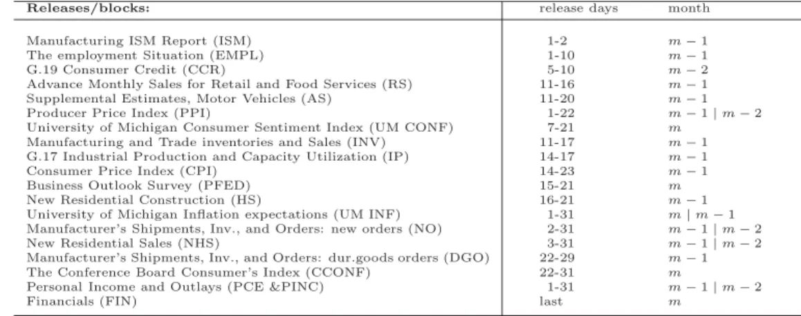
are released through regular scheduled macroeconomic reports which are released on different dates and with varying degree of delays. Variables belonging to the same report are released together hence they are grouped by blocks. Tables A.1 and A.2 in the Appendix provide a description of the variables belonging to each report as well as the transformation applied to the variables. The timing of the block releases is shown in Table A.3 where
the second column gives the typical range, in days, in monthm in which a
given block is released, and the third column refers to the month to which it pertains. Note also that the order of block releases is non constant as illustrated by the fact that the ranges overlap.
8Last is simply the last day of the month.
9
For most variables, the first release is a preliminary figure, containing noise and/or based on incomplete information, and is subject to subsequent revisions.
10
The nowcasts computed using vintages available in the quarter following the reference quarter are backcasts, however since these vintages, up to the end of the second month, are still unbalanced for the current quarter, we also name them nowcasts.
11
Note that within the nominal group there are some financial variables, the fed fund rates and term and credit spreads, which are observed at the daily frequency. To convert them to monthly frequency, we aggregate daily price changes over the month, and update these variables only on the last day of every month. This corresponds to GRS treatment of financial variables.
These real-time vintages, in conjunction with GRS approximation to the P roj(GDPq0 |Ωd,m) denoted as GDPq0|vd,m, which is explained in the next
section, enable us to construct, and as a by-product update, GDP nowcasts
as information pertaining to the reference quarter,q0, is released.
3
The model
In this section we briefly describe GRS model used to compute the nowcasts (and forecasts) of GDP according to the daily real-time data flow. For a comprehensive description of the model and the estimation technique see Giannone et al. (2008). The first part of the model consists of a parametric version of the dynamic factor model, which can be cast in the state space form and enables one to extract factors on the basis of unbalanced panels and to forecast factors. The second part consists of a bridge equation, which allows bridging of monthly information, i.e. the factors, with quarterly GDP.
3.1 The Dynamic Factor Model
Then×1 vector of stationary standardized monthly variables,xtis assumed
to follow a dynamic factor structure. In such a model, each variablexit is
represented as the sum of two orthogonal unobserved components: a com-mon component and an idiosyncratic component. The comcom-mon component
is driven by a small number r << n of unobserved common factors that
account for most of the comovement among the variables. The idiosyncratic component is driven by variable-specific shocks.
The model can be written as:
xt=χt+ξt= Λft+ξt (1)
where χt is a n×1 vector of common components, ft is a r×1 vector of
common factors, Λ is the n×r matrix of the factor loadings, and ξt is a
n×1 vector of idiosyncratic components.
Equation (1) links the unobserved factors to the observed variables, with the additional assumption that the idiosyncratic components are cross-sectionally orthogonal white noises:
E(ξtξt) = Ψ =diag(ψ1, ..., ψn) (2)
The factors’ dynamics are specified as a vector autoregression (VAR) of order p:
ft=A1ft−1+...+Apft−p+But; utW N(0, Iq) (4)
whereA1, ..., Ap arer×rmatrices of autoregressive coefficients, B is ar×q
matrix of rank q, ut is the q dimensional white noise process of common
shocks and it is further assumed that the stochastic process for ft is
sta-tionary. It is also assumed that these shocks, ut, are orthogonal to the
idiosyncratic components,ξt:
E(ξtut−s) = 0, for all s (5)
Lastly, to deal with the missing observations at the end of the sample, i.e the “jagged ”edge structure of the panel, it is assumed that:
ψit=
ψi if xit is available
∞ if xit is not available (6)
The estimation method is the two-step estimator of Doz et al. (2006a). In a first step the factors in Eq.(1) are extracted using principal compo-nents from a balanced panel, i.e truncating the panel at the last month for which all variables are available. This also provides estimates of the factors loadings and the covariance matrix of the idiosyncratic components. Next the parameters of Eq.(4) are estimated by running a VAR on the estimated factors. In a second step the model described by Eqs.(1)-(6) is cast in the state space form, and replacing the parameters by their consistent estimates obtained from the first step, the factors are re-estimated recursively using the Kalman filter and smoother. Given the assumption on the variance of the idiosyncratic component, the Kalman filter will put a zero weight on missing observations when updating the factors. In practice we implement this by using a selection matrix applied to the measurement equation (see
Koopman and Durbin (2001),§4.8).
This estimator is consistent for large sample size, T, and cross-section
dimension, n, and robust to serial and cross-sectional correlation of the
idiosyncratic component. Furthermore, Doz et al. (2006b) show that by iterating on the two-step estimator one obtains quasi-maximum likelihood estimates.
3.2 The bridge equation
The first part of the model, as described above, allows one to extract monthly factors which summarize the information available up to that day in the un-balanced panel. The second part consists in bridging these monthly factors with quarterly GDP growth to obtain a nowcast (forecast) of current quar-ter (h quarquar-ter ahead) GDP growth as measured by the quarquar-ter over quarquar-ter growth rate of real GDP.
Notice that prior to estimation of the factors, the stationary monthly variables are aggregated such that they, and the factors estimates, represent a quarterly quantity in the last month of the quarter. Hence, in the third
month of a reference quarter one directly obtains ˆF3q0|3q0, and in the first
two months one obtains a forecast of the factors for the third and second
months, ˆF3q0|3q0−2 and ˆF3q0|3q0−1 respectively, using Eq.(4). To compute the
nowcasts from the following quarter vintages, i.e. the backcasts, one uses ˆ
F3q0|3q1−k wherek= 2,1,0.
The GDP nowcast on any day is then obtained as a projection of GDP on these quarterly factors:
GDPq0|Ωd,m = ˆα+ ˆβFˆ3q0|d,m
where d= 1, ..., last, m = 3q0−k,3q1−k and k= 2,1,0. The coefficients
of the projection are estimated by OLS regression of GDP on the quarterly factors from the sample of available data for GDP. Similarly, iterating for-ward the forecasts of the factors using Eq.(4), one obtains h quarters ahead forecasts of GDP, as follows:
GDPqh|Ωd,m = ˆα+ ˆβFˆ3qh|d,m.
4
The empirical results
4.1 Model specifications, GDP data and benchmarks Model specifications
To specify the model one has to set the number of static and dynamic
factors and the number of lags of Eq.(4),r,q andp respectively.We present
results for five different specifications over the ranger= 1, ...,15, q=r, ...,8
specification for most days for each horizon, i.e. which produces the smallest
mean square forecast error.12 Secondly, we consider forecast averages over
all combinations of r, q and p. The third and fourth specifications are
the ones that maximize ex-ante the in-sample fit, i.e. the bridge equation estimated from the sample of available GDP data. The models are selected using the Akaike and Bayesian information criteria respectively. Lastly, we
use Bai and Ng (2002) and Bai and Ng (2007) information criteria to selectr
andq respectively and the Bayesian information criterion to selectp. These
last three specifications are updated at the beginning of each quarter.13
These five specifications are thereafter denoted by best, aver., AIC, SBC and B&N respectively. The model parameters and factors are estimated recursively using only information available at that time and re-estimated at every information release.
GDP data
An issue arises regarding the choice of which GDP data should be used as actual for nowcasts (forecasts) evaluation. The latest vintage is the one closer to true GDP growth, but it includes the benchmark revisions, which a real-time forecaster cannot anticipate. As aforementioned, three successive real-time (initial) estimates of GDP for a reference quarter are released during the following quarter. The first estimate is based on incomplete information, and is subsequently revised as more data becomes available as well as with revisions to previously released figures. These second and third estimates are then based on source data for the three months of the quarter they cover. We report results using the second, i.e. preliminary, estimate of GDP as target variable as this more closely measures what a forecaster predicts and what a decision maker will use in real-time, as it is less noisy
than the first estimate.14
Benchmarks
We compare the GRS model performance against two standard univari-ate benchmarks used in the forecasting literature. Firstly, an autoregressive
12In general no specification is uniformly best for all days of the quarter.
13
Since a balanced panel is needed to compute the Bai and Ng information criteria, the specification does not change on a daily basis with information releases. Although, the daily updating of vintages also include revisions to past values, it does not change the specification chosen.
14
The results using the third estimate are very similar to those using the second estimate as the correlation between those two series is 0.9. We also report results in the Appendix using GDP revised, as of November 23, 2010, as target.
(AR) model whose lag length p is selected recursively using the Bayesian
information criteria with a maximum of p = 6. Secondly a naive constant
growth model (RW) of no predictability (random walk in levels), which sim-ply predicts GDP growth to be equal to the average of past growth. These models are estimated using real-time data and updated with each GDP re-lease, i.e. including the successive GDP revisions. We also compare the model performance to the SPF which is a quarterly survey that presents consensus forecasts from private professional forecasters and is a known benchmark difficult to beat. This survey is conducted by the PFED around the middle of the quarter.
4.2 The daily evolution of the nowcasts
The model nowcasting performance is evaluated over the sample period
q4-2000 (q0 = 1) to q1-2010 (q0 =Q) using the mean square forecast errors15
(MSFE) statistic which is defined as follows: M SF Eq0
d,m = Q1
Q
q0=1(GDPq0|d,m−GDPq0)2,
whered= 1, ..., last16 and m= 3q0−2,3q0−1,3q0,3q1−2,3q1−1,3q1.
Figure 2 below shows the daily evolution of the MSFE of GDP
now-casts17 along the real-time data flow during the current (q0) and subsequent
quarter (q1). Moreover as releases during a given quarter pertain to previous
and current quarter developments, we further disentangle the incremental nowcasting power of current quarter information on the current quarter nowcasts. Hence we display the MSFEs for the nowcasts conditioning on information relating to the past quarter only and conditioning on all, i.e. current and past quarter, information releases. The vintages used to com-pute nowcasts with previous quarter information only are constructed from the real-time vintages, and thus include the latest releases and revisions per-taining to the previous quarter released in the current quarter, but where any available information for the reference quarter is disregarded, i.e. it is treated as missing.
15Note that MSFE are presented on an non annualized basis.
16
Last is simply the last day of the month, i.e. d = 28,29,30 or 31. In this way,
all months have the same number of nowcasts, and hence MSFE for a given dayd are
computed on the basis of the same number of observations over the sample period.
17
Each time there is a release, i.e. the latest value of an indicator and/or revision to previously released figures, the nowcast is updated by the news component of this release.
F ig u re 2 : D a il y ev o lut io n (duri n g the cu rre n t & n ex t q ua rt er ) o f M SF E o f G D P no w ca st s 01 10 20 01 10 20 01 10 20 01 10 20 01 10 20 01 10 20 0 0.05 0.1 0.15 0.2 0.25 0.3 0.35 0.4
info previous quarter info on previous & current quarter SPF
01 10 20 01 10 20 01 10 20 01 10 20 01 10 20 01 10 20 0 0.05 0.1 0.15 0.2 0.25 0.3 0.35 0.4 01 10 20 01 10 20 01 10 20 01 10 20 01 10 20 01 10 20 0 0.05 0.1 0.15 0.2 0.25 0.3 0.35 0.4 01 10 20 01 10 20 01 10 20 01 10 20 01 10 20 01 10 20 0 0.05 0.1 0.15 0.2 0.25 0.3 0.35 0.4 01 10 20 01 10 20 01 10 20 01 10 20 01 10 20 01 10 20 0 0.05 0.1 0.15 0.2 0.25 0.3 0.35 0.4
Best (ex−post) AIC (in−sample)
Average m1−q0 m1−q0 m1−q0 m2−q0 m2−q0 m2−q0 m1−q0 m2−q0 m2−q0 m1−q0 m3−q0 m3−q0 m1−q1 m1−q1 m1−q1 m3−q0 m1−q1 m3−q0 m2−q1 m2−q1 m3−q1 m2−q1 m3−q1 m3−q1 m3−q1 m2−q1 m1−q1 m3−q1 SBC (in−sample) B&N m3−q0
balanced panel for the previous quarter balanced panel for the current quarter
Given publication lags, up to the middle of the 1st month, the releases are all pertaining to the previous quarter and hence the MSFEs, using both information sets, coincide. The first current quarter information comes with the release of soft data (the business outlook survey of the PFED and the consumer confidence index of the University of Michigan) and produce a noticeable decrease in MSFE of the nowcasts which includes all available information. Then, as we move forward, more information, especially hard data, on the current quarter is released, and the precision of these nowcasts increases (although not monotonically) for all specifications as well as their performance relative to the ones which use only previous quarter informa-tion. This highlights the importance of incorporating the available current quarter information on the accuracy of the estimate as well as for competing with professional forecasters (SPF) who exploit timely information. Notice that in Figure 2 we did not display the MSFE of the univariate benchmarks, i.e. the AR and RW models, as they are nearly twice that of the model and the SPF, but are shown in Table 2 of the next section.
Note also that at the end of the second month of the current quarter one has a balanced panel for the previous quarter and the MSFEs conditioning on previous quarter information only show the performance of a traditional, i.e. balanced panel, factor model. Not surprisingly it is much worse than that of the model which takes into account the “ragged”edge structure of the panel. Moreover, the further updating of these nowcasts only relates to revisions of previously released figures, and do not increase much the precision of the signal anymore. The same applies to the nowcasts conditioning on all information throughout the end of the second month of the following quarter. Notice also that the strong decrease in MSFE at the beginning of the second month of the next quarter is due to the release of GDP advance estimate for the reference quarter. From that point onwards the model does not perform better than the advance estimate in nowcasting the preliminary or final figures.
Table 1 below further summarizes the impact of all information releases on the accuracy of the nowcast up to the release of the target GDP. It displays the ratio of the MSFEs of nowcasts at different dates relative to the one on the first day of the quarter. For all specifications, the MSFEs have decreased by more than 50% by the end of the reference quarter and by 65% to 80% the day before the target is released.
Table 1: Relative MSFEs (versus first day ofq0)
specification Best Aver. AIC BIC B&N nowcasts date end 1st monthq0 0.68 0.71 0.65 0.75 0.67 end 2nd monthq0 0.48 0.56 0.48 0.56 0.52 end 3rd monthq0 0.39 0.42 0.37 0.45 0.48 end 1st monthq1 0.23 0.29 0.29 0.36 0.29 end 2nd monthq1 0.19 0.24 0.25 0.33 0.25
Does the SPF add to GRS model nowcasts?
GRS model and the SPF are both pretty good at nowcasting (compared to univariate models), as they exploit a lot of timely information. This is further illustrated in Figure 3 below which displays the different nowcasts along with actual GDP growth. It shows that the data-rich methods track well GDP growth and nowcasted the strong decrease during the 2007-2009 recession in q4-08 and q1-09 and the upsurge thereafter. Note that the GRS model nowcasts in Figure 3, as well as subsequently, are obviously computed using all the information releases available in real-time.
The SPF, in addition to incorporating judgment, is presumably relying on more information than the model which is constrained by the real-time vintages, but it is compiled just before the middle of the quarter. The model on the other hand is an automatic, judgment free, procedure that can be updated at any time, hence can incorporate the impact of the latest infor-mation releases on its nowcasts. This additional inforinfor-mation substantially increases the precision of the model nowcasts as shown previously (see Fig-ure 2 and Table 1) in absolute and relative (to the SPF) terms. Yet the fact that the model nowcasts produce smaller MSFEs does not necessarily imply that it carries all the information available in the SPF nowcast. In the sequel we will thus assess whether these nowcasts contain incremental infor-mation for GDP upon each other, using Fair and Shiller (1990) procedure and estimate the following regression:
GDPq0 =α0+βz0GDP
z
q0|Ωd,m+β
SP F
0 GDPSP Fq0 +ε0 (7)
wherez=F Mbest,F Maver.,F MAIC,F MSBC, andF MB&N. This procedure
was also used by Romer and Romer (2000) to test whether the Fed Green-book (GB) forecasts were superior to private sector forecasts. The SPF does not contain additional information with respect to the model nowcasts if and
only ifβ0SP F is not significantly different from zero andβ0GRS is significantly
Figure 3 : Nowcasting GDP growth q4_00 q4_01 q4_02 q4_03 q4_04 q4_05 q4_06 q4_07 q4_08 q4_09q1_10 −5 0 5 GDP AR RW SPF B&Ng AIC SBC Average Best q4_00 q4_01 q4_02 q4_03 q4_04 q4_05 q4_06 q4_07 q4_08 q4_09q1_10 −5 0 5 q4_00 q4_01 q4_02 q4_03 q4_04 q4_05 q4_06 q4_07 q4_08 q4_09q1_10 −5 0 5
Nowcasts using info up to SPF deadline date
Nowcasts using info up to the end of the current quarter
Nowcasts using info up to the end of the day bf GDP preliminary release
GRS model). They both contain valuable different information if both
co-efficients are significantly different from zero.18
Table 2 shows the estimation results of Eq.(7) on different dates. The SPF is conducted and released in the second month of the reference quarter. Up to 2005, the release date of the survey ranged from day 20 to 24, since then it ranged from day 12 to 15. However, the deadline date for reporting the results ranged from day 11 to 16 up to 2005, then day 7 to 12 afterwards. To produce a realistic comparison with the SPF, we compute nowcasts using
18This procedure, although related to encompassing test, is different since it does not
impose the constrain that the parameters should sum to one. West (2001) further refers to this procedure as encompassing tests when no model is encompassing.
the vintages available in real-time on every deadline day of the SPF. We also report nowcasts computed given information available the day before SPF release and at the beginning and end of the third month of the reference quarter. For the following quarter, we report nowcasts which are conditioned on the real-time vintage available the day before GDP first estimate, since after that date neither the model nor the SPF does better than the advance estimate in nowcasting the subsequent revisions to GDP first estimate. Stars indicate whether a given coefficient is significantly different from zero at
conventional levels. The % in brackets in theR2 column is a measure of the
marginal information content of the SPF, i.e. it represents the increase in
theR2 from inclusion of the SPF compared to a regression with only GRS
model nowcasts.
Firstly note that as a preliminary step we investigated whether these nowcasts have individual predictive content for GDP by running univariate regressions. For all dates and all specifications the model nowcasts, as well as the SPF ones, are statistically significant. Secondly, during the second month of the reference quarter, the model nowcasts are highly correlated
with those of the SPF, creating problems of multicollinearity. Hence in
some instances, neither nowcasts are significant in the multivariate
regres-sion whereas they are in an univariate one.19
With respect to thebestmodel specification, the SPF does not add any
information as it is never significant, suggesting that the often cited superi-ority of the SPF, attributable to judgment, is weak over our sample. For the other specifications, the SPF is only significant around its release/deadline
date. Furthermore for all specifications, the R2 increases as more
informa-tion on the current quarter is released, whereas the contribuinforma-tion from the SPF decreases and its marginal information content is zero from the third month of the reference quarter onwards. The point estimates of the coeffi-cients further suggest that an optimal nowcast would put a weight close to zero on the SPF and close to one for the model by the third month.
These results show that the model performs well compared to the SPF, which is a known benchmark difficult to beat. Furthermore, as one moves forward along the real-time data flow the model nowcasts can be updated,
19
When re-estimating Eq.(7) and using the part of the SPF which is orthogonal to the model nowcast one finds that the model is indeed significant. This part is simply the residual of a regression of the SPF on the model nowcast, which by construction of the ordinary least squares estimator is orthogonal to the model nowcast. The same holds true for the SPF if one uses the part of the model nowcast which is orthogonal to the SPF.
Table 2: Marginal information content of the nowcasts
Best
forecasts dates: αh βF M,Best
h βSP Fh R2h
SPF deadline day -0.28 0.56 0.63 63% (7%)
day bf SPF release -0.26 0.67 0.51 65% (4%)
beg. of 3rd month -0.17 0.95 0.23 69% (1%)
end of 3rd month 0.15 0.99 0.07 72% (0%)
day bf GDP adv. release 0.44 1.14 -0.16 79% (0%)
Average
forecasts dates: αh βF M,Av.
h βSP Fh R2h
SPF deadline day 0.18 -0.08 1.09 59% (14%)
day bf SPF release 0.09 0.11 0.94 59% (8%)
beg. of 3rd month 0.05 0.60 0.49 61% (1%)
end of 3rd month 0.18 1.27 -0.18 68% (0%)
day bf GDP adv. release 0.49 1.14 -0.14 71% (0%)
AIC
forecasts dates: αh βF M,AIC
h βSP Fh R2h
SPF deadline day 0.14 -0.02 1.04 59% (15%)
day bf SPF release 0.07 0.30 0.77 60% (7%)
beg. of 3rd month 0.17 0.63 0.41 64% (2%)
end of 3rd month 0.46 1.00 -0.03 70% (0%)
day bf GDP adv. release 0.55 0.78 0.16 70% (0%)
BIC forecasts dates: αh βhF M,SBC βSP Fh R2h SPF deadline day 0.19 -0.16 1.15 59% (16%) day bf SPF release 0.14 -0.04 1.06 59% (11%) beg. of 3rd month 0.15 0.45 0.59 61% (2%) end of 3rd month 0.34 0.86 0.15 66% (0%)
day bf GDP adv. release 0.65 0.88 0.06 69% (0%)
B&N
forecasts dates: αh βF M,B&N
h βSP Fh R2h
SPF deadline day -0.03 0.35 0.75 61% (8%)
day bf SPF release -0.04 0.56 0.54 63% (4%)
beg. of 3rd month 0.16 0.80 0.26 66% (1%)
end of 3rd month 0.47 0.81 0.14 68% (0%)
day bf GDP adv. release 0.60 0.75 0.16 71% (0%)
Notes: The stars next to the estimated coefficients reports the significance level:sign. at 10%,sign. at 5%,sign. at 1%. The stars in brackets refer to the univariate significance level of the forecasts, i.e. significance ofβzhinGDPqh=αzh+βzhGDPz
qh+εh,
wherez=SP F,Best,B&N,Aver.andhis the forecast horizon. The % in brackets in the
R2hcolumns are the marginal (relative to a regression with only FM forecasts) predictive power of the SPF. All standard errors are corrected for heteroskedasticity and serial correlation overh−1quarters. The target is GDP 2nd estimate.
hence incorporate the impact of the latest information releases, whereas the SPF becomes stale. This continuous updating of the model nowcasts increases the precision of the estimate, thus is more valuable to policy-makers, financial market participants and businesses who need the most up to date assessment of the state of the economy.
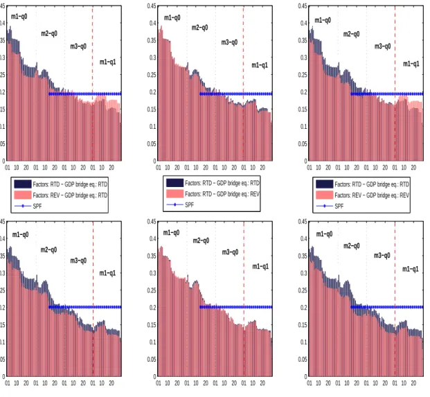
Real-time versus revised data
In this section we briefly evaluate the sensitivity of the results to real-time versus revised data, and constructed pseudo real-real-time vintages for the period October 1, 2000 to June 30, 2010. For each day over that period, we
construct a vintage reproducing the pattern of real-time missing observations
but using the latest released values for each series as of June 30, 2010.20
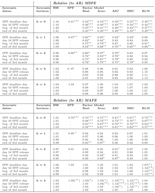
The percentage of total panel variance explained by the first few static and dynamic principal components is quite similar for the real-time and re-vised panels, indicating that the degree of comovement between the variables is robust to the revisions issue. In the nowcasting exercise we show results for different specifications which are however not the same when using real-time and revised data which makes the comparison difficult. For example, the best specification using real-time data is not necessarily among the one giving the smallest MSFE when evaluated with revised data, and vice versa. We thus present the result only for the nowcasts computed by averaging over all specifications. Furthermore, the real-time versus revised data issue also applies to GDP data since they are used to construct the nowcast in the bridge equation and are the target against which the nowcast are measured. Hence to fully assess the impact of data revisions one has to consider four cases for a given GDP target , i.e. real-time and revised. For each target we compute nowcasts using real-time and revised vintages for the panel of monthly variables and real-time and revised GDP for the bridge equation. Then each of the four cases are evaluated against real-time and revised GDP as target. The results are shown in Figure A.1 of the Appendix.
First let us consider the graphs in the second row of Figure A.1. When nowcasting revised GDP, one obtains, on average, smaller MSFE if one uses revised data instead of real-time data. However the upper row of the figure shows that when the target is real-time GDP the results are more mixed. At the beginning of the quarter, revised data produce smaller MSFE, but from the beginning of the third month onwards, i.e. when one has some hard data for the current quarter, real-time data produce better estimates, on average. Note that when considering all the different specifications individually one cannot establish a clear ranking for a given target between real-time and revised data throughout the quarter and over horizons.
20
For example, for industrial production the real-time vintage as of March 25, 2002 includes the latest values of the series up to February 2002, released on the March 15, 2002. The pseudo real-time vintage as of March 25, 2002 will also include the values of industrial production up to February 2002, but using its latest released values in our sample on June 30, 2010.
4.3 Real-time now-and-forecasting competition
In this section we further ran a forecast horse race between the timely and data-rich forecasts, i.e. GRS model and the SPF, and the two univariate models, i.e. the AR and RW.
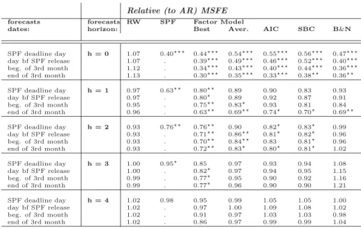
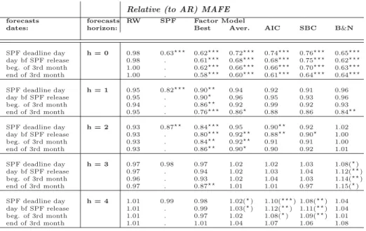
Table 3 below reports the predictive ability of all the different forecasts relative to those of the AR benchmark, i.e. relative MSFEs (RMSFEs). As a robustness check we display similar results in Table A.4 of the Appendix using relative mean absolute forecast errors (RMAFE) as a performance criteria. A number below one indicates forecasts that are more precise, on average, than the benchmark, and stars imply that the difference is
statis-tically significant.21
• For horizon h= 0, the SPF and all specifications of GRS model
out-perform by far the AR benchmark, with improvements in nowcasting accuracy of the order of 45% to 70%. Furthermore, these sizable gains are highly significant, as illustrated by the concentration of stars in the upper left part of table.
• Turning to the pure forecasts, the SPF and thebest specification
out-perform the AR, but significantly so only for forecasts horizons up to
h= 3. For the other factor model specifications, there are also some
significant gains up to horizonh = 2. Lastly, the improvement in
fore-cast accuracy from the data-rich methods decrease with the forefore-cast horizon as the RMSFE increases as one moves downwards in the table.
• The RW performs quite similarly to the AR model at forecasting as
the RMSFEs are close to one and slightly worse at nowcasting.
These results show that GRS model and the SPF outperform the AR for
short-term forecasting. The gains in forecasting accuracy for horizonsh >0
are however of smaller order of magnitude compared to those of the nowcasts, suggesting that exploiting the latest available information on the current quarter does not help as much for forecasting as it does for nowcasting. As the forecast horizon increases, RMSFEs tend to be close to one for all models,
implying similar performance. Qualitatively similar results are obtained
21The Diebold-Mariano (1995) and West (1996) procedure is used to test for equal
predictive ability of two models. This procedure applies to non-nested models under the null and hence we do not perform any tests using the RW since this would imply nested
Table 3: Relative (to AR) MSFE
Relative (to AR) MSFE
forecasts forecasts RW SPF Factor Model
dates: horizon: Best Aver. AIC SBC B&N
SPF deadline day h = 0 1.07 0.40 0.44 0.54 0.55 0.56 0.47 day bf SPF release 1.07 . 0.39 0.49 0.46 0.52 0.40 beg. of 3rd month 1.12 . 0.34 0.43 0.40 0.44 0.36 end of 3rd month 1.13 . 0.30 0.35 0.33 0.38 0.36 SPF deadline day h = 1 0.97 0.63 0.80 0.89 0.90 0.83 0.93 day bf SPF release 0.97 . 0.80 0.89 0.92 0.87 0.91 beg. of 3rd month 0.95 . 0.75 0.83 0.93 0.81 0.84 end of 3rd month 0.96 . 0.63 0.69 0.74 0.70 0.69 SPF deadline day h = 2 0.93 0.76 0.76 0.90 0.82 0.83 0.99 day bf SPF release 0.93 . 0.71 0.86 0.81 0.82 0.96 beg. of 3rd month 0.93 . 0.70 0.84 0.83 0.81 0.96 end of 3rd month 0.93 . 0.72 0.83 0.80 0.81 1.02 SPF deadline day h = 3 1.00 0.95 0.85 0.97 0.93 0.94 1.08 day bf SPF release 1.00 . 0.82 0.97 0.94 0.95 1.15 beg. of 3rd month 0.99 . 0.77 0.95 0.90 0.92 1.16 end of 3rd month 0.99 . 0.77 0.96 0.90 0.90 1.21 SPF deadline day h = 4 1.02 0.98 0.95 0.99 1.05 1.05 1.00 day bf SPF release 1.02 . 0.97 1.00 1.09 1.08 1.02 beg. of 3rd month 1.02 . 0.91 0.97 1.03 1.03 0.98 end of 3rd month 1.02 . 0.86 0.97 0.99 0.99 1.04
Notes: Given the recursive scheme to generate the forecasts, the Diebold-Mariano(1995) and West(1996) procedure is used to test for equal predictive ability. Following West(2006), inference is based on the regressions: (GDPqh−GDPzqh)2−(GDPqh−GDPbenchqh )2=αh+εh and
|GDPqh−GDPzqh|−|GDPqh−GDPbenchqh |=αh+εh for MSFE, where h is the forecast horizon, and
z=SP F,F MBest,F MB&N ,F MAver. ,RW and bench=AR in the upper part of the table and
z=F MBest,F MB&N ,F MAver. andbench=SP F in the lower part of the table. The estimate ofαis
the difference in performance between model-zand the benchmark. The null of equal predictive ability
isH0:αh=0vsH1:αh<0(in brackets results of the same null vsH1:αh>0. Under the null, the limiting
behavior of the test is standard. Standard errors are corrected for heteroskedasticity and serial correla-tion over h-1 quarters. Stars denote rejeccorrela-tion of the null at 1%(), 5%() and 10%() significance levels. The target is GDP 2nd estimate.
using RMAFEs and/or GDP revised as target and are reported in Tables A.4 and A.5 of the Appendix.
Faust and Wright (2007) using a different methodology over an earlier sample and with a different objective find similar results. They aimed at evaluating whether the well documented superiority of the Federal Reserve (Fed) in forecasting is due to an inherent advantage or to their better esti-mate of the current state of the economy. They do not take into account the real-time data flow and hence use models which rely on a balanced panel. They use real-time vintages synchronized with the GB and append the GB forecasts to the actual data, providing the models with a balanced panel up to previous or current quarter. They find that the GB superiority is confined to nowcasting, as when the models have information up to the previous, the Fed forecasts dominate only at horizon h=0, and when the models have
information up to the current quarter the GBs advantage disappears.22 These findings concerning pure forecasting are consistent with those of d’Agostino et al. (2006) who found that since the Great Moderation, the predictability of GDP is mainly found at short horizons. The fact that the AR model which relies solely on the dynamics of GDP performs rather similarly to the RW is further evidence that this near-term predictable com-ponent can only be extracted from the timely information available in the numerous monthly conjunctural indicators as in the SPF and GRS model. Furthermore, contrary to nowcasting, there simply is not much scope for an advantage in forecasting far ahead whether it be from institutional forecast-ers or from an automatic procedure that exploit rich and timely information.
4.4 What about the current recession?
The results up to now were for the full-sample period which includes the 2007-2009 recession. However, it is well known that forecasting recessions and business cycle turning points is difficult. Stock and Watson (2003), henceforth SW, looking at the 2001 recession, found that the SPF per-formed quite poorly and that although a few leading indicators predicted a slowdown, they strongly under-estimated it. They also noted that individ-ual predictive relationships are unstable, as the indicators leading the 2001 recession were different from those leading the 1990 recession. McCracken (2009), further documents that the SPF have tended to be less precise during recessions.
In this section we hence also analyze the predictive ability of all the different forecasts for and during the current recession. According to the NBER dating procedure the recession started in q4-07 and ended in q2-09. Table 4 below displays the (annualized) quarter-on-quarter growth of real GDP over the recession, as measured in real-time, i.e. the 1st, 2nd and 3rd
estimates, as well as in subsequently revised vintages of November 2010.23
As estimated in real-time, over the first three quarters of the recession, GDP growth was still positive and non negligible in q2-08. According to the re-vised figures, the first recession quarter q4-07 was strongly rere-vised upwards whereas most of the subsequent quarters were revised downwards, with the sharpest revision occurring for q3-08. Hence, from today’s perspective, i.e.
22However, for inflation the GB forecasts are still superior.
23
Note that the revised vintage includes also the benchmark revision which occurred in July 2009.
with revised data, the 2007-2009 recession appears deeper than first esti-mated in real-time.
Table 4: Actual quarter-on-quarter real GDP growth
q4-07 q1-08 q2-08 q3-08 q4-08 q1-09 q2-09 1st est. 0.6 0.6 1.9 -0.3 -3.9 -6.3 -1.0
2nd est. 0.6 0.9 3.2 -0.5 -6.4 -5.8 -1.0
3rd est. 0.6 1.0 2.8 -0.5 -6.5 -5.6 -0.7
revised 2.9 -0.7 0.6 -4.1 -7.0 -5.0 -0.7
Table A.7 in the Appendix, which draws on SW (2003), displays the forecasts for and over the current recession. The first column reports the quarter being forecasted along with the GDP outturns as measured from a real-time and revised perspective and the second column displays the name of the model used to generate the forecasts for each reference quarter. The subsequent columns correspond to the quarters in which the forecasts are
made for a given row. For the pure forecasts we show theh−step ahead
forecasts computed from the univariate and factor models conditioning on information available on the SPF deadline date and at the beginning and
end of the third month of q0. For the nowcasts, we further provide the
backcast computed given the vintage available the day before GDP advance estimate is released in the following quarter. Hence fixing a line and going from left to right, tells us how the forecasts for a given quarter evolve as
the time to that quarter decreases.24 Fixing a column and going downwards
gives the forecasts (h= 0 toh= 4) for future dates from the perspective of
information available in a given quarter.
During the course of 2007, neither univariate nor data-rich methods had factored in the possibility of a recession. Only once when growth was near zero as estimated in real-time, did data-rich forecasts start to predict slower
growth (but still positive) over the next quarter or two. As we moved
through the recession, data-rich forecasts were decreasing.25 But neither
predicted anything close to the sharp deterioration in q4-08 and q1-09. It’s only once q4-08 (-6.4%) unfolded, that forecasts became negative. Turning to the nowcasts the SPF and the model did well and nowcasted the strong decrease in q4-08 and q1-09. The only exception is q2-08, for which both predicted near zero growth whereas the preliminary estimate was 3.2% but then revised to 0.6%. The univariate models for their part did very badly during the downturn. As they relied solely on past GDP realizations, they
24
It simply displays forecasts for horizonsh= 4 toh= 0.
were very slow to adapt. For example, the AR nowcasts turned negative only in q1-09, once it was based on the strong negative outturn of q4-08, and then in q2-09, it strongly underestimated growth as it followed the two consecutives worse quarters in the recession.
From the evidence presented above none of the forecasting method an-ticipated the recession, nevertheless the data-rich forecasts adapted more quickly and still produced good nowcasts. This is further illustrated in Ta-ble A.6 of the Appendix which displays the relative RMSFE of the different forecasts against the AR benchmark for the full-sample period, i.e. up to q1-10, relative to those excluding the recent crisis, i.e. up to q3-07. Note that these ratios are also the RMSFE of a given forecast up to q1-10 rela-tive to those up to q3-07 divided by the same relarela-tive RMSFE for the AR benchmark. Although, for all models absolute forecasting performance
de-teriorates when including the recession period26, the relative performance of
the data-rich methods, whether survey or model based, over the univariate methods did not. As shown in Table A.6 the ratios are mostly smaller than one, indicating that their forecasting performance deteriorated less than those of the benchmark.
5
Conclusion
This paper evaluates the nowcasting and forecasting performance of the Gi-annone et al. (2008) factor model in a fully real-time setting and also over the extended period including the current recession. To this end, we have constructed a novel database of vintages for a panel of US macroeconomic variables which enables us to reproduce the information available to a fore-caster in real-time. Analogously to GRS pseudo real-time results, we find that as more information on the current quarter is released, the precision of the nowcast increases substantially and that the model tracks well the strong worsening of growth during the recent recession. The results show that the model performs well compared to the SPF, which is a known benchmark difficult to beat. Indeed, the SPF does not carry additional information with respect to the model best specification, suggesting that the often cited superiority of the SPF, attributable to judgment, is weak over our sample. Then, as one moves forward along the real-time data flow, the continuous
26
We did not show the table but for all methods and all horizons, MSFE and MAFE are always bigger over the whole sample period compared to those over the sample ending in q3-07.
updating of the model provides a more precise estimate of current quarter GDP growth and the SPF becomes stale compared to all the model specifica-tions, thus is more valuable to policy-makers, financial market participants and businesses who need the most up to date assessment of the state of the economy.
References
[1] Aastveit, K., & Trovik, T. (2007).Nowcasting Norwegian GDP: the role
of asset prices in a small open economy. Norges Bank Working paper
2007/09.
[2] Angelini, E., Camba-M´endez, Giannone, D., R¨unstler, G., & Reichlin,
L. (2008).Short-term forecasts of euro area GDP growth.Working paper
series 953, European Central Bank.
[3] Bai, J., & Ng, S. (2002). Determining the Number of Factors in
Ap-proximate Factor Models. Econometrica,70,191-221.
[4] Bai, J., & Ng, S. (2007). Determining the Number of Primitive Shocks
in Factor Models. Journal of Business and Economic Statistics
,25,52-60.
[5] Ba´nbura, M., Giannone, D. & Reichlin, L. (2010).Nowcasting.Working
paper series 1275, European Central Bank.
[6] Ba´nbura, M., & Modugno, M. (2010). Maximum likelihood estimation
of large factor model on datsets with arbitrary pattern of missing data. Working paper series 1189, European Central Bank.
[7] Ba´nbura, M., & R¨unstler, G. (2011). A look into the factor model black
box: Publication lags and the role of hard and soft data in forecasting
GDP. International Journal of Forecasting,27,333-346.
[8] Barhoumi, K., Benk, S., Cristadoro, R., Den Reijer, A., Jakaitiene,
A., Jelonek, P., Rua, A., R¨unstler, G., Ruth, K., & Van
Nieuwen-huyze, C. (2009). Short-term forecasting of GDP using large monthly
datasets: a pseudo real-time forecast evaluation exercice. Journal of
Forecasting,28,595-611.
[9] Bernanke, B.S., & Boivin, J.(2003). Monetary policy in a data-rich
Environment. Journal of Monetary Economics,50,525-546.
[10] Boivin, J., & Ng, S. (2005). Understanding and comparing factor-based
forecasts. International Journal of Central Banking,3(1),117-151.
[11] D’Agostino, A., Giannone, D., & Surico, P. (2006). (Un)predictability
and macroeconomic stability.Working paper series 605, European
[12] D’Agostino A., & Giannone, D. (2006). Comparing alternative
predic-tors based on large-panel factor models stability,”Working paper series
680, European Central Bank.
[13] D’Agostino, A., McQuinn, K., & O’Brien, D. (2008).Now-casting Irish
GDP. Research technical paper 9/RT/08, Central Bank of Ireland.
[14] Dehon, C., Gassner, M., & Verardi, V. (2009). Practitioners’ corner.
Beware of good outliers and overoptimistic conclusions.Oxford Bulletin
of Economics and Statistics,71-3,437-452.
[15] Diebold, F.X., & Mariano, R.S. (1995). Comparing predictive accuracy.
Journal of Business and Economic Statistics,13,253-263.
[16] Doz, C., Giannone, D., & Reichlin, L. (2006a). A two-step estimator for large approximate dynamic factor models based on Kalman filtering. Journal of Econometrics, forthcoming.
[17] Doz, C., Giannone, D., & Reichlin, L.) A Two-Step a quasi maximum
likelihood approach for large approximate dynamic factor models.
Dis-cussion paper 5724, CEPR.
[18] Durbin, J., & Koopman, S.J. (2001).Time series analysis by state space
methods. Oxford University Press.
[19] Fair, R.C., & Shiller, R.J. (1990). Comparing information in
fore-casts from econometric models.The American Economic Review,Vol.80
NO.3,375-389.
[20] Faust, J., & Wright, J.H. (2009). Comparing Greenbook and reduced
form forecasts using a large realtime dataset. Journal of Business and
Economic Statistics,27:4,468-479.
[21] Forni, M., Hallin, M., Lippi, M., & Reichlin, L. (2005). The generalized
dynamic factor model: One-sided estimation and forecasting. Journal
of the American Statistical Association,100(471),830-840.
[22] Giannone, D., Reichlin, L. & Sala, L. (2004). Monetary policy in real
time. NBER Macroeconomics Annual (pp. 161-200).
[23] Giannone, D., Reichlin, L. & Small, D. (2008). Nowcasting: The
real-time informational content of macroeconomic data. Journal of
[24] Kitchen, J., & Monaco, R. (2003). Real-time forecasting in practise.
Business Economics,October,10-19.
[25] Marcellino, M., & Schumacher, C. (2008). Factor-MIDAS for now-and
forecasting with ragged-edge data: A model comparison for German
GDP. Working Paper series, ECO 2008/16, European University
In-stitute.
[26] McCracken, M.W.(2009). How accurate are forecasts in a recession?
Federal Reserve Bank of St. Louis, Economic Synopses,2009,NO.9. [27] Romer, C.D., & Romer, D.H. (2000). Federal reserve information and
the behavior of interest rates. The American Economic Review, Vol.90
NO.3,431-457.
[28] Schumacher, C. & Breitung, J. (2008). Real-time forecasting of Ger-man GDP based on a large model with monthly and quarterly data.
International Journal of Forecasting,24,386-398.
[29] Stark, T. (2010).Realistic evaluation of real-time forecasts in the survey
of professional forecasters’. Research rap - special report, Philadelphia
Federal Reserve Bank.
[30] Stock, J.H., & Watson, M.W. (2002a). Forecasting Using Principal
Components From a Large Number of Predictors.Journal of the
Amer-ican Statistical Association,97(460),147-162.
[31] Stock, J.H., & Watson, M.W. (2002b). Macroeconomic forecasting
us-ing diffusion. Journal of Business and Economic Statistics
,20(2),147-162.
[32] Stock, J.H., & Watson, M.W. (2003). How did leading indicator
fore-casts perform during the 2001 recession? Federal Reserve Bank of
Rich-mond, Economic Quarterly,Vol.89/3,Summer 2003,71-90.
[33] West, K.D. (2006). Forecast evaluation. Handbook of Economic Fore-casting, Vol. 1, Amsterdam: Elsevier.