A hybrid approach of physical laws and data-driven modeling for estimation: the example of queuing networks

(1)

modeling for estimation: the example of queuing

networks

Aude Hofleitner

Electrical Engineering and Computer Sciences

University of California at Berkeley

Technical Report No. UCB/EECS-2013-87

http://www.eecs.berkeley.edu/Pubs/TechRpts/2013/EECS-2013-87.html

(2)

Permission to make digital or hard copies of all or part of this work for

personal or classroom use is granted without fee provided that copies are

not made or distributed for profit or commercial advantage and that copies

bear this notice and the full citation on the first page. To copy otherwise, to

republish, to post on servers or to redistribute to lists, requires prior specific

permission.

(3)

by

Aude Hofleitner

A dissertation submitted in partial satisfaction of the requirements for the degree of

Doctor of Philosophy in

Electrical Engineering and Computer Science in the

Graduate Division of the

University of California, Berkeley

Committee in charge: Professor Alexandre Bayen, Chair

Professor Pieter Abbeel Professor Laurent El Ghaoui Professor Alexandre Skabardonis

(4)

(5)

Abstract

A hybrid approach of physical laws and data-driven modeling for estimation: the example of queuing networks

by

Aude Hofleitner

Doctor of Philosophy in Electrical Engineering and Computer Science University of California, Berkeley

Professor Alexandre Bayen, Chair

Mathematical models are a mathematical abstraction of the physical reality which is of great importance to understand the behavior of a system, make estimations and predictions and so on. They range from models based on physical laws to models learned empirically, as measurements are collected, and referred to as data-driven models. A model is based on a series of choices which influence its complexity and realism. These choices represent trade-offs between different competing objectives including interpretability, scalability, accuracy, adequation to the available data, robustness or computational complexity. The thesis investi-gates the advantages and disadvantages of models based on physical laws versus data-driven models through the example of signalized queuing networks such as urban transportation networks.

The dynamics of conservation flow networks are accurately represented by a first order partial differential equation. Using Hamilton-Jacobi theory, the thesis underlines the impor-tance to leverage physical laws to reconstruct missing information (e.g. signal or bottleneck characteristics) and estimate the state of the network at any time and location. Noise and uncertainty in the measurements can be integrated in the model. When measurements are sparse, the state of the network cannot be estimated at every time and location on the network. Instead, the thesis shows how to leverage other characteristics, such as periodic-ity. From deterministic dynamics, the thesis derives the probability distribution functions of physical entities (e.g. waiting time, density) by marginalizing the periodic variable. Using a Dynamic Bayesian Network formulation and exploiting the convexity structure of the sys-tem, the thesis shows how this modeling leads to realistic estimations and predictions, even when little measurements are available. Finally, the thesis investigates how sparse modeling and dimensionality reduction can provide insights on the large scale behavior of the net-work. Large scale dynamics and patterns are hard to model accurately based on physical laws. They can be discovered through data mining algorithms and integrated into physical models.

(6)

This dissertation is dedicated to my wonderful family.

To my mother, Anne. I wish I could share this achievement with you. You taught me how to embrace life and I am thankful for that everyday.

To my father, Patrick, and my sister, C´eline who have always believed in me and encouraged me.

To my boyfriend, Ryan. Your love has supported me throughout this incredible journey. I feel privileged to have you by my side everyday.

(7)

List of Figures

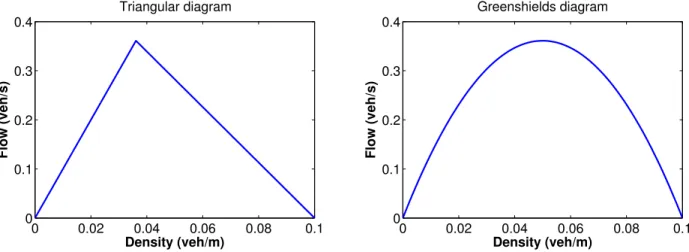
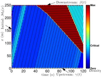
1.1 San Francisco taxi measurement locations, observed at a rate of once per minute. 10 2.1 Examples of concave flux functions (fundamental diagrams) . . . 23 3.1 Moskowitz function subject to initial and upstream value conditions . . . 29 3.2 Moskowitz function subject to initial, upstream and downstream value conditions 30 3.3 Moskowitz function subject to initial, upstream and internal value conditions . . 31 3.4 Solution of the Moskowitz Hamilton-Jacobi partial differential equation given

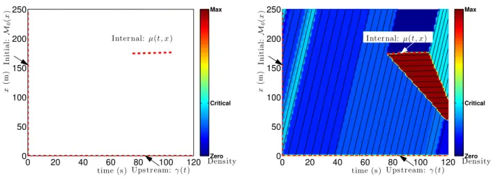
ini-tial and upstream piecewise affine boundary conditions and one affine internal value condition . . . 40 3.5 Solution of theMoskowitz Hamilton-Jacobi partial differential equation subject to

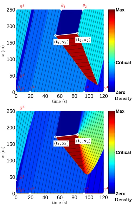
initial, upstream and downstream value conditions before solving the boundary condition reconstruction problem. . . 41 3.6 Solution of the reconstruction problem for the Moskowitz Hamilton-Jacobi partial

differential equation given initial and upstream piecewise affine value conditions and one affine internal value condition. . . 42 4.1 Deterministic solution of theMoskowitz Hamilton-Jacobi partial differential

equa-tion under given initial and upstream boundary conditions and with three differ-ent values for the capacity reduction. . . 52 4.2 Distribution of the solution of the Moskowitz Hamilton-Jacobi partial differential

equation at a fixed location, upstream of the capacity reduction. . . 53 4.3 Distribution of the solution of the Moskowitz Hamilton-Jacobi partial differential

equation at two distinct fixed times. . . 54 5.1 Space time diagram of vehicle trajectories with uniform arrivals under an

under-saturated traffic regime (top) and a congested traffic regime (bottom). . . 59 5.2 Proportion of delayed vehicles between two locations on a link . . . 61 5.3 Probability distribution of delay between arbitrary locations on an arterial linkin

the undersaturated regime. . . 62 5.4 Probability distribution of travel time between arbitrary locations on an arterial

(10)

5.5 Travel time allocation: decomposition of the path travel time into (partial) link travel times. . . 68 5.6 Routes of the network used for field test validation. The drivers drove around two

distinct loops consisting in Van Ness Ave. South bound and Franklin St. north Bound for the first routes and Van Ness Ave. North bound and Gough St. South bound for the second route. Signalized intersections are indicated with a circle. . 73 5.7 Goodness of fit of the model depending on the percentage of training data used

to learn the parameters. . . 75 5.8 Comparison of the traffic and the log-normal distributions with the empirical

distribution of travel times on two links of the network. . . 76 5.9 Performance analysis of the different travel time allocation algorithms as a

func-tion of the sampling frequency. . . 78 6.1 Schematic representation of an intersection illustrating the definition of incoming

links, outgoing links, turn ratios and vehicle assignment. . . 89 6.2 Spatio-temporal model of arterial traffic evolution represented as a Dynamic

Bayesian Network. . . 94 6.3 Schematic illustration of the resampling algorithm . . . 101 6.4 Subnetwork of San Francisco, CA used for numerical analysis of the model

per-formance. . . 105 6.5 Error metrics assessing the prediction capabilities of the Dynamic Bayesian

Net-work modeling the dynamics of traffic flow from horizontal queuing theory. . . . 109 6.6 Comparison of the model estimates with the ground truth route travel times

collected during a field test experiment in San Francisco, CA. . . 110 7.1 Two slice Temporal Bayesian Network (2TBN) representation of the model of

arterial traffic dynamics. . . 117 7.2 Distribution of vehicle location derived from horizontal queuing theory as a

func-tion of the distance from the upstream intersecfunc-tion. . . 120 7.3 Comparison of the empirical and the learned cumulative distribution of vehicle

locations. . . 127 7.4 Detection of signal locations using the spatial distribution of vehicles. . . 128 7.5 Evolution of the estimation and prediction of the percentage l₁ error on the

vali-dation dataset. . . 130 7.6 Validation of the travel time distributions computed by the model. (Left)

Evo-lution of the percentage of points in ζ_α for α _{∈ {}0.7, 0.9,0.95_}. (Right) Com-parison of the percentage of points contained in ζα with the theoretical value. . . 132

8.1 Example paths of three probe vehicles on a network. . . 148 8.2 Variation of the l₁ error in function of the regularization parameters for the l₁

and l2 penalization when encouraging sparsity on the spatial variations of traffic

(11)

8.3 Geographical representation of the traffic estimation results with detection of the spatial variation of the pace in the network. . . 151 8.4 Variation of the error metrics in function of the regularization parameters for the

l1 and l2 penalization when encouraging sparsity on the temporal variations of

traffic conditions. . . 153 8.5 Qualitative evolution of the travel time estimates on different links of the network.153 9.1 Results of the k-means algorithms on the low-dimensional projection of

network-level congestion states. The clustering exhibits different times of the day corre-sponding to different configurations of network-level congestion states. . . 161 9.2 Typical spatial configurations of traffic states for the five cluster centers of

network-level traffic states. . . 162 9.3 Examples of NMF basis, either highlighting localized correlations (top figures),

or flow-direction correlations (bottom figures). . . 164 9.4 Daily trajectories of network fluidity indices projected in 3D-NMF space exhibit

seven different typical trajectories, representing the days of the week. . . 166 A.1 Case 1: All the vehicles stop in the triangular queue. A fraction stops n_s times

in the remaining queue, the other ones stop ns−1 times. . . 194

A.2 Case 2: Some vehicles stop in the triangular queue. The others do not experience delay. . . 195 A.3 Case 3: A fraction of the vehicles stop ns times in the remaining queue. The rest

stop ns−1 times in the remaining queue. . . 196

A.4 Case 4: (Top) Case 4a: a fraction of the vehicles stop in the triangular queue and

ns times in the remaining queue, a fraction of the vehicles stop in the triangular

queue andnstimes in the remaining queue, the rest stopnstimes in the remaining

queue. (Bottom) Case 4b: a fraction of the vehicles stop in the triangular queue and ns−1 times in the remaining queue, a fraction of the vehicles stopns times

(12)

List of Tables

5.1 Outcome of statistical tests. . . 74 6.1 Error metrics representing the estimation capabilities of the Dynamic Bayesian

Network modeling the dynamics of traffic flow from horizontal queuing theory. . 107 7.1 Percentage of positive K-S tests for different values of threshold to accept the

hypothesis H0 and the two hypothesis (density model or uniform distribution). . 126

7.2 Percentage of l1 error of the model computed on a validation data set to test the

(13)

Acknowledgments

I would like to take this very special opportunity to acknowledge the importance of my family in the completion of this dissertation. My family has always supported my choices and encouraged me to seek interesting challenges and opportunities. In particular, I am grateful to my mom, Anne. She is sadly no longer among us to share this moment but I would like to emphasize her essential role in my life. She had a passion for travel, for working in international environment and socializing with people from various cultures which has strongly shaped my personality and my interests, both personally and professionally. She has always encouraged me to seek international opportunities and to benefit from the amazing cultural experiences that they provide. One of these opportunities was to go to Berkeley to join theMobile Millennium team for a one year internship, starting in July 2008. I seized the opportunity and immersed myself in an amazing project, working with incredibly interesting and welcoming people. The end of 2008 brought dramatic emotions as she unexpectedly and so suddenly passed away. I am grateful for the support I received from my dad, Patrick and my sister, C´eline as well as my family and friends following this dramatic event. When the time came to decide between starting the PhD program at UC Berkeley or coming back to France and be close to them, both my dad and sister encouraged me to continue my journey and helped me overcome this tragic life event. Despite the distance, our relationship has grown closer, stronger, and so much deeper.

I was also amazed by the attentive and personal support of my colleagues with whom I had only been working for a few months. In particular, Alex Bayen, my internship supervisor at the time, and my friend and colleague Saneesh Apte played an incredibly valuable role. The research environment at UC Berkeley had already exceeded my expectations in terms of dynamism, interest in the project and intellectual challenge; the realization that I could relate to my colleagues on the personal level as well convinced me that I wanted to pursue my graduate studies in this successful and fulfilling environment.

Since I first met him in a caf´e in Paris in the winter of 2008, Alex Bayen has struck me with his constant level of energy and excitement about the work and research of his team. The dynamism and high level of expectations appealed to me from the beginning. I was not disappointed as I arrived in Berkeley and Alex entrusted me with more responsibilities than I had ever thought I would be able to manage. Alex keeps on surprising me with his trust and the confidence that he expresses for my work and career. He always encourages me to take on new and additional challenges, pushing me beyond what I think myself capable of. The completion of this PhD can, for a fair part, be attributed to his support, contagious dynamism and will to succeed. Beyond the career drive, Alex has been of incredible personal support. Throughout the years, he has combined enjoying relaxing and social times with other fellow students from the lab, working on papers in the middle of the night, congratu-lating achievements, discussing personal matters and career choices for long hours, tirelessly editing, reshaping and improving presentation of research ideas, giving motivation and

(14)

en-ergy during low times of the PhD.

Pieter Abbeel started following my work halfway through my internship and was offering his expertise in machine learning for the arterial estimation efforts that I was pursuing. At the beginning of my PhD, Pieter pointed out an idea which I had first developed as part of a class project: simplifying the arterial traffic flow physics to model the distribution of vehicle location on a road segment. He encouraged me to develop this idea further and generalize it to travel times, in a hybrid approach of traffic theory and statistical modeling and inference. Pieter’s vision in this work turned into an essential part of my PhD work. His enthusiasm for the model, the exciting and dynamic meetings and his research directions drove my research interest far beyond my expectations.

I started collaborating with Laurent El Ghaoui through a class project which turned into a broader collaboration with one of Laurent’s students, Tarek Rabbani. Since my first intro-duction to convex optimization at Ecole Polytechnique, I have always been interested in the field. I really appreciated the opportunity that Laurent gave me to be the Graduate Student Instructor for the class Optimization models in engineering and to share my enthusiasm for the field with the students of the class.

I have had the pleasure and honor to meet and discuss research ideas with Alex Skabar-donis. I have learned a lot from his expertise in traffic and transportation. His feedback has been very important in the development and refinements of the queuing model and statistical model of urban traffic. I value the interest that he showed in a non-conventional approach to traffic modeling as well as his overall vision on the field and on its most important research questions.

I have found my best and dearest PhD collaborator in Ryan Herring. Ryan’s view to research and scientific problems seems to perfectly complement mine. Working with him has been incredibly productive and enjoyable. Between developing models, designing code architecture, taking turns at writing papers or working on class material together, we have shared a lot of the PhD joys together. Ryan was also able to help me through the times when I was less motivated about my research or was disappointed by my results. His trust in my potential to succeed and overcome obstacles has always amazed me. I feel privileged to have the chance to have someone so dear to me to celebrate the happy times of the PhD life and give me the courage and strength to overcome the deceptive times.

I benefited from the guidance and mentoring of senior PhD students who have played an important role in the completion of this dissertation. Christian Claudel introduced me to his work on viability theory. His excitement and interest for research and mathematics were contagious and lead to fruitful collaborations throughout my PhD. Saurabh Amin struck me with his mind overflowing with novel ideas and theoretical contributions. I really enjoyed our white board discussions and brainstorming sessions on traffic modeling, estimation,

(15)

statis-tics, change detection, sampling, privacy and so much more. In many ways, these discussions have inspired a lot of the research which I have pursued throughout my PhD. In particular, Saurabh had a great vision on modeling arterial traffic, focusing on defining the appropriate level of model complexity given specific estimation, sensing or control goals, which I have followed and developed in my research.

Through his work on the Path Inference Filter, Timothy Hunter has made possible a lot of the numerical validation of my work. Timothy has spent countless hours developing, implementing, improving and running his algorithm on the millions of data points received in the Mobile Millennium system everyday, to turn noisy sparse GPS measurements into filtered path travel times which can be used for traffic estimation. Anyone who has worked, looked at or even imagined working with this type of data will understand the hard and valu-able work of Timothy and realize the importance that it had in the completion of my work. Besides Timothy, the entire team of Mobile Millennium has enabled the technical support and the infrastructure to develop the numerical applications of my work. In particular, a lot of the results of this dissertation would not have been possible without the work of the team to set up and maintain the data feeds and the database, to develop the Mobile Millennium system and the road network abstraction.

The last thanks go to my friends, who I have met over the years, and have accompanied me everyday, giving advice, sharing thoughts, discussing both important and silly matters, and enjoying life. Friends have been my adopted American family and I am grateful to have met such wonderful people. I have met too many incredible people to acknowledge them individually here. I want to emphasize how much I care for their friendship, for all the moments that we have shared in the past years and the upcoming adventures which will keep on building our ties.

I still want to acknowledge a few people who have played such a wonderful role throughout my PhD. The magic of Craigslist lead me to meet Kristen Parrish and move in with her in January 2009. Even though we had barely met, Kristen warmly welcomed me and shared her personal feelings relating to losing a close family member. It was very important to have someone I could trust and confide in. Her energy and love of people was exactly what I needed at the time. I would also like to acknowledge Ana Ferreira who has been my closest friend throughout the past four years and who I hope to count as a friend in the years to come. Woody Hoburg has also been an incredible friend with whom I have been able to share a lot of personal matters, talk about awesome outdoors activities, discuss important life choices and have fun times at Mint Leaf happy hour! Finally, I am thankful for my friends in France to always be around when I come back. Keeping friendships with thousands of miles of distance is not easy and I truly appreciate these lasting friendships which are not affected by distance and time. I would not be able to go through a long PhD journey without feeling so much positive emotions, happiness and social support around me.

(16)

Chapter 1 Introduction

Queueing theory is the mathematical study of waiting lines, or queues. The field of queuing theory goes back to the early 1900s with the work of A. K. Erlang of the Copenhagen Tele-phone Company to model waiting times for calls in telecommunication networks [68, 69]. Since the 1950s, the field has received a lot of attention from the scientific community. In particular, the domains of application of queuing theory have expended from telecommuni-cation networks to general communitelecommuni-cation networks, transportation engineering, air traffic control, manufacturing or supply chain management.

Each field of application comes with its specificities in terms of the characteristics of the queuing processes, the desired features of the outcome of the mathematical analysis, the precision of the modeling and so on. For example, air traffic control has important constraints in terms of safety and models must take into account the physical characteristics of aircraft (maneuverability, minimum and maximum speed). In supply chain management, one goal is to optimize the efficiency of the entire line of production while making sure that the process is robust if a production site or engine fails. In transportation networks, the field aims at reducing the external costs due to non-optimal operations [194]. An essential step for operations and planning (routing, network optimization) is to develop the ability to estimate and forecast traffic conditions with appropriate accuracy and reliability [37].

1.1 Related work

This section reviews prior work on queuing theory. Queuing theory often refers to the analysis of a single queue. When several queues co-exist and interact, one usually refers to a queuing network. The interaction between the queues requires the development of additional modeling and statistical results on top of queuing theory results. The complexity of queuing networks often leads to (domain-specific) approximations which aim at simplifying the model and make it more tractable and computationally efficient.

(17)

Background on queuing theory

In order to analyze and optimize queuing systems, one needs a mathematical model of the physical system and its properties, known as queuing model. A queuing model is a mathematical abstraction of the reality which is typically represented by: (i) the system’s physical configuration which specifies the number and arrangement (e.g. queue capacities, queue disciplines, and so on) of the servers, which provide service to the customers, and (ii) the statistical properties of the arrival process and of the service process. The queue capacity refers to the maximum number of customers which can wait to be served in the queue. Thequeue discipline refers to the manner in which customers are selected for service when a queue has formed. There are several common queue disciplines:

• First In First Out (FIFO): the customers are served in the same order in which they have arrived. For this reason, it is sometimes also referred to asFirst Come First Serve (FCFS).

• Last In First Out (LIFO): the last customer to arrive will be the first one served, yielding another common denomination as Last Come, First Served (LCFS).

• Service In Random Order (SIRO) orRandom Selection for Service (RSS): the customer to be served is chosen randomly, independently of the arrival times.

• Priority: customers with high priority are served first.

In the context of communication networks, each communication channel is a server and the messages are the customers. The (random) times at which messages request the use of the channel characterize the arrival process, and the (random) duration to use the channel and transmit the message constitute the service process. The queue capacity may be considered infinite and the queue discipline FIFO or Priority.

Urban transportation networks are another domain of interest, used as recurring example in the remainder chapters of the dissertation. Each driver (customer) seeks to use the transportation network (server) to go from anorigin to adestination (service). In the latter queuing network, the queue capacity is defined by the number of vehicles which can fit on each road segment. The queue discipline is typically FIFO, even though some models may consider queues with priorities to model specific types of vehicles (ambulances, police vehicles and so on).

The mathematical analysis of the models aims at investigating how the physical and stochastic parameters of the system relate to certain performance measures, such as average waiting time, server utilization, throughput, probability of buffer overflow, etc. Applied queuing theory aims at developing models which are simple enough to yield to mathematical analysis, yet contain sufficient detail to reflect the behavior of the real system. This approach will remain a center component of the dissertation.

The characteristics of a queuing processes are typically defined using a notation defined by Kendall [133]. The process is described by three factors written A/S/c. Additional factors

(18)

may be used and the notation becomes A/S/c/K/D. The different factors have the following interpretation:

• A: Characteristics of the arrival process. Common denomination include Markovian (M) corresponding to Poisson arrival, Degenerate (D) corresponding to deterministic of fixed-time arrivals, Erlang (Ek) corresponding to arrivals with an Erlang

distribu-tion with shape parameter k or General (G) corresponding to arbitrary probability distribution of arrivals.

• S: Characteristics of the service process.

• c: Number of servers.

• K (optional): Capacity of the system. Once the capacity is reached, no more customers can enter the system. This factor is only mentioned when the capacity of the system is finite.

• D (optional): Queue discipline (usually not mentioned if the queue is FIFO).

Previous work has studied the properties of different queuing models including the M/D/1 and M/D/k queues [68, 69], the M/M/1 queue or the M/G/1 queue [186, 134]. The main results of queuing theory are out of the scope of this thesis. Please see [139, 48, 218, 93] for additional references on queuing theory.

Queuing networks

In many areas, such as manufacturing, transportation networks or task management (e.g. distributed computing), when a customer is serviced at a node, it can join another node and queue for service. Such a system of interacting queues is called a queuing network. The field of queuing networks is significantly more complex than the one of queuing theory with a single queue (even with several servers) because of high-dimensional interactions and dependencies.

One of the primary goals of queuing network theory is to estimate and predict the state of the network, given specific demand patterns. Statistical results aim at characterizing the robustness of the network, detecting potential bottlenecks which reduce the overall efficiency of the system or analyzing network equilibria. For a large class of networks, the policy which describes the sequence of nodes visited by a customer can be optimized. The optimization of the policy is commonly called a routing strategy.

The complexity of queuing networks benefits from specific assumptions which facilitate the analysis and understanding of the queuing processes. This thesis focuses on a class of queuing network which represent urban road networks. In numerous parts of the world, traffic congestion has a significant impact on economic activity. An essential step towards

(19)

active congestion control is the creation of accurate, reliable traffic monitoring systems. These transportation networks have the following specific characteristics.

• Signalized queuing networks: These queuing networks arise whenever two queues can-not be served concurrently and signals indicate which queue is active at a given time to manage the conflicting services. The urban (arterial) transportation network is one of the most intuitive example of signalized queuing network. Other examples include logistics and communication networks with interfering channels which cannot be used concurrently.

• Horizontal queuing networks: Queuing networks for which the amount of space of each customer is not negligible and travel speed in a queue is finite. This models the fact that once a customer is served, there is a non-null time before the next customer can be served, because it needs to “travel” to the head of the queue.

• Networks with limited and/or uncertain information: Queuing networks for which there is little and uncertain amount of information and measurements available, both on the characteristics of the queuing network (service rates, arrival rates, sequence of service requested by a customer) and on the state of the different queues.

Historically, traffic monitoring systems have been mostly limited to highways and have relied on public or private data feeds from dedicated sensing infrastructure:

• Loop detectors or inductive loops [124] are embedded into the roadway and detect ve-hicles as they pass over the detector. A properly calibrated loop detector provides high-accuracy flow and occupancy data as well as velocity when two detectors are placed close together (double-loop detectors). The sensors suffer from important re-liability issues requiring filtering to produce quality input data to traffic estimation algorithms. Loop detectors are commonly found on most major highways throughout the United States and Europe where they have communication capabilities to transmit the data to a central server in real-time (that can subsequently be used in traffic infor-mation systems). In the United States, most loop detectors installed on arterial roads do not have internet connection, preventing their use for arterial estimation. Rather, this data is generally used locally for signal timing control.

• Radars can be placed on poles along the side of the road enabling them to collect flow, occupancy and velocity data. Their deployment remains limited.

• High-resolution video camera placed high above the roadway track all vehicles within the view of the camera. As of the time when this thesis is written, they do not provide data in real-time due to the large amount of post-processing work that needs to be done on the images to turn them into actual vehicle trajectory data. The cost of deployment and processing limit the scale of their use to small spatio-temporal domain (in the order of one mile stretch for fifteen minutes) to validate modeling assumptions and estimation capabilities.

(20)

• License plate readers automatically extract the license plate identification from passing vehicles. They are generally used in pairs along the road to extract high-accuracy travel times for vehicles passing both locations. The deployment of these sensors require the identification of appropriate locations to place them and often remains limited to specific data collection studies.

• Radio-Frequency Identification (RFID) and Bluetooth readers can be used for traffic data collection by placing readers at various points along the roadway. Travel times can be collected between pairs of points and processed similarly as license plate readers data. The accuracy of travel times varies depending on the strength of the signal: stronger signals increase the chance of detection but increase the duration and area of detection, leading to a loss in accuracy especially for short distance travel times. RFID readers are generally placed far apart from each other in current deployments, making them useful for collecting long distance travel time information, but not for providing input data to detailed traffic estimation algorithms. They are placed almost exclusively on highways, making it uncommon to find this technology on arterial roads. The density of the arterial network and the high number of possible routes and itineraries decreases the probability to detect a specific vehicle at two distant readers, unless the entire network is equipped with such a technology.

• Wireless sensors are devices embedded into the roadway. They are similar to loop detectors but record the magnetic signature of vehicles passing them which is used for vehicle re-identification at downstream sensors with up to 80% accuracy [98]. Besides flow and occupancy, wireless sensors provide travel times between pairs of sensors for all the matched vehicles. The wireless sensors are cheaper to deploy and maintain than loop detectors. They provide travel times for a larger portion of the flow and with higher accuracy than Bluetooth readers and RFID readers. These characteristics make them appealing for large-scale deployments on arterials even though they are only available in a small number of locations at the current time and monitor specific routes rather than portions of a network. Sensys Networks [3] is currently one of the leading providers of these sensors.

Urban networks come with additional challenges:

• The underlyingflow physics which governs them is more complex and highly variable (traffic lights with unknown cycles, turn movements, pedestrian traffic)

• The traffic estimation relies mostly on probe vehicle data, which comes from various sources, each with their own specific issues (sparsity, bias, noise, coverage):

– Fleet data (FedEx, UPS, taxis, etc.) provides information from one minute sam-pled GPS data (the current standard in the United States) but with specific spatio-temporal travel patterns (fleets avoid congestion).

(21)

– Participatory sensing (GPS enabled smartphone or aftermarket device data or 2-way navigation device), for example Garmin, INRIX, Microsoft, Google, Apple, Nokia or Waze. This data is unpredictable, sparse, and no single company has ubiquitous coverage.

– Vehicle re-identification (e.g. RFID, magnetic signature [147], Bluetooth readers, Automated Plate Recognition Cameras) is also used for traffic monitoring, with deployment of readers along some small portion of the transportation network. Wireless technology provides travel time measurements of a high proportion of the flow of vehicles [147] through vehicle magnetic signature re-identification. This information remains limited to the equipped road which represents, today, a marginal fraction of the arterial network.

The next paragraphs describe different classes of models and algorithms which can be used to turn traffic data into reliable traffic information.

Models for highway traffic

Even though the highway network is not signalized, models of traffic flow on highway net-works have a lot of influence on current research in signalized netnet-works. This motivates a short overview of the state of the art of highway traffic models. For highway networks, it has become common practice to perform both system identification of highway parameters (free flow speed, traffic jam density and flow capacity) and estimation of traffic state (flow, density, length of queues, bulk speed and shockwave location) at a fine spatio-temporal scale [219, 25]. These approaches heavily rely upon both the availability of data and highway traffic flow models developed over the last half century [155, 189, 52]. They use sequential data assim-ilation algorithms (Kalman filtering [202] or other analogous techniques) to transform the available data into usable traffic information (see [219, 206, 117, 144] for a discussion spe-cific to highways). Proof-of-concept studies have demonstrated the feasibility of designing highway traffic monitoring systems relying on probe data only [102, 219, 206].

Microscopic models

Microscopic models of traffic characterize the dynamics of every vehicle in the network and its interaction with the infrastructure and with the other vehicles. The state of the network encompasses microscopic properties like the position and velocity of single vehicles. For a network with N vehicles, the dimension of the state is thus _O(N), regardless of the size of the network. There are at least two main classes of microscopic models:

• Car following models: Ordinary differential equations describe the dynamics of the positions of vehicles depending on the position of other vehicles and network attributes. Historically, car following models have assumed that the dynamics of a vehicle only depends on its own velocity, on the distance to the preceding vehicle and the speed of that vehicle. More general models have been developed to account for additional

(22)

aspects of vehicle dynamics. In particular, driving behavior may not only depend on the leading vehicle but on a higher order of preceding vehicles. Some examples of car following models are developed in [89, 125, 210].

• Cellular automaton: The time and space are discretized and the model describes how the state of each section of the network (cell) is updated at each time interval. Each road section can either be occupied by a vehicle or empty. The time scale is typically given by the reaction time of a human driver. The length of the cell determines the granularity of the model. Cellular automata are not able to model dynamics as accurately as car following models, but they are simpler and more efficient numerically and can thus be used to model larger networks.

Both car following models and cellular automata have limitations due to the dimensionality of the problem, which makes these methods challenging for any reasonably sized networks. Moreover, these models are very sensitive to calibration and require large amounts of site specific data which is rarely available at a large scale. They are often used for simulation softwares such as PARAMICS [35], CORSIM [95] or VISSIM [75].

Macroscopic models

Vehicular flow is represented as a continuum and characterized by macroscopic variables, often chosen to beflow q(x, t) (veh/s),densityρ(x, t) (veh/m) andvelocity v(x, t) (m/s). The dynamics is characterized by partial differential equations, such as the Lighthill-Whitham-Richards model [155, 189] or second order models [184, 182, 221, 149] which gained popularity and generated some debate within the transportation community [55, 13]. Third order and higher order models [100], as well as phase transition models [27, 45] were also developed to capture some specificities of vehicular traffic. Estimation and control of partial differential equation is an entire fields reviewed in Chapter 2.

Estimating the state of the queuing network at any location x and time t requires large amount of data on the arrival rates (arrival of vehicles in the network) and service rates (capacity of each road segment, precise signal timing and so on). Some of these characteristics are site specific and require calibration [86, 197]. Other approaches do not require as much information about the network but are not practical given the current penetration rates of probe vehicles [16]. Moreover, these methods do not characterize theprobability distribution function (pdf) of travel times.

Vertical queuing theory

In the context of transportation networks, queuing theory, as described at the beginning of the chapter is often referred to as vertical queuing theory orpoint-delay models. It has been applied specifically to arterial traffic since the pioneering work of Webster in the 1950s [217, 6, 212, 152]. These contributions have studied the effect of different arrival distributions on the average delay at a signal. Some work recovered the probability distribution of delay or

(23)

of number of vehicles in the queue using analytical derivations and simulations. Results of vertical queuing theory have successfully been applied to planning applications (e.g. signal plans) but have limited real-time applications, as shown by [211]. Initial approaches to generalize the derivations for a network and model congestion propagation can be found in [179]. Vertical queuing theory does not model how the queue grows in space and considers that the delayed elements stack up upon one another, incurring no delay traveling to the point of congestion. This theory is well suited to model packets of data, (computer) tasks or communication of messages. However, when it comes to vehicles, the delay to travel to the point of congestion is not negligible.

Beyond estimation, vertical queuing theory has also been applied for control strategies of traffic signals [214]. There has also been significant interest to characterize Nash equilibria in both static [22] and dynamic [160] settings. Nash equilibria of congestion games are inefficient (price of anarchy [181, 40]) compared to the system optimum, in which a coordinator assigns flow as to minimize a system-wide cost function. In order to address this inefficiency, some tools have been proposed, including congestion pricing [180], capacity allocation [143] and Stackelberg routing [191, 10]. However, vertical queues show the same limitations for defining control strategies as they do for estimation; recent research takes into account the specificities of horizontal queues in the design of control policies [146, 145].

Horizontal queuing theory

To overcome the limitation of vertical queues,the work of [198] and [165] developed a hor-izontal queuing theory, which models how queues form and release in the physical space. This theory serves at the basis for the derivations presented in this dissertation (Chapters 5 and 6). It has been used by [176] and [223, 222] to model the probability distribution of delay on arterial links. Other work studies the influence of the stochasticity of overflow queues [215] on the probability distribution of travel times. These approaches assume that link travel times are available. However, the main source of data for urban traffic estima-tion comes from sparsely sampled probe vehicles which typically report their posiestima-tion at a given temporal rate (e.g. once per minute). The reported locations do not coincide with the network discretization, requiring a more general approach. Another line of research [46] estimates the pdf of queue length from probe vehicle data, assuming that vehicles report their position when they join the queue. This very interesting sampling scheme is not yet the standard among probe vehicles limiting the possibility to use such an approach for global monitoring systems.

Data driven models

The variability of traffic has also led to the development of data driven models, which do not directly model the physics but have the prospect to be more flexible, more scalable and to have results which improve as the amount of available data increases. Neural networks and state-space neural networks [213, 157], graphical networks (Bayesian networks and Markov

(24)

Random Fields) [183, 201, 82], regression techniques and time series analysis [87, 106] have been introduced to produce short-term traffic predictions for both freeway and arterial traffic with promising results. These articles model the spatio-temporal dependencies of the links of the network which provides more robustness when little or no data is available on some parts of the network. However, none of these articles present a comprehensive modeling approach of arterial traffic flow, which ensures physically realistic estimates when little or no data is available.

1.2 Problem statement

Section 1.1 emphasized the importance to study queuing networks for a wide variety of applications. Different applications come with specific challenges such as modeling, available information regarding both the characteristics of the network and the demand and service rates, availability of measurements of the state of the queuing network, desired outcome of the analysis of the network (estimation, control, failure detection, and so on).

Urban transportation networks have received a lot of attention in the recent past with the emergence of location aware, communication capable mobile devices (e.g. GPS enabled smart-phones, fleet management devices). By sharing their location, devices provide sparse measurements of the state of the network. Gathering the information from a large number of devices in a community sensing orparticipatory sensing paradigm [144, 70] offers new op-portunities for traffic estimation, forecast and network optimization in urban environments.

Challenges of location data in urban networks

The location data sent by the mobile devices is referred to asprobe vehicle data orfloating car data. For privacy reasons, communication costs or battery life management considerations, the main source of data with the prospect of global coverage in the near future comes from sparsely sampled probe vehicles. In this paradigm, each vehicle reports its location at a low frequency; the industry standard is one location report per minute at the time this thesis was written. This fact has several consequences on the process of turning the measurements into valuable information:

• Map-matching and Path-inference: The GPS measurements may be noisy and must be mapped onto the road network. Moreover, the vehicle may travel more than one link between successive measurements, and the path effectively followed by the vehicle between successive measurements needs to be reconstructed. These problems can be addressed simultaneously using a map-matching and path-inference algorithm [120] which combines models of GPS noise and driving behavior in a Markov Random Field to reconstruct filtered trajectories between successive location reports. The algorithm returns information on the path followed by the probe vehicle and the travel time between the successive location reports. The information is represented as a tuple with the following information:

(25)

Figure 1.1: San Francisco taxi measurement locations, observed at a rate of once per minute. Each small dot represents the measurement of the location of a taxi, received between mid-night and 7:00am, on March 29th, 2010. The large dots represent the location of taxis visible in the system at 7:00am on that day.

– List of links: list of links traversed by the probe vehicle between the two successive location reports.

– Start offset: (mapped) distance of the first GPS point to the upstream inter-section.

– End offset: (mapped) distance of the second GPS point to the upstream inter-section.

– Start time: Time at which the first GPS point is sent.

– Travel time: Difference between the time when the second and the first GPS points are sent.

• Travel time on partial links: When vehicles report their location with a given fre-quency, the location reports do not coincide with the discretization of the network. The sampling frequency is too low to interpolate the travel time on the missing por-tions of the link, in particular because of the spatial heterogeneity of travel times on a link (vehicles are more likely to stop close to intersections because of the presence of signals).

• Path travel time decomposition: Because of the low sampling frequency, vehicles typi-cally traverse several (partial) links on their path between successive location reports. Numerous algorithms rely on link travel time measurements [106, 166] to infer (and predict) the traffic conditions on the road network. These algorithms require that travel times of individual links be computed from the path travel times of the probe vehicles. This computation is called travel time allocation or travel time decomposition [101]

(26)

Challenges of queuing network modeling and estimation

The underlying processes of queuing networks is in general very complex. Models are required as a mathematical abstraction of the reality. They are necessary to make estimates and predictions. One important challenge of mathematical modeling is to find an appropriate trade-off between simplicity and accuracy of the model. Added complexity usually improves the features that a model can integrate, but it can decrease one’s capacity to understand the behavior of the model, interpret and analyze results. It may also raise computational problems, including intractability, numerical instability and over-fitting. The choice of model and assumptions made depend on the setting in which the model is used. For example, Newton’s classical mechanics is an approximate model of the real world. The model is sufficient for a wide range of applications. However, specific applications require a more precise model such as Quantum physics or Relativity theory whenever particle speeds are no longer well below the speed of light, or the system of interest does not consist of macro-particles only.

Similar challenges arise in queuing networks. As detailed in Section 1.1, previous work has investigated a wide range of models to represent queuing networks. In particular for urban traffic, models range from microscopic models to fully data driven models. On the one side, microscopic models have the potential to fit reality accurately. They prohibitive computational complexity and sensitivity to calibration of numerous parameters limit their applicability for large scale traffic estimation. On the other side, fully data driven models have the highest flexibility and the potential to perform very accurately with large amounts of training data. They do not provide guarantees regarding the realism of the estimates, which is problematic when only little and noisy data is available.

Problem statement

In light of the challenges and characteristics of the modeling and available data, this thesis analyzes the following question: How can one leverage the realism and insights of accurate physical models while offering the flexibility and learning capability of data-driven models in queuing networks? The thesis investigates the trade-off between simplicity and accuracy of the model for queuing networks with limited information on the specific parameters of the queue dynamics, on the parameters of the demand and with sparse measurements of the state of the network.

The thesis takes the recurring example of signalized flow networks which exhibit some specificities which require interesting modeling considerations. However, derivations are in general valid for other types of queuing networks, distributed parameter systems or dynam-ical systems.

(27)

1.3 Organization of the thesis and contributions

This thesis is organized as follows.

Chapter 1 reviewed existing work in queuing theory and queuing network analysis. The chapter emphasizes the variety of applications for queuing networks and exhibits some re-maining challenges which remain to be solved. In particular, the chapter demonstrates the potential of probe vehicle data for large scale estimation in urban networks. The data and the modeling come with specific challenges which are investigated in the dissertation, with a focus on leveraging the potentials of both physical and data-driven models in an integrative approach.

A common approach to modeling systems governed by conservation laws leverages the theory of distributed parameter systems. Chapter 2 reviews existing work on distributed parameter systems which is relevant to estimation in systems governed by conservation laws. In particular, the chapter reviews some results of Hamilton-Jacobi equations which are ex-tended in the following chapters.

Chapter 3 makes the assumption that queuing networks are accurately described as a distributed parameter system based on conservation laws. More specifically, the chapter in-vestigates signalized queues for which the parameters of the signals (times when servers offer service or not) are unknown and only partial measurements are provided for the trajectory of the customers in the queue.

Contribution: The chapter formalizes the problem of estimating the parameters of the sig-nals as a boundary condition problem for a Hamilton-Jacobi partial differential equation. The chapter derives an algorithm which exhibits a specific solution to the problem or shows that no solution exists. If a solution exists, it may not be unique but the algorithm computes the solution which has the physical characteristics required by the problem of interest. Publication [109]: “Reconstruction of boundary conditions from internal conditions using viability theory”, A. Hofleitner, C. Claudel, A. Bayen, 2012 American Control Conference, pp.640-645, June 2012.

For many applications, both the differences between the modeling and the reality on one side and the inaccuracies in the measurements of the system on the other side must be ac-counted for. This is typically done by doing robust modeling or by using a statistical model. Robust modeling usually provides bounds of values for parameters or state estimates given the modeled discrepancy between the model and the reality on one side and between the measurements and the state of the system on the other side. Statistical modeling considers the state of the system and its parameters as random variables and computes probability distributions over these variables. Chapter 4 uses statistical modeling to take into account the inaccuracies in the demand for service in a queue amd compute the probability distribu-tion of the state of the queue at any point in time and space.

(28)

Contribution: The chapter extends existing work on Hamilton-Jacobi partial differential equations and viability theory by introducing randomness in the boundary conditions and characterizing the probability distribution of the solution at any point in time and space. Publication [108]: “Probabilistic formulation of estimation problems for a class of Hamilton-Jacobi equations”, A. Hofleitner, C. Claudel and A. Bayen, 51st IEEE Conference on Decision and Control, pp. 3531-3537, December 2012.

Under limited measurements, it is not realistic to expect to reconstruct the state of the network distribution at every location and time. In signalized networks, one can exploit the periodicity imposed on the system by the presence of signals (granted the parameters of the signals and the demands are stationary) to aggregate the dynamics over time and describe the average dynamics per cycle in terms of probability distributions. Chapter 5 follows this approach to characterize the probability distribution of delays and travel times between any location in signalized queues and estimate the parameters of the distributions from sparsely sampled probe data.

Contribution: The chapter leverages results from horizontal queuing theory to derive the probability distribution of travel time between any location on the network, making it adapted to measurements which include partial links, as mentioned in Section 1.2 . The chapter proves that the distributions are mixture of log-concave distributions. The prop-erty is used to formulate the travel time decomposition problem as a Mixed Integer-Convex problem and propose algorithms which exploit this property. The parameters of the travel time distributions are estimated independently for each link of the network as the solutions of small scale Maximum Likelihood problems.

Publications [114, 107]: “Probability distributions of travel times on arterial networks: a traf-fic flow and horizontal queuing theory approach”, A. Hofleitner, R. Herring and A. Bayen, 91st Transportation Research Board Annual Meeting, Number 12-0798, Washington D.C., January 2012.

“Optimal decomposition of travel times measured by probe vehicles using a statistical traffic flow model”, A. Hofleitner, A. Bayen, 14th IEEE Intelligent Transportation System Confer-ence (ITSC 2011), pp. 815-821, Washington D.C., October, 2011.

Chapter 6 extends the statistical model of Chapter 5 by modeling the dynamics of cus-tomers as they switch queues. In Chapter 5, even though measurements span several links and cover the entire network, each queue is modeled independently and the distributions are estimated given the measurements allocated to the link. Chapter 6 extends the derivations to model a queuing network which models the propagation of congestion.

Contribution: The chapter builds upon the derivations from Chapter 5 to model queuing in urban networks as a parametric Dynamic Bayesian Network. The chapter investigates algo-rithms to learn the parameters of the Bayesian network and perform real-time estimation. Publication [113]: “Arterial travel time forecast with streaming data: a hybrid approach of flow modeling and machine learning”, A. Hofleitner, R. Herring and A. Bayen, Transporta-tion Research Part B Vol. 46 Number 9, pp 1097-1122, November 2012.

(29)

Chapters 5 and 6 rely on assumptions on the dynamics of horizontal queues and dynam-ics of customers as they switch queues to provide an analytical derivation of the probability distribution of travel times. The underlying physical model ensures realistic estimates when little data is available. However, the physical approach limits the flexibility of the model when the underlying assumptions are not met. Moreover, simpler distributions such as Normal distributions have several properties which make the computations more efficient. Chapter 7 proposes a model which builds on some ideas from Chapter 6 regarding the prop-agation of congestion in a network but simplifies the dynamics and the distribution of travel times to improve the computational complexity and the generality of the model.

Contribution: The chapter presents a Dynamic Bayesian Network to model the dynamics of congestion in a queuing network. By releasing some assumptions from Chapters 5 and 6, the resulting model can be applied to a larger variety of applications.

Publication [112]: “Learning the dynamics of arterial traffic from probe data using a Dynamic Bayesian Network”, A. Hofleitner, R. Herring, P. Abbeel and A. Bayen, IEEE Transactions on Intelligent Transportation Systems, Vol. 13, pp. 1679 -1693, December 2012.

The statistical models of the network dynamics presented in Chapters 6 and 7 rely on an arbitrary time discretization to update the state of the network. However, having a fixed time discretization may be limiting when conditions change rapidly (causing delays and in-accuracies in the estimation). Similarly, one may benefit from increasing the duration of the time discretization for links with stationary conditions, in particular if they receive a limited amount of measurements. Besides the time discretization, the models rely on assumptions on the conditional independence between the congestion levels of different links of the network. It is intuitive to assume that congestion first spreads locally. However, understanding more accurately the dependency between neighboring links may improve the interpretability of the results. The chapter aims at improving the real-time estimation capabilities of dynam-ical models such as the ones presented in Chapters 6 and 7. It uses an online data-driven approach to detect changes in the state of the network (either spatially or temporally). Contribution: The chapter derives an algorithm to solve a generalization of the LASSO. The solution is updated as new measurements become available. The generalization of the LASSO allows to impose sparsity on a linear function of the solution (to detect spatial changes for example) or on the difference between successive estimates (to detect temporal changes).

Publication [111]: “Online least-squares estimation of time varying systems with sparse tem-poral evolution and application to traffic estimation, A. Hofleitner, L. El Ghaoui, A. Bayen, 50th IEEE Conference on Decision and Control and European Control Conference, pp. 2595-2601, Atlanta Fl., December 2011”.

Both the modeling and the interpretability of the results can be improved by looking at the network at a large scale and identifying specific patterns of the dynamics. Chapter 9 proposes a data-driven approach to identify and analyze both spatial and temporal patterns

(30)

in the dynamics of urban networks. It identifies times of day and days of the week with similar behavior as well as links of the network which tend to follow similar congestion pat-terns. The outcome of such an analysis has the potential to improve dynamical models such as the ones presented in Chapters 6 and 7: (i) The analysis identifies regions of the network which have independent dynamics. These natural cuts can lead to considerable gains in the computational complexity of these models by using approximate inference algorithms [30] or by reducing the number of particles required to accurately represent probability distributions over the sub-network (ii) The algorithm clusters times of day, days of week and/or links of the network with similar dynamics. This outcome can be used to increase the robustness of the estimation using hierarchical models.

Contribution: The chapter uses a Dimensionality Reduction algorithm known as Non-negative Matrix Factorization (NMF) to perform large scale analysis of the congestion levels of a network over several months. It analyzes the dynamics of the network in the lower dimensional space to identify clusters of links with similar dynamics and to define periods of the day during which conditions are expected to remain stationary. It also uses hierarchical clustering based on a cosine distance to identify similarities between the days of the week. Publication [115]: “Large scale estimation of arterial traffic and structural analysis of traffic patterns using probe vehicles”, A. Hofleitner, R. Herring, A. Bayen, Y. Han, F. Moutarde and A. de La Fortelle, 91st Transportation Research Board Annual Meeting, Number 12-0598, Washington D.C., January 2012.

(31)

Chapter 2 Background on distributed parameter

systems

As explained in Chapter 1, the thesis analyzes the trade-off between model simplicity and capacity to integrate important features. It investigates how to leverage models derived from the physical properties of the system and information provided by the measurements. This chapter reviews existing results which constitute a basis for further analysis of numerous physical systems: the class of distributed parameter systems.

A distributed parameter system is a system whose state space is infinite-dimensional (also known as infinite-dimensional systems). Distributed parameter systems include systems descibed by

• Partial differential equations (PDEs) [17]

• Infinite dimensional vector systems [59, 199]

is usually described by a function of continuous variables (space and time, multi-dimensional spaces) in contrast to a finite dimensional vector. Typical examples are systems described by partial differential equations (PDEs). PDEs provide an efficient way of representing physical phenomena in a mathematically compact manner: they relate derivatives of a function with respect to different variables [71]. Numerous examples can be found in fluid mechanics, continuum mechanics or studies of diffusion phenomena.

To compute the solution of the physical problem of interest, two types of information are traditionally needed:

• Initial conditions They represent the value of the function at an initial time. For example if the equation characterizes the evolution of the temperature of a beam, the initial condition is the temperature distribution in the beam at the beginning of the experiment. Sometimes, terminal conditions (instead of initial) are prescribed; for example to impose the state of the system at the end of an experiment.

(32)

• Boundary conditions. They represent known information at the spatial boundaries of the system. For example, if the PDE represents the evolution of the velocity of vehicles on a road segment, the boundary condition may be given by a radar at the entrance and exit of the road segment.

Besides initial and boundary conditions, it is desirable to provide internal value condi-tions. Internal value conditions represent known information on the solution in the interior of the domain of definition. For example, measurements from Lagrangian sensors areinternal value conditions. The integration of internal value conditions requires a specific mathemat-ical treatment of the solution as described in Section 2.3 and in Chapters 3 and 4.

Given a partial differential equation, initial and boundary conditions, two main theoret-ical questions arise:

• Existence of a solution: Prove that there exists (at least) one function satisfying the PDE, the boundary and initial conditions. If no function satisfies both the PDE, the boundary and initial conditions, the conditions are incompatible and the problem is said to be ill posed.

• Uniqueness of the solution: There may be several functions satisfying both the PDE, the boundary and initial conditions. However, even if the solution is not unique, there is sometimes only one of the mathematical solutions which represents the actual evolution of the physical phenomenon of interest. Discriminating between several solutions to find the proper solution to the physical problem is sometimes very difficult, and for specific problems an open question. This might require the use of a selection criterion, which is often inspired by physical principles.

This chapter is organized as follows. Section 2.1 reviews existing methods of estimation and control of partial differential equations. Section 2.2 presents an example of distributed parameter system for networks governed by conservation laws (such as transportation net-works or flow netnet-works). Section 2.3 reviews results from viability theory, a powerful frame-work for fast and exact semi-analytic estimation of scalar Hamilton-Jacobi partial differential equations. The results from Section 2.3 are extended in Chapters 3 and 4.

2.1 Data assimilation in distributed parameter

systems

The problem of combining observation data (measurements) with the underlying dynam-ical principles governing the system under observation is called data assimilation or state estimation. It consists in incorporating data in the mathematical model of the physical system (i.e. represented by a partial differential equation), in order to estimate the current state of the system and forecast its future state [154, 23]. State estimation and control for PDE-based systems is more complex than for their ordinary differential equation (ODE)

(33)

based counterparts, because of the distributed nature of the state. Existing state estimation methods are detailed in [196] and summarized below. They often come from estimation and control theory as well as Bayesian statistics. State estimation is sometimes referred to as optimal state estimation in reference with a chosen criterion. Most common criteria include least-squares, maximum likelihood or minimax. The choice of criteria may depend on the application of interest as well as characteristics of the system (e.g. multi-modal).

Estimation theory encompasses theories used to estimate the state of a system by com-bining, sometimes with a statistical approach, all available reliable knowledge of the system including measurements and theoretical models. The a priori hypotheses and choice of esti-mation criterion are crucial in the estiesti-mation process since they determine the influence of dynamics and data on the state estimate.

Estimation of distributed parameter systems

At the heart of estimation theory is the scheme derived by Kalman in 1960 known as the Kalman Filter [129]. The Kalman Filter is a simplification of Bayesian estimation which was originally developed for the case of linear ordinary differential equations. The Kalman Filter provides a sequential, unbiased, minimum error variance estimate based upon a linear combination of all past measurements and dynamics. The Kalman Smoother is another unbiased, minimum error variance estimate for linear systems. It solves a variant of the estimation problem known as a smoothing problem: the computation of each state estimate uses all the data available, before and after the time of estimation. A common version of this scheme first computes the Kalman Filter estimate. The smoothing is then carried out by propagating the future data information backward in time, correcting theKalman Filter estimate using error covariance and adjoint dynamical transition matrices. This implies that both the Kalman Filter state and error covariances need to be stored at all data-correction times, which is usually demanding on memory resources.

The main limitation of theKalman Filter are its restriction to linear models with additive independent white noise in both the transition and the measurement systems. For nonlinear systems and systems for which the uncertainty is not accurately modeled by additive indepen-dent white noise, a series of approximate or suboptimal estimation schemes have been derived and employed for numerous applications. Extended Kalman Filtering (EKF) is a modifica-tion ofKalman filtering for nonlinear systems which are differentiable. EKF techniques have been applied, among others, to water channels [72] and traffic flow [7, 216]. However Ex-tended Kalman Filtering performs poorly for specific nonlinear systems. In particular it is not defined at points of discontinuities of non-smooth or non-differentiable systems [26].

Ensemble Kalman Filtering (EnKF) [74] is a Monte-Carlo based method which overcomes the limitation of EKF: it does not require approximating the model by linearization around the current estimate as done in EKF, which is crucial for non-smooth systems. EnKF has been applied to traffic estimation [219], Shallow Water Equations [208] or meteorology [118]. The EnKF samples the possible current states of the system according to a probability distri-bution, computes the evolution of these samples, and combine them with new measurements