MASTER THESIS
ZURICH UNIVERSITY OF APPLIED SCIENCES
_____________________________________
Do Analysts’ Recommendations have
Investment Value?
_____________________________________
written at the
School of Management and Law
Author: Marie-Madeleine Meck
Student Number: 15-472-202
Program: Master of Science in Banking and Finance Department: Banking and Finance
Supervisor: Prof. Dr. Hans Brunner Co-Supervisor: Anita Sigg
II
DECLARATION
“I hereby declare that this Master's thesis, submitted to the Zürich University of Applied Sciences in complete fulfilment of the Master Thesis Module, is the result of my own work and that to the best of my knowledge, it has not been presented elsewhere for a higher degree. All sources of information have been acknowledged in the references.”
Signed: Marie-Madeleine Meck Winterthur, June 15, 2018
Preface and Acknowledgements
This master thesis “Do Analysts’ Recommendations have Investment Value”, which I have written between February 2018 until June 2018, is submitted as part of the Master’s Program Banking and Finance at Zurich University of Applied Sciences- ZHAW -School of Management and Law. This research field in analyzing the investment value of analysts, especially of sell-side analysts, who are mainly employed at brokerage firms and investment banks, is in my point of view particularly of interest due to various reasons, firstly due to the remarkable high analyst coverage in the banking sector, secondly due to the absence of latest research on the value of analysts and lastly to the commonly known optimistic and crowding behavior in analysts’ recommendations.
First and foremost, I would like to express my gratitude to my supervisor Professor Dr. Hans Brunner for his excellent guidance, taking time to answer my questions, for the useful comments and remarks through the learning process of this master thesis.
Finally, the author would like to express her very profound gratitude to her beloved family and I am eternally grateful to my parents, my grandparents, my brother and my sisters for their unconditional support, continuous encouragement and motivation throughout my years of study and through the process of researching and writing this master thesis. Without their unconditional support and believes in me, this accomplishment would not have been possible. My sincere appreciation also belongs to all those, whose unconditional support and friendship helped me to stay focused and who were understandable during the many hours spent away from them while studying and working on this master thesis. To all of you, I extend my sincere gratitude.
Lastly, I am thankful for the opportunity to be part of this Banking and Finance Master’s program in English. It has been an enormous learning experience, with continuous improvements and full of demanding challenges of expanding my knowledge and moving out of my comfort zone.
IV
Management Summary
Financial analysts and their work have attracted the interest of numerous researchers. As the banking sector employs thousands of (mostly sell-side) analysts to cover corporations and to write ,,independent” research reports in order to issue ‘Buy’, ‘Hold’ or ‘Sell’ recommendations, one can expect to generate excess returns by trading according to analysts recommendation revisions. This means their activities are expected to have value and also banks argue that their equity analysts, who are known as experts within their industries they follow, increase market efficiency. So far, the results of previously conducted research on the United States equity market examined the impact of analysts’ recommendations on stock prices and their publications showed remarkably that analysts add value to the market. Those findings contradict the efficient market hypothesis which states that if the semi-strong and strong form of the hypothesis holds, no excess returns can be achieved by action on fundamental analysis such as analyst reports.
The main purpose of this master thesis “Do Analysts’ Recommendations have Investment
Value”, was to investigate if analysts’ recommendations issued on corporations included in the Dow Jones Industrial Average during the time period ranging from 2000 to 2017, have investment value. Specifically, it was examined whether it was worthwhile to act upon analysts’ recommendations, issued on the 30 largest and mainly publicly owned companies in the United States. In this context to answer the quoted research question, it was required to answer hypotheses which cover the behavior of analysts’ recommendations, analysts’ preferences regarding coverage of a particular sector, the impact of recommendation upgrades and downgrades on the respective security prices, the relationship between analysts’ recommendations and market sentiments, the impact of analyst coverage and brokerage coverage on security prices.
The methodology used in this study in order to analyze analysts’ recommendations issued from brokerage firms on the respective securities included in the DJIA is primarily quantitative. The quantitative analysis was conducted through descriptive statistics, the abnormal returns were calculated via regression analysis, security price reactions were analyzed around the reported recommendation event date by applying the event study methodology and lastly the price performance of recommendation revisions were analyzed by applying a cross-sectional regression analysis.
The results on analysts’ recommendations frequency distribution showed evidently that analysts are firstly issuing more optimistic recommendations, secondly issuing less frequently sell recommendations and thirdly have a clear preference to cover a certain sector, namely the attractive technology sector. The event study aimed at analyzing security price reactions in form of abnormal returns in the pre-event window before the event
‘recommendation announcement’ happened and after the event in the post-event window. The results of abnormal returns for upgrades showed that investors are not able to gain excess returns by trading according to analysts revised recommendation direction and investors are therefore not able to obtain a value from analysts work. Contrarily, recommendation downgrades are associated with negative abnormal returns and are moving towards analysts’ forecasted directions. The empirical results of the cross-sectional regression analysis have evidently rejected analysts’ ability to be able to discover stocks which are undervalued or overvalued. Overall, for recommendation upgrades and downgrades this thesis found significant volume reactions around and before the event date, which imply analysts’ recommendations have a significant effect on the volume traded of the respective securities, centered around the recommendation event date.
In conclusion, the empirical findings of this research showed that analysts are predominantly issuing optimistic recommendations and have a tendency to revise their previous recommendations. Investors have not a value in form of positive abnormal returns and following that one could reasonably ask what real value analysts have.
VI
List of Contents
Management Summary... IV List of Contents ... VI List of Tables ...VII List of Figures ... VIII List of Abbreviations ... IX
1 Introduction ...1
1.1 Background and Situation ... 1
1.2 Objective and Research Aim ... 3
1.3 Research Question ... 4
1.4 Overview ... 4
2 Literature Review ...5
2.1 Recommendation Research before and during 1980s ... 5
2.2 Publications 1994 - 1999 ... 6
2.3 Publications 2000 - 2010 ... 11
2.4 Publications 2011 - 2016 ... 16
3 Research Methodology ...19
3.1 The Data Selection ... 19
3.2 Rating Scale ... 21
3.3 Research Design ... 21
3.3.1 Descriptive Statistics ... 22
3.3.2 Event Study and Cross-Sectional Regression Analysis ... 23
4 Empirical Results ...34
4.1 Descriptive Statistics... 34
4.2 Event Study Results ... 44
4.3 Regression Analysis ... 49
4.4 Abnormal Trading Volume ... 62
5 Conclusion and Outlook ...64
References ... X Appendix ... XV
List of Tables
Table 1: Annual Descriptive Statistics on the DJIA Analysts’ Recommendations sample ... 35
Table 2: Annual Descriptive Statistics on the DJIA Analysts’ Recommendations by category ... 37
Table 3: Descriptive Statistics on all Firms included in the DJIA ... 40
Table 4: Statistics on all Firms included in the DJIA: Analyst and brokerage coverage ... 42
Table 5: 5x5 Transition Matrix of Analysts’ Recommendations ... 43
Table 6: Cumulative Average Abnormal Returns ... 46
Table 7: Distributions of dependent variables used in the regression analysis ... 50
Table 8: Distributions of independent dummy variables ... 51
Table 9: Correlation matrix of explanatory variables, upgrades and downgrades sample ... 53 Table 10: Companies included in the DJIA ... XVI Table 11: Rating definitions and their attached Rating according to the 5-point Rating Scale... XX Table 12: Event-counts per Company ... XXI Table 13: Average Abnormal Returns of Upgrades over Event Days t= -20 to t= +120 ... XXIII Table 14: Average Abnormal Returns of Downgrades over Event Days t= -20 to t= +120 ... XXV Table 15: Cumulative Abnormal Returns over Event Days t= -20 to t= +20... XXVII Table 16: Correlation Matrix of the Independent Variables, Buy and Sell combined ... XXX Table 17: Correlation Matrix of the Independent Variables of Upgrades ... XXX Table 18: Correlation Matrix of the Independent Variables of Downgrades ... XXX Table 19: Determinants of Stock Price Performance of Upgrades... XXXII Table 20: Determinants of Stock Price Performance of Upgrades... XXXIII Table 21: Determinants of Stock Price Performance of Downgrades ...XXXIV Table 22: Determinants of Stock Price Performance of Downgrades ... XXXV Table 23: Distribution of Explanatory Dummy Variables ...XXXVI
VIII
List of Figures
Figure 1: Time Line of an Event Study. ... 24
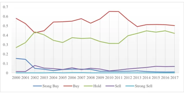
Figure 2: Distribution of Analysts’ Recommendations over time period 2000 to 2017 ... 36
Figure 3: Cumulative Abnormal Returns (CAR) of Recommendation Upgrades... 47
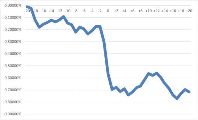
Figure 4:Cumulative Abnormal Returns (CAR) of Recommendation Downgrades ... 48
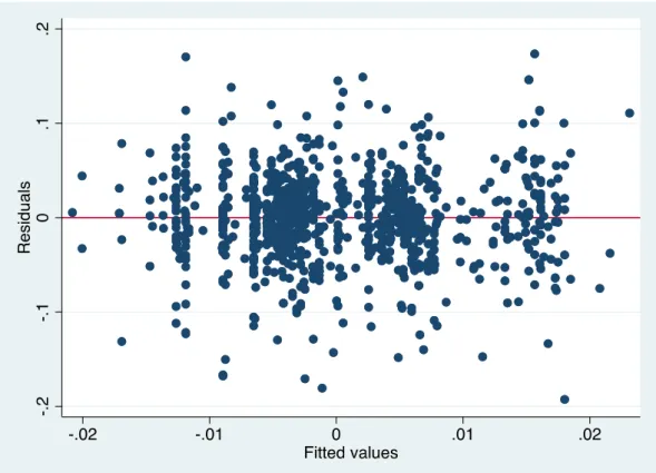
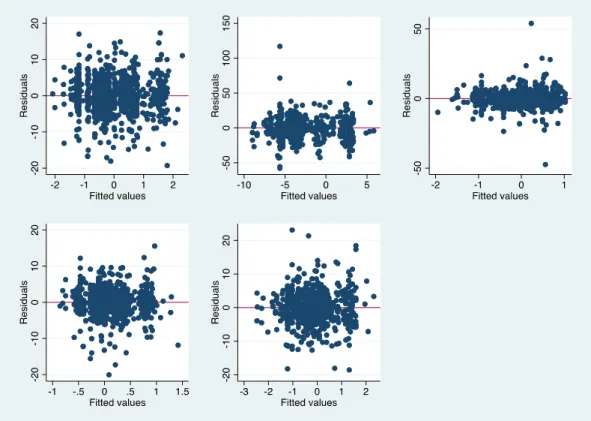
Figure 5: Residuals versus fitted values of the regression model using CAR(-5, +120) ... 52
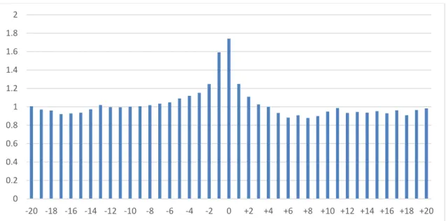
Figure 6: Abnormal Trading Volume, upgrades ... 63
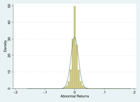
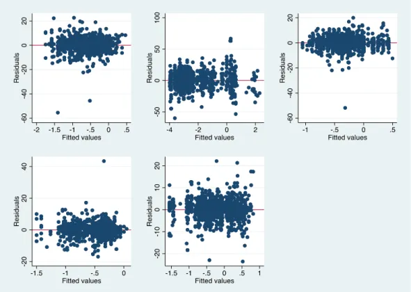
Figure 7: Abnormal Trading Volume, downgrades ... 63 Figure 8: Histogram Abnormal Returns with Normal Density Curve ... XXII Figure 9: Scatterplot of Residuals against Fitted Values Model 1 to 5 of Buy sample ... XXVIII Figure 10: Scatterplot of Residuals squared against Fitted Values Model 1 to 5 of Buy sample ... XXVIII Figure 11: Scatterplot of Residuals against Fitted Values Model 1 to 5 of Sell sample ... XXIX Figure 12: Scatterplot of Residuals squared against Fitted Values Model 1 to 5 of Sell sample XXIX Figure 13: Breusch-Pagan / Cook-Weisberg test output model which uses CAR ( -5, +120) ... XXX
Figure 14: Graphical inspection of Outliers of Upgrades ... XXXI Figure 15: Graphical inspection of Outliers of Downgrades... XXXI
List of Abbreviations
AAR Average Abnormal Returns
AMSE American Stock Exchange
AR Abnormal Returns
Bps Basis Points
CAAR Cumulative Average Abnormal Returns
CAGR Compounded annual growth rate
CAPM Capital Asset Pricing Model
CAR Cumulative Abnormal Returns
DJIA Dow Jones Industrial Average
EP Earnings-to-price
GBM Geometric Brownian Motion
NR Normal Returns
NYSE New York Stock Exchange
OLS Ordinary Least Squares
PB Price-to-book
R Return
1
1
Introduction
This chapter presents an introduction to the topic and provides an overview of this master thesis. As a starting point the background and the situation in analyzing the investment value of analysts are presented. This section also describes the research question and the subsequent hypotheses.
1.1 Background and Situation
Extant literature has explored analysts stock recommendations extensively and the interest in analyzing analysts for financial researchers is of significant interest as their activities affect capital market efficiency.
Analysts are seen as an important agent between investors and companies they follow and their main tasks are forecasting earnings, writing stock recommendations reports and assisting with their opinions indirectly investment banking trading volumes. Based on their intensive analytical research process, analysts provide buy, hold or sell recommendations to clients, potential investors or to their own asset management departments. Their activities leave space for fundamental questions, for example are analysts able to predict winner stocks and loser stocks? If so, how quickly are information's provided by analysts incorporated in market prices, do analysts have the ability to predict market movements and are analysts assisting markets to move towards efficiency?
According to Grossman and Stiglitz (1980) observations the market does not perfectly incorporate all information's and investors need analysts as market agent, who are able to find overvalued and undervalued securities and keep the markets efficient. Whereas advocates for efficient market hypothesis claim that markets and stock prices reflect all publicly information analysts’ recommendations do not result in any value to investors as stock price movements are unpredictable and they follow a random walk. This view is kind of naive, as the banking sector employs thousands of analysts whose job is to follow corporations in order to collect data, analyze data, and publish reports about earnings,
growth potential, management quality, and to give, based on the analyzing process; buy, hold or sell recommendations; otherwise the huge effort would not be compensated.
Further previous literature, like Sahut (2011) and Mola (2012) confirmed analysts are reducing information asymmetries and their actively monitoring activities tend to reduce the principal-agent problem between managers and outside investors. Sahut (2011) confirms the more analysts are following a corporation, the lower is the information asymmetry and the less volatile are stock returns.
Furthermore, it is common known that sell-side analysts are more reluctant to issue negative recommendations, which is confirmed by several statistical analyses like Stickel (1995), Womack (1996) and Barber, Lehavy, McNichols and Trueman (2001). Reasons for the rareness of negative recommendations is the risk to hurt the investment banking relationship with the subsequent downgraded company and the risk for incorrect sell recommendation is much higher than for an incorrect buy recommendation. Due to the less frequency of negative recommendations, the attention and therefore the after-effect is much higher.
One part of my research is to address the question if analysts’ recommendations have investment value? If the information can be used systematically then it would be possible for investors to get an added value in form of higher performance returns (generate alpha) and analysts must have the ability to find underpriced and overpriced stocks.
My analysis has shown there is a gap in the research in analyzing the performance of recommendations and their investment value, as the most research papers are based on the time period prior to 2000.
3
1.2 Objective and Research Aim
The aim of this broad area is manifold and throughout the scope of this research study, therefore the author seeks to identify empirically, the market impact of analysts' recommendation upgrades and downgrades on the 30 stocks listed in the U.S. Dow Jones Industrial Average Index (DJIA).
The main motivation of this study is to answer the question whether, it is it worth to follow the analysts in the US stock market and if these recommendations are valuable to investors.
In this context, the sample data should provide answers to the following hypotheses:
Hypothesis 1: Analysts are issuing mostly optimistic recommendations and are more reluctant to issue sell recommendations.
Hypothesis 2: Analysts are following large capitalized corporations and are largely covering certain attractive sectors.
Hypothesis 3: Change in recommendations for stocks with low analyst coverage
have a greater positive impact on prices compared to stocks with high analyst coverage.
Hypothesis 4: Analysts are able to add value through finding overpriced and underpriced securities.
Hypothesis 5: Analysts do more upgrades in recommendations when investor
sentiment is high and more downgrades when investor sentiment is low.
Hypothesis 6: Change in recommendations for stocks with high brokerage coverage have a greater impact on prices than stocks with lower brokerage coverage.
1.3 Research Question
This master thesis is based on assessing if sell-side analysts employed by investment banks and brokerage houses have investment value for investors.
Thus, the addressed research question is:
Do Analysts’ Recommendations have Investment Value?
In order to be able to answer the research question of this master thesis, it is imperative to design a clear and structured methodology which is being explained in section three
Research Methodology.
1.4 Overview
The remainder of this empirical master thesis is organized as follows.
Chapter two provides a review of relevant literature on the research areas - analyzing the investment value and the profitability of sell-side security analysts. The selected review contains the most useful approaches in assessing the investment value and profitability of analysts' recommendations.
Chapter three presents the primary data, the rating scale classification and the applied research methodology and its specification in order to conduct the descriptive analysis, to analyze the impact of recommendation revisions on stock prices and the cross-sectional regression analysis.
The fourth chapter aims to response the questioned hypothesis, shows and evaluates the results of the research and chapter five summarizes the findings and discusses some of their implications.
5
2
Literature Review
This chapter presents in chronological order a review of relevant literature, as well as the most important findings regarding how analysts stock recommendations affect stock returns and to which extend investors are able to achieve abnormal returns. Previous research, for example Stickel (1995), Womack (1996), Barber et al. (1998), Barber et al. (2001) and Jegadeesh, Kim, Krische and Lee (2004) have demonstrated in their studies that consensus analysts' recommendations can beat the market and carry investment value.
The content of each summary is based on each academic publication and the quotations are declared underneath each summary.
2.1 Recommendation Research before and during 1980s
The first academic research paper with the title "Can Stock Market Forecasters Forecast?" in assessing if security analysts can beat the market with their recommendations was conducted by Alfred Cowles in 1933.
The paper is divided into two parts, the first part analyses the forecasting ability regarding superior returns of 20 fire insurance companies and 16 financial services during the sample period ranging from 1928 to July 1932, while the second part deals with the ability to predict future stock price levels, forecasted by 24 financial publications. Cowles finding was that some 7500 recommendations on stocks did not outperform the market and neither achieved abnormal returns and no specific investment skills were present. The same poor performance was confirmed for the forecasting ability of the future stock market movements from publications like the Wall Street Journal. A significant impact for the underperformance can be related due to the exogenous effect of the great crash in 1929 and their after-effect. According to Michaely and Womack (2002a) the underperformance could be a result of Cowles incorrect computation and a misstated understanding of benchmark investing during this time.
No further research was in the field of analysts' recommendations forecasting ability existent until the 1970s.
In 1986 Elton, Gruber and Grossman examined with a first comprehensive database the period from 1981 to 1983 consisting of 720 analysts from 33 brokerage firms. The paper titled, "Discrete Expectational Data and Portfolio Performance" focus was mainly on large capitalized corporations, which had a minimum coverage of three analysts. The study analyzed the monthly impact of recommendation changes, upgrades (from a lower to a higher rating) and downgrades (from a higher to a lower rating). Descriptive summary statistic for the sample shows a recommendation distribution of 48.00% buy and just 2.00% of sell recommendations. Beta-adjusted returns delivered for both scenarios insignificant excess returns. Upgrades, accumulated in the month after the recommendation release abnormal returns of 3.43%, while downgrades resulted in negative excess returns of -2.26%.
Drawback of the study is, that the calculation of beta-adjusted returns is based on a monthly basis one month after the recommendation announcement and therefore the real impact of the recommendation change on returns is unclear.
(Elton, et. al., 1986)
2.2 Publications 1994 - 1999
Following publications differ to Elton et. al., (1986) approach, as these studies are based on a larger scale database and the calculation of abnormal returns is based on a daily basis, to capture the immediately impact of recommendation announcements on stock prices and their returns.
"The Anatomy of the Performance of Buy and Sell Recommendations" analyzed the short-term and long-term price performance of 8,790 buy and 8,167 sell recommendations from the financial data source Zack, which obtained written recommendation reports from brokerage research departments. This research was based on a unique database covering the period 1988-1991, on 1,179 covered stocks, made by
7
Stickel's (1995) study contributes to the existing literature, as the focus is on the determinants of stock performance on those stock recommendations and by the use of a cross-sectional analysis. With a cross-sectional regression analysis, six hypotheses were tested in order to identify which factors contribute most to the stock price performance of those buy and sell recommendations.
Following factors were in the multiple regression analysis included:
- The recommendation strength
- The size of the recommendation change, by how much it skips ranks
- Analyst reputation
- Number of employed analysts per brokerage firm and
- The difference in the market capitalization of those covered equities.
The uncertainty if a recommendation was announced before or after entering Zacks database was taken into account through ±5-day time window. In total, Stickel (1995) observed 21,387 recommendation changes, with a frequency distribution of 55% buy, 33% hold and 12% sell recommendations.
Buy recommendations contributed with a mean of 1.16% to a price increase, while sell recommendations led to an average decline of -1.28% in the time window ±5 day, centred on the recorded recommendation date by Zacks.
(Stickel, Scott E., 1995)
Womack's (1996) research with the title "Do Brokerage Analysts Recommendations Have Investment Value?" contributes to the academic literature as the paper examines how stock prices and volumes react to changes in analysts' recommendations.
In order to examine his analysis Womack collected the data from First Call, a database, which collected real-time recommendations directly from the majority of US and international security firms and provided access to this data to investors through an on-line PC system. Years ranging from 1989-1991 were studied in the research with a focus on a narrow sample by examining the recommendations of the fourteen major U.S. brokerage firms. With the focus in analyzing the stock recommendations of 14 brokerage research departments, the author aimed to control the immediately availability of their research reports to institutional investors and investment managers.
Womack's study is based on a database of 1,573 changes in analyst recommendations from strong buy to strong sell, or from strong sell to strong buy, made on 822 different companies. Womack examined analyst’s recommendation changes by dividing the sample of 1,573 recommendation changes into four categories: added or removed stocks from the most favorable category buy or added or removed stocks from the least favorable category sell.
The remarkable result to emerge out of the authors sample data is that the majority of the analysts’ recommendations were issued on large-capitalization companies, while just 10% of the recommendations are recommended on small-capitalization companies. Further was examined the category added to buy contains significantly most of the recommendations, than added to sell category. Which also is a significant evidence that analysts are more reluctant to issue sell recommendations. Womack's results show significant price reactions for stocks added to buy and for stocks added to sell. The price for stocks added to the buy list increased on average in the 3-day time window by 3.00%, while the stocks added to the sell category declined on average by -4.70%. The results are adjusted for size, industry and by using the Fama-French three factor model. Further, he provides evidence that stock prices after recommendation changes move significantly towards analysts forecasted recommendation direction. After the recommendation release, upgraded stocks added to buy drift on average by 2.4% which holds up to three months, while downgraded stocks added to sell drift over a six-month period on average by -9.1%. Similarly, to Barber et. al. (1998), recommendation changes on small-capitalized companies caused a larger market movement, compared to recommendation changes on large-capitalized companies. Decomposition of the post-recommendation drift shows excess returns are not mean reverting and the market movement towards analyst’s recommendation direction does not appear to be short lifted.
Womack's findings give compelling evidence that analysts recommendation changes significantly influenced stock prices.
(Womack, Kent L., 1996)
The published academic paper by Barber, Lehavy, McNichols and Trueman, "Can investors profit from the prophets? Consensus analyst recommendations and stock returns" build the fundamental basis in the question of the profitability of
9
This analysis is based on a unique database provided by the Research Investment database Zack, which encompasses over 360,000 recommendations, issued from 269 brokerage houses, provided from 4,340 analysts over the time period 1986 to 1996. The recommendation frequency of the database excluding recommendations with termination of coverage showed a distribution of 54.0% of buy recommendations, 39.5% of hold and the minority of 6.3% of sell recommendations respectively.
By building calendar time portfolios and classifying the covered firms according to their average ratings into five portfolios, where the first portfolio consists of the most highly recommended stocks, for which the rating Ai,t-1is in the scale 1 ≤ Ai, t-1 ≤ 1.5 and the fifth portfolio with a rating scale Ai, t-1 ≥ 3 contains the least recommended stocks. This approach follows the rating scale, rating (1) a strong buy, (2) a buy, (3) a hold, (4) a sell and (5) a strong sell recommendation. The returns are then calculated for each portfolio after the close of the trading day. The daily value-weighted returns Rp,tfor each portfolio
p on each day t, are then further compounded to a monthly return. The next step involves the calculation of market adjusted-returns by taking the difference of the monthly portfolio return and the monthly return on a value-weighted market index. As the portfolio classification technique rebalances the portfolio after the close of the trading day, the return calculation uses the similar approach and calculates monthly-adjusted returns by excluding first-day return to analysts’ recommendations. This approach takes into account that investors cannot act before any research reports are made public.
The results showed over the sample period a significant outperformance of the most highly recommended portfolio by an annualized geometric mean of 18.8% while the least recommended portfolio returned on average just 5.78%. The outperformance of the most favorably recommended stocks is even persistent after controlling for Fama-French factors and momentum factors, were a positive excess return of 4% per year was achieved, while a negative annually excess return of 5% was earned by the least favorably recommended stocks. In the end, the results are most pronounced for small and medium sized companies. This strong evidence justified the ability of research departments to transfer the costs of intensive security analysis into superior returns for their investors.
Limitation of the paper is that the calculation of the outperformance in based before deducting transaction costs.
(Barber et al., 1998)
"How Do Stock Markets Process Analysts' Recommendations?" by Juergens (1999) provides evidence to the question whether analysts’ recommendations have investment value. The primary data used was gathered from the same data source as Womack's (1996) research is based on. 3,679 recommendations for over 208 firms in the sector computer or computer-related firms were analyzed in the sample period 1993 to 1996.
The author contributes to the literature as the analysis is based on all types of recommendations, while Stickel (1995) Womack (1996) analyzed only changes from the most highly recommended stocks and changes from the least recommended stocks. Further it differs by analyzing the impact of analysts' recommendations and public announcements on daily and on intraday returns.
Summary statistic shows for the period ranging from 1993-1996 a dramatically increase in the number of firms covered by analysts and an increase in the total number of recommendations. In line with findings from Stickel (1995) and Womack (1999) her sample contains the similar recommendation frequency distribution, as the sample exits of 56% positive recommendations and 3% of sell recommendations. These findings provide again evidence that analysts are more reluctant to issue sell recommendations. The same can be concluded from a 5 x 5 recommendation change matrix, as most of the recommendations are centered in the upper part. Looking on abnormal returns confirm the ability to outperform the market by following analysts’ recommendations. Remarkable cumulative abnormal returns (CAR) were achieved by recommendation changes from hold to strong buy upgrade which resulted into a 3-day CAR of 4.14%, which is of greater magnitude then found in previous studies.1 In contrast a downgrade change from strong buy to hold earned on average a negative CAR rate of -5.39%. All positive recommendations have earned on average a 3-day CAR of 1.91%, while all negative recommendations garnered a negative return of -3.14%. Significantly return
11
difference was further confirmed with a mean difference test. The market impact of analysts' recommendations was further assessed by intraday return calculation. Intraday returns were calculated for 15-minute intervals in the time frame, two hours before and two hours after the recommendation announcement. The results were significant at the 1% significance level for positive recommendations (0.55%) and negative recommendations earned -1.27%.
To conclude Juergens analysis confirmed, it is possible to earn significant intraday returns with analysts' recommendations and those reports provide investment value around the recommendation announcement time.
(Juergens, 1999)
2.3 Publications 2000 - 2010
Barber et. al. research paper "Prophets and losses: Reassessing the returns to analysts' stock recommendations" continues on his previous research (1998) where analyst’s recommendation has significantly outperformed those recommendations of the least recommended stocks throughout the time period 1986-1996.
His subsequent paper aims to validate if the outperformance is still present during the narrow time frame from 1996 to 2000, where it was widely spread analysts were working in favor of investment banking activities and writing research reports in favor for companies which are having a client relationship with the investment bank. A total of 160,000 recommendations were collected from Thomson Financial' s database First Call, made by 299 securities firms, covering 9,621 companies. Breaking down the total number of recommendations, the sample contains overall of 67.9% of strong buy/ buy, 29.1% of hold and 3.0% of sell/ strong sell recommendations.
The analysis follows the approach of Barber et al (1998), where the covered firms are based on their average ratings, placed into five portfolios on a calendar time basis. Analysts buy recommendations have on average significantly outperformed those of least favorable recommendations during 1996-99, while on the contrary this outperformance
vanished in the year 2000 regardless of the market phase and of the sectors of those recommended stocks. The most highly recommended stocks returned on average annualized excess return of -31.20%, while the market-adjusted return for the least recommended stocks averaged an annualized return of 48.66%. This unpredicted pattern and the huge dispersion between both portfolio performance raises questions over the usefulness of the investment value of analyst’s stock recommendations in the long-term. There is still considerable uncertainty if the year 2000 is a turning point in the usefulness of analysts’ accuracy and if this is caused by increasing incentives to forecasting towards investment banking benefits.
(Barber et. al., 2001)
In 2004 Barber et. al. expanded his analysis of security analyst’s investment value by, investigating in his publication “Comparing the stock recommendation performance of investment banks and independent research firms”, the profitability of security recommendations issued from independent research firms and investment banks, for a narrow sample window during the period 1996 to 2003.
The conducted study collected the data from Thomson Financial' s First Call database and the data sample encompassed 335,000 recommendations issued by 409 securities firms.
This paper divides analysts’ recommendations into two samples, issued by independent research firms (without any investment banking activities) and issued by investment banks. It further divides the sub samples, according to their ratings into two sub portfolios, first portfolio with buy recommendations and second portfolio with hold and sell
recommendations.
By using the Fama-French Method and controlling for market risk, size, book-to-market and price momentum effects, the daily abnormal returns were calculated for each portfolio respectively.
A further analysis was conducted by splitting the time period into two market phases, time frame until March 10, 2000 refers as the bull market and following to that date as
13
The sample of investment banks buy recommendation is further broken down into three investment banking categories in order to investigate if a performance difference exists between sanctioned and non-sanctioned investment banks.
The results confirm the hypothesis that investment banks are more reluctant to downgrade stocks, as the findings showed investment banks are not able to outperform buy recommendations of independent research firms. The buy portfolio of independent research firms has outperformed by 3.1 basis points (bps) on a daily basis or by 8% yearly. On the other hand, the hold and sell portfolio of investment banks has outperformed by -1.8 bps per day and annualized by -4.5%, those recommendations of independent research firms. These results conclude by following the sell recommendations of investment banking research, investors are able to minimize their financial losses.
Investment banking buy recommendations have on average outreached those of independent research firms, by a statistically insignificant 0.4 bps in the bull market. While in the bear market independent research firms buy recommendations have exceeded significantly those of investment banks by 6.9 bps on a daily basis and more than 17% annually. The market phase analysis further confirms, investment banking hold and sell recommendations are able to outperform independent research firms, as the results showed the majority of their hold and sell recommendations are concentrated in the bear market and outperformed those of independent research firms by 3.5 bps per day.
The performance analysis between the three investment banking categories, with the group sanctioned investment banks2 (containing of 10 banks), non-sanctioned investment banks (which are lead underwriter like the 10 sanctioned banks) and non-sanctioned banks (with no active lead underwriter role, which are syndicate members) showed, there is no difference among the performance of sanctioned and non-sanctioned investment banks compared to independent research firms. All three categories were not able to outperform those buy recommendations of independent research firms and do not show evidence that non-sanctioned banks provide independent research reports to investors. Conflict of interest claims of sell side analysts are supported by Barber et. al. results.
(Barber et. al., 2005)
Years ranging from 1985-1998 were studied in the research published by Jegadeesh, Kim, Krische and Lee in “Analyzing the Analysts: When do Recommendations Add Value?” with a focus finding out the source of investment value those recommendations provide. As a primary data source Zacks Investment Research database was used.
Recommendation level and changes in recommendations were analyzed by using twelve characteristic variables, which have the ability to predict returns as confirmed by previous literature and previous studies.
These twelve explanatory variables are categorized into five categories: (1) Momentum and Trading Volume;
(2) Valuation Multiples; (3) Growth Indicators; (4) Firm Size and
(5) Fundamental Indicators.
As these twelve variables are correlated with future returns, Jegadeesh et. al. expected, a correlation towards the same way with recommendation level and changes.
The hypothesis of this study is, if analysts are paying attention to these variables in the above-mentioned categories, then most recommended stocks must be based on following characteristic:
• High momentum stocks and / or low volume stocks;
• High valuation with a high earnings-to-price ratio (EP) and high book-to-price ratio (PB);
• Low past growth and low expected future growth or
• Low accruals ratio and low capital expenditure ratio.
Recommendation level is calculated as an average of all outstanding recommendations within one calendar year, while the recommendation change is calculated as the difference between the current calendar quarter and the prior calendar quarter, which results either in an increase or decrease in the consensus level of analyst recommendation.
15
This study used descriptive statistic, by analyzing on a firm level the sample distribution across years. The results show a remarkable increase in firm observations over time and yields over 56 quarters an average of 971.4 firm observations per quarter. A further descriptive analysis was conducted on the analyst’s sample recommendations. Consensus recommendation levels and recommendation changes were grouped into quintiles, where the quintile 0.00 contains the least recommended stocks and the quintile 1.00 contains the most recommended stocks. The outcome of the five consensus recommendation level quintiles, are in line with other studies and confirm clearly, analysts are more reluctant to issue sell recommendations. On the other hand, the results of the recommendation changes quintiles, show firms were more likely to be downgraded than upgraded by analysts.
Positive correlation between future market-adjusted returns and recommendation level and changes was examined by using the Spearman rank correlation method and the results give evidence for analyst’s predictive ability in stock recommendations. The Spearman rank correlation was further used for assessing the correlation between future returns and the twelve investment variables. The findings confirmed a correlation between the explanatory variables and future returns. The variables positive price momentum, positive earnings momentum, and total accrual ratio were in 75% of the quarters presents and were identified as the most predictive variables with the ability of causing positive future returns. The Spearman correlation analysis between consensus recommendation level and changes in recommendation with the twelve defined investment variables, demonstrated a strong positive correlation with momentum factors. This implies analysts most favorably recommendations are based on securities with momentum factors. Further analysts prefer high turnover stocks, low PB, high EP, high past growth and high expected future growth as well stocks with a high accruals and high capital expenditure ratios. Analysts preference for momentum stocks, was further confirmed by using a multivariate regression analysis, with analyst’s recommendation as the dependent variable and the twelve investment variables as explanatory variables.
Summarizing up Jegadeesh et al. examined analysts’ recommendations as well the twelve considered investment variables, have the ability to predict future returns. A positive
relation exists for analysts’ recommendations and explanatory variables, where the most striking focus is on momentum stocks with a strong past performance which is expected to continue in the future. Although the authors showed that most recommended stocks have outperformed least recommended stocks.
(Jegadeesh et. al., 2004)
2.4 Publications 2011 - 2016
Souček and Wasserek (2014) study uses as a primary data source Thomson Reuters
I/B/E/S database and the analyzed period ranging from 2000-2012, with a focus on the German DAX 30 Index. Based on a sample of 12,998 observations, made by 1,446 from 126 security firms, the aim of the paper is to study the impact of analysts’ recommendation upgrades, downgrades and reiterations on the stock returns and if investors are able to profit from those recommendations.
Souček et. al. contribute to the academic literature as this study is the first research on analysts’ recommendations on the German DAX and for a more recent time frame. In addition, the paper analyses compared to Stickel (1995) and Womack (1996) the price reactions of all recommendations.
Excess return calculation is based on the approach of the famous theoretical Capital Asset Pricing Model (CAPM) and controlling of other factors and to test the robustness, the Fama-French (1997) three factor model, as well the Carhart (1997) four factor extension model was applied.
The recommendation sample contains 41.7% of buy recommendations, 39.1% of hold and surprisingly a large amount of 19.2% sell recommendations. This gives evidence that the analysts’ recommendations frequency distribution is compared to the US findings less biased. Recommendation change, 5 x 5 transition matrix shows the bulk of recommendations are in the upper 3 x 3 part and illustrates clearly that sell recommendations are less frequent than buy recommendations.
17
Recommendation changes to upgrades accumulated significantly positive abnormal returns around the recommendation release date, while recommendation downgrades accumulated significantly negative returns. The same return patterns apply for initial recommendations, a new buy recommendation gains significantly positive returns, whereas significantly negative returns hold and sell recommendations accumulate. No statistically significant returns and market reactions were obtained by recommendation reiterations. Further as confirmed from previous papers, the paper provides evidence that the stock market reaction on recommendation revisions is most powerful at the announcement day and the post-recommendation drift in stock prices last up to six months for upgrades and four months for downgrades. Due to the findings that the stock market reaction is strongest at the recommendation release date, the analysis give further evidence that investors are able to gain the highest profit from analysts’ recommendations by trading on the event day in a timely manner.
(Souček et al, 2014)
Years ranging from 1996 to 2012 were analyzed by Boulland, Ornthanalai and Womack in the research paper "Speed and Expertise in Stock Picking: Older, Slower and Wiser?" with the aim to examine how the speed of recommendation changes have investment value. The study contributes to the literature as it is one of the first study that examines the impact of analyst’s decision speed-style on the stocks, analysts are following and by looking on the investment value by classifying analysts into two types according to their speed.
The final sample for the period 1993 to 2012 uses I/B/E/S database, which contained 240,957 observations. Overall the sample contains solely recommendation changes, upgrades (44.54%) and downgrades (55.46%).
Descriptive statistic for the sample shows an average of a recommendation stay without a change is 12.36 months and analysts are following on average 6.91 stocks.
The paper calls the time or the speed it takes to revise analyst’s recommendation as turnover. Further analysts can be classified into two categories, fast-turnover analysts, who change their recommendations on average every 6 months and slow-turnover analysts who typically change their opinion approximately every 20 months. The study
uses Barber et. al. (2001) famous real-calendar time portfolio approach, which is in the academic literature the standard approach in assessing abnormal returns of buy vs. sell recommendations. Boulland et. al. found that recommendation changes made by slow-turnover analysts have significantly outperformed by 1.93% in the first five months after the recommendation change, relative to fast-turnover analysts. While risk-adjusted returns of downgrades are by 1.23% relatively lower. A multivariate regression analysis, with analysts' recommendation speed-style as the dependent variable and various analyst’s characteristics as independent variables delivered strong evidence for the relation between analyst’s ability to make better recommendations and their decision-speed. The coefficients of analyst’s characteristic variables top brokerage house, experience and analyst’s all-star category have significantly negatively effects on the dependent variable fast-turnover group, further indicates slow-turnover analyst’s ability to make more careful and better decisions. In summary, the paper demonstrates better recommendations are made by slow-turnover analysts and those add value for investors through their prudent decision style.
19
3
Research Methodology
This section provides information about the methodology by explaining the database, the time period of the analysis, the selected equity index, the rating scale classification and the research design.
3.1 The Data Selection
The analyst recommendations used in this study were obtained from the financial data provider Bloomberg. The recommendation time frame encompasses the period 2000 to 2017 with a solely focus on the Dow Jones Industrial Average Index (DJIA). One of the significant reason for choosing the DJIA, is as it shows the performance of the industrial sector within the American economy and contains the 30 largest and mainly important publicly owned companies based in the United States. The companies listed in the DJIA, are attached in table 10 in the Appendix.
The recommendations had to fulfil some criteria to be included in the entire data sample:3
- At least one analyst who has issued a recommendation on a specific stock and reconsidered the opinion within 365 days. If a recommendation exceeds the time window of 365 days, it will be seen as a new recommendation, in order to avoid outdated recommendations with no reference to previous one.
- Recommendations issued when the American Stock Exchange (AMSE) and the New York Stock Exchange (NYSE) is closed are eliminated to ensure availability of stock returns on all trading days, as the DJIA is quoted at the end of every US trading day.
Consequently, to create the sample of recommendation upgrades and downgrades the following criteria were additionally imposed for the sample to be used in the event study and cross-sectional regression analysis:
- Recommendations are excluded if an analyst makes only one recommendation, as those recommendations have no reference to change in recommendations.
3Criteria selection follows the approach by Stickel (1995), Jegadeesh et al (2010) and Souček et al
- Recommendation revisions of previous recommendations are excluded, since recommendations on securities issued by the same analysts are classified as upgrades or downgrades compared to the previous announced recommendations.
In the event study and cross-sectional regression analysis, buy recommendations are defined as all rating upgrades to a strong buy and buy coming from a recommendation of hold, sell or strong sell. Sell recommendations are defined as all downgrades in recommendation revision to strong sell and sell, coming from a rating of strong buy, buy or hold. Including recommendation downward revisions to hold from a strong buy or a buy recommendation.
All recommendations which are present the first time in the data sample, are treated as recommendation initiation. This might be not the true initiation of coverage. This assumption is relevant in order to start with the analysis.
The stock prices data will be looked up on Bloomberg. For all 30 DJIA securities the official daily closing price is chosen, after the adjustment of capital market events like stock-dividends, dividend pay-out and mergers and acquisitions. For each security, the corresponding stock price return is calculated as the natural logarithm difference in the closing price over the one day period as follow:
𝑅𝑡 = 𝐿𝑛 [ 𝑃𝑡 𝑃𝑡−1]
This approach is the most acceptable method in finance to model asset prices and the main benefit of using log-returns instead of arithmetic returns in modeling assets prices is to avoid the occurrence of negative assets prices, as asset prices never take prices less than zero. Since in academic finance the process of a stock price St at time t is modelled
as a stochastic process, which is called geometric Brownian motion (GBM), a further advantage is the assumption of normally distributed log-returns. This can be opposed as the price of a security follows a GBM (Hilber, 2017).
21
3.2 Rating Scale
‘Buy’, ‘hold’ and ‘sell’ are the most commonly used and known expressions by security analysts. However, from broker to broker houses analysts use slightly different expressions for the same meaning, for example ‘attractive’, ‘neutral’, ‘market-perform’ or ‘underweight’, see table 11 in Appendix.
As the sample consists of 131 different rating expressions as the individual brokerage firms use a variety of different rating phrases for their stock recommendations, all expressions have to be analyzed and standardized and coded into a common rating system.
To ensure comparability of recommendations across brokerage firms, the study make use of the common 5-point scale rating system. The different analyst’s recommendations were classified into a common rating scale from 1 to 5. Where rating 1 is a ‘Strong buy’, 2 is a ‘Buy’, 3 is a ‘Hold’, 4 is a ‘Sell’ and 5 is a ‘Strong sell’. Rating 6 ‘No coverage’ was attached when the analyst coverage was terminated.
Some expressions contain two rating phrases, a firm and an industry recommendation separated by a slash. The used rating expression in this analysis, is solely the firm recommendation, which is the text before the slash.
3.3 Research Design
It is imperative that this study requires mainly quantitative analysis in extent to answer the addressed research question. The methodology of this master thesis will consist of different steps.
The first step will be the review of all recommendations in the sample period and standardizing the expressions into a common rating scale, by attaching numerical numbers to all recommendation expressions. Subsequently, the data sample will be analyzed by applying descriptive statistics on all recorded recommendations exported from Bloomberg. Proceeding with the analysis, only changes in recommendations are
used, which means any revisions of previous recommendations are excluded. Continuing the impact of recommendation changes on stock prices will be analyzed by applying the methodological concept of an event study. The last step conducts a cross-sectional regression analysis to determine the performance of recommendation revisions.
3.3.1 Descriptive Statistics
To begin with the quantitative analysis, the entire data sample will be analyzed by using descriptive statistics.
As a first step, a table with annual descriptive statistics which include per year the number of firms covered, number of analysts and number of brokerages, which should give information’s about the annually average number of analysts covering firms and average number of analysts employed at a brokerage house, as well the average number over the entire sample period.
Secondly, I will analyze the frequency distribution of the recommendations classified among three rating categories buy, hold and sell. Whereas category buy encompasses strong buy and buy recommendations and the category sell encompasses sell and strong sell recommendations.
Thirdly descriptive statistics of analysts' recommendations is going to be conducted for each DJIA firm separately. Descriptive statistics for each firm aims to break down the number of analysts following a company, number of brokerages per company and the average rating for each firm and their median respectively. The motivation is to find out, if brokerage houses tend to cover the top level of large capitalized firms, if a specific sector is attractive to follow and for which firm analysts are issuing most highly (least) recommendations.
Finally, all possible changes in analysts' recommendations are going to be examined with a 5 x 5 recommendation change matrix. The purpose of the matrix is to show where the bulk of recommendations are clustered and to deliver the number of upgrades and
23
downgrades. The matrix will give insight if more upgrades or downgrades occurred in the encompassing sample period.
3.3.2 Event Study and Cross-Sectional Regression Analysis
The quantitative analysis in assessing the price performance of analysts’ recommendations will be examined by the usage of the commonly known event study concept and a cross-sectional regression analysis. This master thesis builds upon the event study methodology, which is widely accepted and was applied in previous literature, like Fama, Fisher, Jensen and Roll (1969), Stickel (1995), Womack (1996) and Souček et al. (2014).
The event study methodology is used to investigate the share price reaction following the recommendation changes. The methodological approach used in this master thesis follows the event study methodology described by Bowman (1983). This methodological concept is also known under the names such as residual analysis and abnormal performance index tests.
To start with an event study, the structure of an event study involves the following steps, according to Bowman (1983) and De Jong (2007) described structure of an event study:
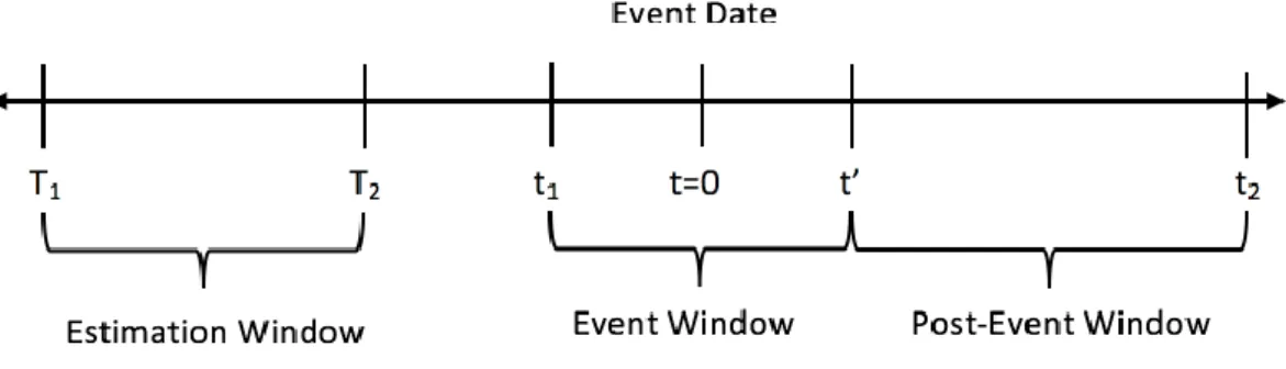
I. Identify the event of interest and precisely the timing of the event.
The event of interest in this master thesis is the investigation of recommendation revisions, which occur for different securities at different calendar dates. To begin with, the timing of the event has to be identified. The timing of the event equals to the exact announcement day of the recommendation as recorded by the Bloomberg database. Consequently, all different calendar dates of all single events need to be standardized to event time zero (𝑡 = 0), as the aim is to bring all single events together into a single sample. This event time procedure allows to describe time periods in event time relative to the zero time when the event, the recommendation revisions occurred. The figure below shows the time line of an event study.
Figure 1: Time Line of an Event Study.
In this study, the time period of the estimation window right before the event window ranges from 𝑇1 = −180 𝑡𝑜 𝑇2 = −40, following the length of the estimation window
from Brown and Warner (1980) classical event study paper. The information content event window in the analysis was expanded to include days before the announcement date, due to the uncertainty of the announcement date of the analysts’ recommendations. This encounters the likelihood that an investment bank or brokerage house research departments informs specific target clients on any recommendation changes prior to the date of the research report and prior to the announcement date in the Bloomberg database. According to the Ethical and Professional Investment Standards of the CFA Institute (2017) all clients of an investment bank or brokerage house must have a fair chance to act on every recommendation, nevertheless following the guidance it is acceptable to communicate any recommendations to clients first who pay for a different service level. Therefore, it is useful to extend the event window around the event date to capture a pre-event drift before the actual announcement date. The chosen pre-event period ranges from
𝑡1 = −20 𝑡𝑜 𝑡2 = +120 and follows the time line structure of two event studies, as
Stickel (1995) showed, a pre-event drift occur twenty days before the event and Womack (1996) findings showed the post-event drift might last up to 6 months after the event.
II. Calculate normal returns based on a specified benchmark model for normal share price behavior in order to assume the event had not taken place.
The second step requires the specification of an appropriate benchmark to calculate and model normal stock return behavior. The S&P 500 Index is used as a benchmark index,
25
since the S&P 500 includes all stocks tracked in the DJIA index and the S&P 500 is one of the broadest benchmark index which tracks the 500 largest US corporations. The selection of the S&P 500 as a broad index in this study to represent the market portfolio aligns with Womack and Zhang (2003) suggestions to select either the S&P 500 or the Russell 2000 index.
Next step requires the selection of a statistical model to calculate the residuals of the process generating returns. Referring to Bowman (1983) the correct model is a critical element in event studies to be able to find security price reactions. In this study, the widely accepted single factor model, called market model is chosen:
𝑅𝑖𝑡 = 𝛼𝑖+ 𝛽𝑖𝑅𝑚𝑡+ 𝜀𝑖𝑡
where the parameters are as follow, Ritis the return on security i in period t, Rmt is the
return on the market portfolio, the selected market benchmark in period t, coefficients 𝛼
and 𝛽 are constants for security i. The coefficient beta 𝛽𝑖 or slope of the regression,
measures the sensitivity of return Rit with the reference market and returns have to be
adjusted for differences in beta, since the market sensitivity for each stock is not equal to one. The parameter 𝜀𝑖𝑡 is the error term or residual of the market model, which is completely a random part of the model.
The calculation of normal returns is performed over the estimation period ranging from the start 𝑇1 = −180 up to the end 𝑇2 = −40. From the above model, normal returns can be mathematically derived as follows:
𝑁𝑅𝑖𝑡 = 𝛼̂𝑖 + 𝛽̂𝑖𝑅𝑚𝑡
Subsequently the parameters of the model are estimated by using Ordinary Least Squares (OLS) regression method. The next step involves the calculation of residuals based on the estimated parameters 𝛼̂𝑖 and 𝛽̂𝑖. This means abnormal returns can be expressed as residuals or error terms of the market model:
𝜀̂𝑖𝑡 = 𝑅𝑖𝑡− (𝛼̂𝑖𝑡 + 𝛽̂𝑖𝑡𝑅𝑚𝑡)
According to Bachmann (2015a) and (2015b) residuals expectation and OLS estimation assumptions are the following:
𝐸(𝜀𝑖𝑡) = 0 𝑓𝑜𝑟 𝑖 = 1, … , 𝑁
This means on average the expected value of abnormal (excess returns) has to be zero and holds in an efficient market environment, where no excess returns can be achieved. This means any non-zero value in residuals is termed as abnormal (excess) returns, since the expected value of the residuals is assumed to be zero on average, according to the above equation.
The second property states a zero correlation, as it is assumed the error term is not correlated with the market return Rm and security return Rit is uncorrelated with security
return Rjt. This property is also referred as no autocorrelation in residuals, see Bachmann
(2015f).
𝜎(𝜀𝑖𝑡, 𝜀𝑗𝑡) = 0 𝑓𝑜𝑟 𝑖, 𝑗 = 1, … , 𝑁 𝑎𝑛𝑑 𝑖 ≠ 𝑗
Last required OLS estimation assumption is homoscedasticity, which means all error terms have the same variance.
𝑉(𝜀𝑖) = 𝜎2 𝑓𝑜𝑟 𝑖 = 1, … , 𝑁
This assumption is violated if the variance of the error terms is not constant and depends on the values of the independent variables used in the regression model, referred as heteroscedasticity. Consequently, a violation of the assumption means that the OLS standard errors 𝑠𝑏𝑜, … , 𝑠𝑏𝑘are incorrect and could be either too low or too high.
A graphical inspection, by the usage of residual plot helps to detect whether outliers and heteroscedasticity is present. This approach is of limited use as these residual plots do not provide evidence of that problem. Therefore, it is necessary to conduct statistical tests.
27
Statistically, heteroscedasticity can be assessed by running a Breusch-Pagan test or a White test. The Breusch-Pagan test runs under the following hypothesis:
𝐻0: 𝑐𝑜𝑛𝑠𝑡𝑎𝑛𝑡 𝑒𝑟𝑟𝑜𝑟 𝑣𝑎𝑟𝑖𝑎𝑛𝑐𝑒 𝜎2
𝐻1: 𝑒𝑟𝑟𝑜𝑟 𝑣𝑎𝑟𝑖𝑎𝑛𝑐𝑒 𝑑𝑒𝑝𝑒𝑛𝑑𝑠 𝑜𝑛 𝑝𝑜𝑝𝑢𝑙𝑎𝑡𝑖𝑜𝑛 𝑟𝑒𝑔𝑟𝑒𝑠𝑠𝑖𝑜𝑛 𝑓𝑢𝑛𝑐𝑡𝑖𝑜𝑛 𝐸(⟨𝑦𝑖|𝑥𝑖1, … , 𝑥𝑖𝑘⟩)
The Breusch-Pagan test requires the estimation of the so-called auxiliary regression 𝑒𝑖2 = 𝑎0+ 𝑎1𝑦̂𝑖+ 𝑢𝑖. Consequently, by the use of a chi-squared test statistic it can be decided whether to reject the null hypothesis or not if:
𝑛 ∗ 𝑅2
𝑒2 > 𝜒21,𝛼
where𝜒21,𝛼 is the critical value of a chi-square distribution with 1 degree of freedom and confidence level𝛼. (Bachmann, 2015e)
III. Calculate abnormal (excess) returns in the determined event window.
Step three involves the calculation of abnormal returns, where abnormal returns (AR) are calculated as actual returns (R) minus normal returns (NR) in the event window ranging from t1 to t2.
𝐴𝑅𝑖𝑡 = 𝑅𝑖𝑡− 𝑁𝑅𝑖𝑡
Where Rit is the return on stock i on day t and NRit is defined as the expected return in the
estimation period. The determination of abnormal returns is performed over the event window ranging from 𝑡1 = −20 to 𝑡2 = 120 and the event date is labelled in event time as 𝑡 = 0,as outlined in the first step. Therefore, ARi0 represents abnormal return on the
Due to the fact that there are multiple events4 for each firm present, the relative events are treated as if they belong to separate firms. Assuming the used sample is of size N, a matrix of abnormal returns can be constructed in the following form:
[ 𝐴𝑅𝑖,𝑡1 … 𝐴𝑅𝑁,𝑡1 ⋮ … ⋮ 𝐴𝑅1,−1 … 𝐴𝑅𝑁,−1 𝐴𝑅1,0 … 𝐴𝑅𝑁,0 𝐴𝑅1,1 … 𝐴𝑅𝑁,1 ⋮ 𝐴𝑅𝑖,𝑡2 … … ⋮ 𝐴𝑅𝑁,𝑡2]
Each matrix column presents a time series of abnormal returns for stock i, where the time index t is counted from the event date (t=0). Each row builds a cross-section of abnormal returns for each time period.
Proceeding with the analysis, abnormal returns need to be organized and grouped into two portfolios, either buy or sell portfolio according to the relative event if it is either an upgrade or downgrade in the recommendation revision.
Subsequently the abnormal returns are averaged to improve the information content of the analysis over the observations together. Below equation expresses average abnormal returns (AAR) at time t across all observations under studies.
𝐴𝐴𝑅𝑡 = 1 𝑁∑ 𝐴𝑅𝑖𝑡 𝑁 𝑖=1
29
The total impact of an event, measured during the event period t1to t2is examined through
cumulating individual abnormal returns to obtain cumulative abnormal returns (CAR)
from the start of the event period t1up to time t2, as follows:
𝐶𝐴𝑅𝑖 = 𝐴𝑅𝑖,𝑡1+ ⋯ + 𝐴𝑅𝑖,𝑡2= ∑ 𝐴𝑅𝑖𝑡
𝑡2
𝑡=𝑡1
The last step involves the calculation of cumulative average abnormal returns (CAAR), which means the CARs are aggregated over the cross-section of events.
𝐶𝐴𝐴𝑅𝑡 = 1 𝑁∑ 𝐶𝐴𝑅𝑖𝑡 = ∑ 𝐴𝐴𝑅 𝑡2 𝑡=𝑡1 𝑁 𝑖=1
Where N equals the number of observations in the respective buy or sell portfolio and t
refers to the number of aggregated time periods.
IV. Use significance tests to test if abnormal (excess) returns are statistically significant. Analyze the results.
The final step requires to test whether the abnormal returns, CAAR are statistically significant from zero with a given significance level. The stated null hypothesis to be tested is the following:
𝐻0: 𝐸(𝐴𝑅𝑖,𝑡) = 0
the null hypothesis of no abnormal return is tested by using the most common and simple t-test. This test assumes the t-test statistics follows a Student-t distribution with 𝑁 − 1
degrees of freedom and builds on a normally distribution. To achieve a reliable t-test statistic it is important to check whether the residuals (abnormal returns) are normally distributed. As the Central Limit Theorem states, large samples will follow approximately a standard normal distribution, abnormal returns used in this study are expected to follow a standard normal distribution, since the number of cross-section events is quite large.