Alma Mater Studiorum
Universit`a di Bologna
DOTTORATO DI RICERCA IN SCIENZE STATISTICHE CICLO XXXII Settore Concorsuale: 13/D1Settore Scientifico Disciplinare: SECS-S/01
Supervised Classification with
Matrix Sketching
Presentata da:
Roberta Falcone
Coordinatrice Dottorato
:
Supervisor
:
Prof.ssa Alessandra Luati
Prof.ssa Angela Montanari
Contents
Introduction 1
1 Linear Discriminant Analysis 5 1.1 Discrimination . . . 5 1.2 Classification based on probability models . . . 10 1.3 Optimal direction and regression . . . 15
2 Matrix Sketching 19
2.1 Motivation . . . 19 2.2 Sketching Methods . . . 21 2.3 Matrix Sketching in linear regression . . . 23
3 Matrix Sketching for LDA 33
3.1 Introduction . . . 33 3.2 Theoretical Results . . . 34 3.3 Real data applications . . . 43 4 Matrix Sketching for imbalanced classes 47 4.1 Introduction . . . 47 4.2 Rebalancing through Sketching . . . 50 4.3 Empirical Results . . . 52
5 Conclusions 59
Appendix 61
Bibliography 83
Introduction
The recent availability of the so-called “tall” data sets, that is data sets which include information on a very large number of units, poses new challenges to statistical analysis. In particular, for many practical applications, the computational load may become incredibly high, thus making analysis very slow if not impossible.
Subsampling and divide-and-conquer approaches (i.e. divide the data in chunks, which are separately analyzed, and merge the results in a clever way) are the most commonly used approaches in this context. The qual-ity of the approximation they yield is however hard to determine.
Data compression techniques based on random linear combinations have been developed within the computer science community and have recently become popular. They are commonly known as sketching meth-ods. Their properties have been widely studied from a numerical anal-ysis perspective and there is an increasing interest in assessing their behavior from a statistical perspective.
The reason for their increased popularity, besides the computational ad-vantage that motivated their proposal, resides in the fact that they are well suited to deal with streaming data as they do not require to store the new data but can update the existing ones incrementally.
Moreover, sketching methods have also been considered under the as-pect of preserving privacy (Blocki et al., 2012). As the new tions are random linear combinations of the original ones, no observa-tion in the resulting matrix can be identified with one of the original data points.
As previously mentioned, the basic idea of sketching is to reduce the size of the data set fromntok, withkmuch smaller thann, by creating new synthetic units obtained through random linear combinations of the units in the original data set.
The theoretical motivation for this is given by the now famous John-1
2 INTRODUCTION son and Lindenstrauss Lemma, which gives theoretical conditions un-der which sketching preserves most of the linear structure that is present in the data.
This explains the wide interest that sketching has gained in the linear statistical modeling context where, for very large n, the computation of the involved Gram matrix becomes increasingly problematic. The pioneering works in this area have adopted an algorithmic perspective aimed at showing that, when the sketches are constructed appropriately, one can obtain answers that are approximately as good as the exact an-swer for the input data at hand, in less time than would be required to compute an exact answer.
The methods have recently attracted the interest of the statistical com-munity with the aim of understanding whether the insights from the algorithmic perspective of sketching carry over to the statistical setting. In the literature, two general categories of distributions for the ran-dom projection matrix have been introduced: data aware and data obliv-ious ones. Our focus will be on the latter approach, which will be thor-oughly dealt with in the next chapters.
Data aware random projections use information from the source data to generate the random projection matrix, for instance they per-form weighted sampling with replacement from the source dataset. Relevant examples in this context are leverage sampling (Mahoney, 2011) andthinning. Thinning has been introduced in Cerioli & Perrotta (2014) with the aim of removing uninteresting or noisy observations for the estimation of regression lines in the context of robust clustering.
The theoretical motivation for sketching and the most relevant sketch-ing methods are critically reviewed in chapter 2. In the same chapter, the literature on sketching in multiple linear regression is summarized, putting a special emphasis on the algorithmic and statistical aspects.
The goal of this thesis is to analyze the performances of sketching methods in the context of linear discriminant analysis. This theme has never been addressed before in the literature on sketching.
In chapter 1, the basic ideas of two group linear discriminant analy-sis are briefly summarized and a few results relating the optimal linear discriminant direction and the vector of multiple linear regression coef-ficients are derived (see McLachlan, 1992; Anderson, 1958). Building upon them, in chapter 3, the use of sketching methods (and in particu-lar of what is called partial sketching) in linear discriminant analysis is
INTRODUCTION 3 evaluated according to both a numeric analytic and a statistical perspec-tive. The performance of linear discriminant analysis on the sketched data is compared to the one obtained on the original data in a number of real datasets. In chapter 4, the properties of the sketched data are also used to solve the up to date problem of imbalanced classes in supervised classification.
To conclude it is worth mentioning that while the idea of compress-ing the data through random linear combinations of units is rather new and not yet fully explored, the use of random linear combinations of the columns of the data matrix, i.e. of the variables, has received a great attention.
The methods are summarized under the heading “random projections” and are aimed at performing dimension reduction, thus solving the so called “large psmalln” problem.
Random projections have successfully been applied in the context of supervised classification (Cannings & Samworth, 2017), high dimen-sional covariance estimation (Marzetta et al., 2011), clustering (Fern & Brodley, 2003), sparse principal component analysis (Gataricet al., 2017), multiple linear regression (Thaneiet al., 2017) among others.
Chapter 1
Linear Discriminant Analysis
Linear discriminant analysis (LDA) also known as Fisher’s linear discriminant analysis or as Canonical variate analysis is a widely used method aimed at finding linear combinations of observed features which characterize or separate two or more classes of objects or events. The re-sulting combinations are commonly used for dimensionality reduction, before later classification.1.1
Discrimination
Let us assume we have G groups of units (each composed of ng
units, forg=1, . . . ,G, such that∑Gg=1ng=n) on which a vector random
variable x (corresponding to p observed numeric variables) has been observed. We also assume that, for the G populations the G groups come from, the homoscedasticity condition holds i.e.
Σ1=Σ2=· · ·=Σg=· · ·=ΣG=Σ.
Fisher (1936) suggested to look for the linear combinationzof the vari-ables in x, z=`Tx, which best separates the groups. This amounts to look, according to Fisher’s perspective, for the vector`such that, when projected along it, the groups are as separated as possible and as homo-geneous as possible at the same time.
In this framework the function which must be optimized with respect to `is the ratio of thebetween groupto thewithin groupvariance of the linear combinationz. In thexspace the overall average is ¯x, while each
6 CHAPTER 1. LINEAR DISCRIMINANT ANALYSIS group has average vector ¯xg and covariance matrix Sg; because of the
properties of the arithmetic mean it will be
¯ x= 1 n G
∑
g=1 ¯ xgng (1.1)The variablezwill therefore have overall average ¯z=`Tx¯ and, for each group, average value ¯zg=`Tx¯gand varianceVar(zg) =`TSg`.
Var(z)within= 1 n−G G
∑
g=1 (ng−1)Var(zg) = 1 n−G G∑
g=1 (ng−1)`TSg` =`T ( 1 n−G G∑
g=1 (ng−1)Sg ) `=`TW`whereW= n−G1 ∑Gg=1(ng−1)Sgis the within group covariance matrix
(also known as within group scatter matrix) in the observed variable space (it is meaningful because of the homoscedasticity assumption).
Var(z)between= 1 G−1 G
∑
g=1 (z¯g−z¯)2ng= 1 G−1 G∑
g=1 (`Tx¯g−`Tx)¯ 2ng = 1 G−1` T ( G∑
g=1 ng(x¯g−x)(¯ x¯g−x)¯ T ) `=`TB` whereB= G−11∑Gg=1ng(x¯g−x)(¯ x¯g−x)¯ T is the between groupcovari-ance matrix (also known as between group scatter matrix) in the ob-served variable space. Its rank is at mostG−1.
In the simple two group case, the between group variance has one de-gree of freedom only and it has the simple expression ∑2g=1ng(x¯g−
¯
x)(x¯g−x)¯ T. After writing ¯xas in equation (1.1) and after little algebra,
it becomes
B= n1n0
n1+n0(x¯1−x¯0)(x¯1−x¯0)
T (1.2)
This clearly shows that in the two group case the between group covari-ance matrix has rank equal to 1.
1.1. DISCRIMINATION 7 According to Fisher, the function that has to be optimized with re-spect to`is therefore: φ =Var(z)between Var(z)within = ` TB` `TW` (1.3)
In order to find the vector`for whichφ is maximum,φ must be derived with respect to`and the derivatives must be set to 0:
∂ φ ∂` =2 B`(`TW`)−W`(`TB`) (`TW`)2 =2 B`(`TW`) (`TW`)2 − W`(`TB`) (`TW`)2 =0 Following equation (1.3), it becomes
B` `TW`− W`φ `TW` =0 and then B`−φW`=0 (1.4) or equivalently: (B−φW)`=0
After pre-multiplying both sides by W−1 (under the assumption that it is non singular), we obtain:
(W−1B−φI)`=0
This is a linear homogeneous equation system which admits non trivial solution if and only if det(W−1B−φI) =0; this means thatφ is an eigenvalue ofW−1Band`is the corresponding eigenvector.
As φ is the function we want to maximize we choose the largest eigenvalue and the corresponding eigenvector as the best discriminant direction.
We can find up to G−1 different discriminant directions as the rank ofB (and hence ofW−1B) is at most G−1. Each of them will have a decreasing discrimination power. In the two group case, the following result holds:
8 CHAPTER 1. LINEAR DISCRIMINANT ANALYSIS Theorem 1. Given two groupsG0andG1coming from two
homoscedas-tic populations, the only linear discriminant direction`is proportional
to:
a=W−1(¯x1−x¯0)
Proof. If we assume thatWis nonsingular, then equation (1.4) can be
rewritten as: φ`=W−1B` =W−1(x¯1−x¯0) (x¯1−x¯0)>` n0n1 n Setting: c= (x¯1−x¯0)>`∈R `= c φ n0n1 n | {z } W−1(x¯1−x¯0) ∈R and hence: `∝a
In the same paper Fisher rephrased the issue as a multiple linear re-gression problem.
GivenY=Xβ+ε, where Xis mean centered and the variabley iden-tifying group membership is such that:
yi=
(
−n1/n if the uniti∈G0
n0/n if the uniti∈G1
the solution to the least square regression problem relatingYtoX, is b= (X>X)−1X>y= (T SS)−1(x¯1−x¯0)
n0n1
n0+n1 (1.5)
whereT SS=X>Xis the total sum of squares. The following proposition can be proved:
Proposition 1.1. the best linear discriminant direction`is also
1.1. DISCRIMINATION 9
Proof. Remembering that:
B= BSS
G−1, W=
W SS
n−G
whereBSSandW SSare the between and the within sum of squares, equation (1.4) can be rewritten as:
BSS G−1`− W SS n−G`φ =0 or equivalently as: BSS`−W SS`φ G−1 n−G =0 (1.6) and hence: BSS`−W SS`φ1=0, where φ1=φ G−1 n−G
This means that ` is also an eigenvector of W SS−1BSS and φ1 is the corresponding eigenvalue.
As: W SS=T SS−BSS, then (1.6) becomes:
BSS`−T SS`φ1+BSS`φ1=0 BSS`(1+φ1)−T SS`φ1=0 BSS`−T SS` φ1 (1+φ1) =0 BSS`−T SS`φ2=0, whereφ2= φ1 1+φ1 So: (T SS)−1BSS`=φ2`
Therefore, the best linear discriminant direction`is also an eigenvector ofT SS−1BSSandφ2is the corresponding eigenvalue.
10 CHAPTER 1. LINEAR DISCRIMINANT ANALYSIS φ2`= (T SS)−1BSS` = (T SS)−1B` = (T SS)−1(¯x1−¯x0) (¯x1−¯x0)>` n0n1 n Settingc= (¯x1−¯x0)>` ∈R,then : `= c φ2 T SS−1(¯x1−¯x0) n0n1 n = c φ2 b So: `∝b
1.2
Classification based on probability
mod-els
Letxbe thep-dimensional vector of the observed variables andxnew
a new observation whose group membership is unknown. Let Π1 and
Π0denote the two parent populations. The key assumption is thatxhas a different probability density function (pdf) inΠ1andΠ0.
Let us denote thepdf ofxinΠ1as f1(x)and thepdf ofxinΠ0as f0(x). Let us denote byRthe set of all possible valuesxcan assume.
As f1(x) and f0(x) usually overlap, each point of R can belong both to Π1 and Π0, but with a different probability degree. The goal is to partition R into two exhaustive, non overlapping regions R1 and R0 (R1∪R0 = R and R1∩R0= /0) such that the probability of a wrong classification is minimum, when a unit belonging to R1 is allocated to
Π1and a unit belonging toR0is allocated toΠ0.
Given a new unitxnew, whose group membership is unknown, a very
in-tuitive rule consists in allocating it toΠ1if the probability that it comes fromΠ1is larger than the probability that it comes fromΠ0or to allo-cate it toΠ0if the opposite holds.
According to this criterion:
R1is the set of the xvalues such that f1(x)> f0(x)andR0is the set of thexvalues such that f1(x)< f0(x). The ensuing classification rule is
1.2. CLASSIFICATION BASED ON PROBABILITY MODELS 11 therefore: allocatexnew toΠ1if:
f1(xnew) f0(xnew) >1 allocatexnewtoΠ0if:
f1(xnew) f0(xnew)
<1
allocatexnewrandomly to one of the two populations if equality holds.
This classification rule is known aslikelihood ratio rule.
However intuitively reasonable, this rule neglects possibly different prior probabilities of class membership and possibly different misclassifica-tion costs.
Let us denote byπ1the prior probability thatxnew belongs toΠ1and by π0the prior probability thatxnew belongs toΠ0(π1+π0=1).
Based on likelihoods only, the probability that a unit belonging toΠ1is wrongly classified toΠ0(this happens when it falls inR0) is:
p(0|1) =
Z
R0
f1(x)dx
and the probability of a wrong classification of a unit to Π1 when it effectively comes fromΠ0is:
p(1|0) =
Z
R1
f0(x)dx
The overall probability of a wrong classification is therefore:
prob=π1p(0|1) +π0p(1|0)
R1 andR0should be therefore chosen in such a way that prob is mini-mum.
probcan be written as
prob=π1 Z R0 f1(x)dx+π0 Z R1 f0(x)dx (1.7)
SinceRis the complete space andpdfsare known to integrate to 1 over their domain, it is:
Z R f1(x)dx= Z R f0(x)dx=1
12 CHAPTER 1. LINEAR DISCRIMINANT ANALYSIS and asR1∪R0=RandR1∩R0= /0 we have:
Z R f1(x)dx= Z R1 f1(x)dx+ Z R0 f1(x)dx=1 and hence: Z R0 f1(x)dx=1− Z R1 f1(x)dx After replacing it in the equation (1.7) we obtain:
prob=π1 1− Z R1 f1(x)dx +π0 Z R1 f0(x)dx =π1−π1 Z R1 f1(x)dx+π0 Z R1 f0(x)dx =π1+ Z R1 [π0 f0(x)−π1f1(x)]dx
As π1 is a constant, prob will be minimum when the integral is minimum,i.e.when the integrand is negative.
This means thatR1should be chosen so that, for the points belonging to it:
π0f0(x)−π1f1(x)<0 that is:
π1f1(x)>π0f0(x) The ensuing allocation rule will then be: allocatexnewtoΠ1if:
f1(xnew) f0(xnew)
> π0 π1 allocatexnewtoΠ0if:
f1(xnew) f0(xnew)
< π0 π1
allocatexnewrandomly to one of the two populations if equality holds.
In the equal prior case (π1=π2=1/2) the likelihood ratio rule is ob-tained.
It is worth adding that the classification rule obtained by minimizing the total probability of a wrong classification is equivalent to the one that would be obtained by maximizing the posterior probability of popula-tion membership. That’s the reason why it is often called an optimal
1.2. CLASSIFICATION BASED ON PROBABILITY MODELS 13 Bayes rule.
Gaussian populations
Let us assume that both f1(x)and f0(x)are multivariate normal densi-ties with parameters(µ1,Σ1)and(µ0,Σ0), respectively:
f1(x) = (2π)−p/2|Σ1|−1/2exp −1 2(x−µ1) > Σ−11(x−µ1) f0(x) = (2π)−p/2|Σ0|−1/2exp −1 2(x−µ0) > Σ−01(x−µ0)
The likelihood ratio is therefore:
f1(x) f0(x)= |Σ1| −1/2| Σ0|1/2exp −1 2 h (x−µ1)>Σ−11(x−µ1)−(x−µ0)>Σ−01(x−µ0) i =|Σ1|−1/2|Σ0|1/2exp{− 1 2[x >( Σ−11−Σ−01)x−2x>(Σ−11µ1−Σ−01µ0) +µ1>Σ−11µ1−µ0>Σ−01µ0]}
The expression can be simplified by considering the logarithm of the likelihood ratio. In this way the so called Quadratic discriminant function is obtained: Q(x) =ln f1(x) f0(x) = 1 2ln |Σ0| |Σ1| −1 2[x >( Σ−11−Σ−01)x−2x>(Σ−11µ1−Σ−01µ0) +µ1>Σ−11µ1−µ0>Σ−01µ0]
The expression clearly shows that it is a quadratic function ofx. The ensuing classification rule suggests to allocatexnew toΠ1if:
Q(xnew)>ln(H)
where H is either 1, if equal priors are assumed, or π0
π1 in the unequal
prior case.
WhenΣ1=Σ0=Σthen the likelihood ratio becomes:
f1(x) f0(x) =exp (µ1−µ0)>Σ−1x− 1 2(µ1−µ0) > Σ−1(µ1+µ0) =exp (µ1−µ0)>Σ−1 x−1 2(µ1+µ0)
14 CHAPTER 1. LINEAR DISCRIMINANT ANALYSIS After taking the logarithm we obtain:
L(x) = (µ1−µ0)>Σ−1 x−1 2(µ1+µ0) (1.8) This is known as linear discriminant rule as it is a linear function ofx. The ensuing classification rule suggests to allocatexnew toΠ1if
L(xnew)>ln(H)
where H is either 1, if equal priors are assumed, or π0
π1 in the unequal
prior case.
In empirical applications, maximum likelihood estimates of the model parameters are plugged into the classification rules.
µ1andµ0are estimated by ¯x1and¯x0. Furthermore, in the
heteroscedas-tic case Σ1 and Σ0 are replaced by S1and S0respectively, while in the homoscedastic case, the commonΣis replaced by the within group
co-variance matrixW.
Equation (1.8) clearly tells us that in the two group case, the linear com-bination minimizing the total probability of a wrong classification is given by:
(µ1−µ0)>Σ−1x Its sample version is obtained through the vector:
1.3. OPTIMAL DIRECTION AND REGRESSION 15
1.3
Optimal direction and regression
We have verified that the vector ` of the coefficients of the linear combination maximizing the ratio of the between to the within variance is proportional toa.
We have also said that ` is proportional to the vector of the linear re-gression coefficientsb.
It follows thatais proportional tob. We can prove the following proposition:
Proposition 1.2. The relation betweenaandbis given as:
a=γb=γ(X>X)−1(x¯1−x¯0) n0n1 n (1.10) where: γ = n n0n1(n−2) +d 2 M(x¯0,x¯1) (1.11)
and dM2(x¯0,x¯1) = (x¯1−x¯0)>W−1(x¯1−x¯0)is the squared Mahalanobis
Distance betweenx¯0andx¯1.
Proof. a∝b⇒a=γ b, whereγ ∈R
From (1.9) a=W−1(x¯1−x¯0), from (1.10) b= (T SS)−1(x¯1−x¯0)
n0n1
16 CHAPTER 1. LINEAR DISCRIMINANT ANALYSIS So: W−1(x¯1−x¯0) =γ (T SS)−1(x¯1−x¯0) n0n1 n (n−2)(W SS)−1(x¯1−x¯0) =γ (W SS+BSS)−1(x¯1−x¯0) n0n1 n γ (x¯1−x¯0) = n n0n1(n−2)(W SS+BSS)(W SS) −1(x¯ 1−x¯0) γ (x¯1−x¯0) = n n0n1(n−2)I(x¯1−x¯0) + n n0n1(n−2)BSS(W SS) −1(x¯ 1−x¯0) γ (x¯1−x¯0) = n n0n1(n−2)(x¯1−x¯0) + (n−2)(x¯1−x¯0)(x¯1−x¯0) >(W SS)−1(x¯ 1−x¯0) γ (x¯1−x¯0) = n n0n1 (n−2)(x¯1−x¯0) +dM2(x¯0,x¯1) (x¯1−x¯0) γ (x¯1−x¯0) = n n0n1(n−2) +d 2 M(x¯0,x¯1) (x¯1−x¯0) and hence: γ = n n0n1(n−2) +d 2 M(x¯0,x¯1)
Alternatively, starting from the original formulation fora(1.9), we can obtain: Proposition 1.3. a= n n0n1 (n−2) 1 (1−n0n1 n δ2) b (1.12) where: δ2= (x¯1−x¯0)>(X>X)−1(x¯1−x¯0)∈R
Proof. The proof is based on a result by Miller (1981) according to
which, given a full rank matrixX>Xand a rank 1 matrixB:
(X>X−B)−1= (X>X)−1+ 1 1−g(X >X)−1B(X>X)−1 (1.13) where:g=tr(X>X)−1B=n0n1 n (x¯1−x¯0)>(X>X)−1(x¯1−x¯0) = n0n1 n δ2
1.3. OPTIMAL DIRECTION AND REGRESSION 17 So: a=W−1(x¯1−x¯0) = (n−2) (X>X−B)−1(x¯1−x¯0) = (n−2) (X>X)−1+ 1 1−g(X >X)−1B(X>X)−1 (x¯1−x¯0) = (n−2) (X>X)−1+ 1 1−g(X >X)−1 n0n1 n (x¯1−x¯0)(x¯1−x¯0) >(X>X)−1 (x¯1−x¯0) = (n−2) (X>X)−1(x¯1−x¯0) + 1 1−n0n1 n δ2 (X>X)−1 n0n1 n (x¯1−x¯0)δ 2 = (n−2) 1 1−n0n1 n δ2 (X>X)−1(x¯1−x¯0) = n n0n1 (n−2) 1 1−n0n1 n δ2 (X>X)−1(x¯1−x¯0) n0n1 n = n n0n1(n−2) 1 (1−n0n1 n δ2) | {z } b γ∗∈R
We have seen thata=γ banda=γ∗b, soγ =γ∗.
Starting from this equality, we can rewrite the squared Mahalanobis distance in terms of theδ2constant, and vice versa.
So: dM2(x¯0,x¯1) = (n−2)δ2 1−n0n1 n δ2 (1.14) and: δ2= d 2 M(x¯0,x¯1) (n−2) +n0n1 n d 2 M(x¯0,x¯1) (1.15)
If we think of our classification problem as a regression problem, the following expression for the Model Sum of Squares (MSS) can be easily derived: Proposition 1.4. MSS= n0n1 n − (n−2) (n−2)n0n1 n +dM2(x¯0,x¯1) (1.16)
18 CHAPTER 1. LINEAR DISCRIMINANT ANALYSIS or also as: MSS=n0n1 n 2 δ2 (1.17) Proof. MSS=b>X>y =1 γ a >X>y =1 γ (x¯1−x¯0) >W−1(x¯ 1−x¯0) n0n1 n =1 γ d 2 M(x¯0,x¯1) n0n1 n = n 1 n0n1(n−2) +d 2 M(x¯0,x¯1) dM2(x¯0,x¯1) n0n1 n =n0n1 n 1− (n−2)nn 0n1 (n−2)nn 0 n1 +d 2 M(x¯0,x¯1) ! = n0n1 n − (n−2) (n−2)nn 0n1 +d 2 M(x¯0,x¯1) =n0n1 n − (n−2) γ =n0n1 n − (n−2) γ∗ =n0n1 n − (n−2) n n0n1(n−2) 1 (1−n0n1 n δ2) =n0n1 n − n0n1 n (1− n0n1 n δ 2) = n0n1 n 2 δ2
Chapter 2
Matrix Sketching
2.1
Motivation
Matrix sketching is a probabilistic data compression technique. Its goal is to reduce the number of rows in a data set and the task is accom-plished by linearly combining the rows of the original data set through randomly generated coefficients. The analysis can then be performed on the reduced matrix, thus saving time and space.
The theoretical justification for this approach to data compression is given by Johnson-Lindenstrauss lemma (Johnson & Lindenstrauss, 1984).
Lemma 2.1. Johnson Lindenstrauss (1984). Let Q be a subset of
p−points in Rn, then for any ε ∈(0,1/2) and for k = 20logp
ε2 there
exists a Lipschitz mapping f :Rn−→Rk such that for allu,v∈Q:
(1−ε)ku−vk2≤kf(u)−f(v)k2≤(1+ε)ku−vk2
The Lemma says that any p−point subset of the Euclidean space can be embedded in k dimensions without distorting the distances be-tween any pair of points by more than a factor of 1±ε, for any ε in (0,1/2).
Moreover, it also gives an explicit bound on the dimensionality required for a projection to ensure that it will approximately preserve distances. This bound depends on the dimension of the data matrix that is not sketched, i.e. pin this case.
20 CHAPTER 2. MATRIX SKETCHING The original proof by Johnson and Lindenstrauss is probabilistic, show-ing that projectshow-ing thep-point subset onto a randomk-dimensional sub-space only changes the inter-point distances by 1±εwith positive prob-ability. The proof of the lemma is based on what is callednorm
preser-vationlemma (Dasgupta & Gupta, 2003).
Lemma 2.2. Norm preservation lemma. Let x ∈Rn. Assume that
the entries of a matrix A ⊂ Rk×n are sampled independently from a
N(0,1/k), then
Pr((1−ε)kxk2≤kAxk2≤(1+ε)kxk2)≥1−2e−(ε
2−ε3)k/4
By applying the norm preservation lemma to the vectorsu+vand u−vthe following corollary can be proved.
Corollary 1. Letu, v ∈Rnand kuk<1, kvk<1. Let f =Axwhere
Ais a k×n matrix, where each entry is sampled i.i.d from a Gaussian
N(0,1/k)). Then,
Pr(|u>v−f(u)f(v)| ≥ε)≤4e−(ε2−ε3)k/4
The corollary states that inner products are preserved as well after random projections.
In order to apply Johnson and Lindenstrauss lemma, the concept of ε−subspace embedding is useful.
Definition 1. ε−subspace embedding. For a given n×p matrixX, we
call a k×n random matrix S an ε-subspace for X, if for all vectors
z∈Rp
(1−ε)kX zk2≤kS X zk2≤(1+ε)kX zk2
S is usually called aSketching Matrix. It reduces the sample size fromntok whilst preserving most of the linear information in the full dataset.
2.2. SKETCHING METHODS 21
2.2
Sketching Methods
The original proof by Johnson and Lindenstrauss requiredSto have orthogonal rows; subsequent proofs relaxed the orthogonality require-ment and assumed the entries of Sto be independently randomly gen-erated from a Gaussian distribution with 0 mean and variance equal to 1/k. This approach to sketching is known as Gaussian sketching and it is largely used in statistical applications as it allows for statistical anal-ysis of the results obtained after sketching.
Although appealing from a theoretical point of view, Gaussian sketch-ing is computationally demandsketch-ing as the associated sketchsketch-ing matrix is full. Therefore research has been oriented towards developing more ef-ficient algorithms still satisfying theε-subspace embedding property. Ailon & Chazelle (2009) have proposed what is known as Hadamard sketch. The sketching matrix is formed as S=ΦHD/
√
k, whereΦ is
a k×nmatrix andH andDare both n×nmatrices. The fixed matrix H is a Hadamard matrix of order n. A Hadamard matrix is a square matrix with elements that are either +1 or −1 and orthogonal rows. Hadamard matrices do not exist for all integersn, the source dataset can be padded with zeros so that a conformable Hadamard matrix is avail-able. The random matrix D is a diagonal matrix where each nonzero element is an independent Rademacher random variable. The random matrix Φsubsamples k rows ofH with replacement. The structure of
the Hadamard sketch allows for fast matrix multiplication, reducing cal-culation of the sketched dataset from O(npk)of the gaussian sketch to
O(nplogk)operations.
Another efficient method for generatingε−subspace embeddings is the so-called Clarkson-Woodruff sketch (Clarkson & Woodruff, 2017). The sketching matrix is a sparse random matrixS=ΓD, whereΓ(k×n)and
D(n×n)are two independent random matrices. The matrixΓis a
ran-dom matrix with only one element for each column set to +1. The matrixD is the same as above. This results in a sparse random matrix Swith only one nonzero entry per column. The sparsity speeds up ma-trix multiplication, dropping the complexity of generating the sketched dataset toO(np).
It is worth noticing that the rows of the Gaussian and Clarkson-Woodruff sketching matrices are not orthogonal and this implies that the geometry of the original space is not preserved after sketching. The
22 CHAPTER 2. MATRIX SKETCHING Gaussian sketching matrix is sometimes orthogonalized according to Gram-Schmidt procedure thus leading to what are known as Haar pro-jections. This operation inevitably increases the computational load. Hadamard sketching matrices on the contrary are orthogonal by con-struction.
In the following we will denote byXthen×poriginal data matrix and byX˜ =SXthek×psketched data matrix.
As said in the Introduction, the leading motivation for sketching is the reduction of the computational cost related to the computation of the Gram matrix. In order to study the performances of the different sketch-ing methods in terms of quality of the approximation of the Gram matrix after sketching, we have run a small simulation study in which an×p
data matrix has been generated forn={1024,2560}(the numbers have been chosen in such a way that they are conformable to the Hadamard matrix). The matrices have been sketched 200 times and every time the Frobenius norm of the difference between the original Gram matrix X>Xand the sketched oneX˜>X˜ has been computed.
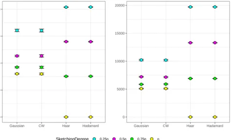
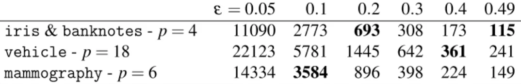
0 2000 4000 6000 8000
Gaussian CW Haar Hadamard
Frobenius Nor m n=1024, p=100 0 5000 10000 15000 20000
Gaussian CW Haar Hadamard
n=2560, p=100
SketchingDegree 0.25n 0.5n 0.75n n
Figure 2.1: Frobenius norm of the difference between the original and the sketched Gram matrix, different sketching methods (Gaussian, Clarkson-Woodruff, Haar, Hadamard), for different sketching degrees (0.25 n, 0.5n, 0.75n, 1n) and different data set sizes (1024, 2560).
2.3. MATRIX SKETCHING IN LINEAR REGRESSION 23 Figure 2.1 reports the boxplots of the Frobenius norm over the 200 replicates for the different sketching algorithms, different data sizes and four different degrees of sketching corresponding to k=n, k=0.75n k =0.5n and k =0.25n. When k =n the two orthogonal sketching methods (namely Haar and Hadamard) exactly reproduce the Gram ma-trix while, due to non-orthogonal rows, the Gaussian sketch and the Clarkson-Woodruff one give distorted results. However, especially for large datasets, when the data set size is reduced through Gaussian or Clarkson-Woodruff sketching, the approximation of the Gram matrix is better than the one obtained by the two orthogonal sketching methods. In particular, Gaussian and Clarkson-Woodruff sketching guarantee the same degree of approximation in terms of Frobenius norm but with a stronger reduction in the data set size. For this reason and for its rele-vant statistical properties, most of the following results will be referred to as Gaussian sketching.
2.3
Matrix Sketching in linear regression
Maybe the first context in which matrix sketching has been applied is multiple linear regression modeling. As previously said, the goal was to reduce the computational load related to the Gram matrix.We assume that the data consists ofn observations on a response vari-abley(which are collected in an-length vector) and a set ofpcovariates which, for the same n units, are collected in then×p matrixX. X is assumed to be of full rank. The modely=Xβ+ε is assumed to hold for the data and the goal is to find the least squares estimate for β i.e. the vectorbthat minimizes the following function:
min
b kXb−yk
2
It is well known that the solution to this problem is given by b= (X>X)−1X>y
The solution only depends on the Gram matrixX>Xand on the marginal associationX>y.
In order to review the theory related to the use of sketching methods in regression, the following quantities are worth introducing.
LetT SS=y>y;RSS=kXb−yk2
24 CHAPTER 2. MATRIX SKETCHING where T SS, RSS and MSS are the total, residual and model sum of squares respectively andR2is the multiple linear correlation coefficient. Sarl´os (2006) and Woodruff (2014), using the concept ofε-subspace embedding, proved that the linear regression problem can be rephrased in terms of sketched matrices:
min
b kSXb−Syk
2⇒min
b kXeb−eyk
2
and the solution is:
bs= (Xe>Xe)−1Xe>ey
whereSis the Sketching matrix andX˜ and ˜yare the sketched covariate matrix and response vector respectively.
bsis the so calledcomplete sketchingestimator for the vector of linear
regression coefficients.
Many theoretical results aimed at studying the properties of the sketched vector of regression coefficients provided worst case bounds.
As a consequence of theε-subspace embedding properties, Sarl´os (2006) proved that:
kbs−bk22≤ ε2 σmin2 (X)
RSS (2.1)
whereσmin2 (X)is the smallest singular value ofXandRSSis the resid-ual sum of squares of the unsketched model.
The properties of the sketched vector of regression coefficients have re-cently been studied according to a statistical perspective.
Ahfock et al. (2017) present interesting theoretical results related to the goodness of the approximation of the sketched vector with respect to the one referred to the unsketched dataset, while Dobriban & Liu (2018) mainly address the issue of the quality ofbs with respect to the
unknown vector of the model coefficientsβ.
Assuming thatyandXare fixed, Ahfocket al. studied the distribution ofbsinduced by the randomness in the sketching matrixSfor Gaussian,
Hadamard and Clarkson Woodroff sketching.
When Gaussian sketching is used it can be easily proved that, condi-tioning on the observed data set, the sketched data set has a multivariate normal distribution. In fact, each sketched observation is obtained as a linear combination of Guassian random variables.
Starting form this simple result, Ahfocket al.(2017) proved the follow-ing theorem:
2.3. MATRIX SKETCHING IN LINEAR REGRESSION 25 Theorem 2. Supposebs is computed using a Gaussian sketch and k>
p+1. The conditional distribution ofbs is:
bs|X˜,X,y∼N(b,
RSS k (X˜
>˜
X)−1)
The marginal distribution ofbsis:
bs|X,y∼Student b, RSS k−(p+1)(X >X)−1,k−(p+1) .
This means that the structured vector of regression coefficients bs
is an unbiased estimator for the vector of regression coefficientsb, ob-tained on the original dataset.
The theorem also allows to derive exact confidence intervals for the el-ements ofbs.
Things are not so straightforward for the Hadamard and Clarkson -Woodruff sketches, as they are discrete distributions over an enormous combinatorial space. The explicit finite sample distribution of the sketched estimators can be written as a sum over all these possible combinations, but such a representation is not very informative. Instead, it is use-ful to study the large n distribution of the estimator bs to obtain an
interpretable expression. An important result in Ahfock et al. (2017) is a conditional central limit theorem for the sketched dataset that con-nects the Hadamard and Clarkson-Woodruff projections to the Gaussian sketch.
Besides analyzing the quality of the regression coefficients estimated on the sketched data set with respect to the regression coefficients obtained on the full unsketched data set, Ahfocket al. also address strict inferen-tial issues. While in what has been described so far the source dataset is assumed as fixed and error is introduced by the random projection only, in the classical inferential setting a source of variability at the popula-tion level is added to the projecpopula-tion one. The properties of the sketched regression coefficients need therefore to be studied considering expec-tations both with respect to the random sketching matrices Sand with respect to sampling.
In this new setting Ahfocket al. proved that the vector of sketched re-gression coefficientsbs is an unbiased estimator for the population one
26 CHAPTER 2. MATRIX SKETCHING β and its unconditional variance after Gaussian sketching is: 1
n−p
k−p−1+1
σ2(X>X)−1
In the same inferential framework Dobriban & Liu (2018) compared the statistical efficiency of the least squares estimatorband of the sketched estimator bs for the model parameter β. In particular they considered
variance efficiency:
V E(bs,b) =
E[kbs−βk2]
E[kb−βk2] (2.2)
and prediction efficiency:
PE(bs,b) =
E[kXbs−Xβk2]
E[kXb−Xβk2]
which can be both regarded as a usual ratio of mean squared error of two estimators.
ForV Ethe parameter isβ while for PE it is the regression functionXβ. Both measures of efficiency are greater than or equal to 1, and smaller is better.
Finally they studied out-of-sample efficiency defined as:
OE(bs,b) =
E[(xt>bs−yt)2] E[(x>b−yt)2]
They considered an asymptotic framework in which both the number of variables pand the sample sizentend to infinity, and their aspect ratio converges to a constant. The size kof the sketched data is also propor-tional ton. Under these asymptotics they found the limits of the relative efficiencies under various conditions onXandS.
In particular, relying on results from asymptotic random matrix theory and free probability theory, they found very simple expressions for the
1The variance is obtained using the law of the total variance. Our result is slightly
different from Ahfocket al.’s one as they assumevarε{Es(bs|y,X)}=0 while we
think it is equal toσ2(X>X)−1asEs(bs|y,X)isb, i.e the original least squares
esti-mator.
2.3. MATRIX SKETCHING IN LINEAR REGRESSION 27 relative efficiencies in the context of iid sketching (of which the Guas-sian sketching is a special case) and of Haar/Hadamard (i.e. orthogonal sketching). They also considered uniform sampling and leverage based sampling, but we will report here on the sketching methods only. Both for Gaussian sketching and Haar/Hadamard sketching the limits of the variance efficiency and of the prediction efficiency coincide and are respectively:
1+ n−p
k−p−1 for Gaussian sketch 2
n−p
k−p for Haar/Hadamard sketch
It can be easily noticed that the estimation error increases by the fac-tor due to sketching and that it increases for Haar and Hadamard sketch less than for the iid sketch.
This is partially coherent with our finding in the previous section (which however involves the Gram matrix only and does not consider the effect of sketching on the association between the response and the covari-ates). Gaussian projections distort the geometry of Euclidean space due to their non-orthogonality and this in turn degrades the performance of OLS even if we do not reduce the sample size.
The difference between the efficiency of the different sketching meth-ods decreases as the size of the sketched data sets decreases.
The limits for OE are nnk−p(k−p2) and nk((n−pk−p)) respectively for the Gaussian and the orthogonal sketching.
In the same paper, in which they studied how the regression coeffi-cients obtained after sketching both X andy approximate the ones re-ferred to the unsketched dataset, Ahfocket al.(2017) also studied what they calledpartial sketching, which has been introduced in the litera-ture by Dhillonet al.(2013) and Pilanci & Wainwright (2016).
As the computational burden mainly affects the Gram Matrix, one can simply sketch the design matrix Xwhile leaving the response variable yunchanged. The least squares problem can be rephrased as
min
b kSX b−yk
2⇒min
b kX be −yk
2
28 CHAPTER 2. MATRIX SKETCHING and the solution is the so-called vector of partially sketched regression coefficients:
bp = (Xe>X)e −1X>y
Ahfocket al.proved that:
kbp−bk2≤
4ε2 σmin2 (X)
MSS (2.3)
i.e. the goodness of the approximation of the partially sketched regres-sion coefficients with respect to the ones obtained on the full data set is upper bounded by a quantity that depends on the unsketched model sum of squaresMSS. This means that when the model sum of squares is low partial sketching provides a better approximation than complete sketching; on the contrary when the error sum of squares is low com-plete sketching should be preferred.
When dealing with Gaussian sketching, the following results hold:
e
X|X∼MN(0k×p,Ik,1
kX
>X)
(2.4) i.e. ˜Xis a matrix variate normal random variable. Therefore:
e
X>Xe|X∼Wishart(k,X>X/k) (2.5)
and (Xe>X)e −1|X∼InvWishart(k,k(X>X)−1) (2.6)
Useful properties of the Wishart and the inverse-Wishart random vari-ables are reported in Appendix A. We will refer to them in the following. bp= (Xe>X)e −1X>yis therefore a linear combination of the elements of
an inverse Wishart random variable.
Its distribution is unknown but it is possible to compute its expected value and its variance.
According to propertyA6(i)in the appendix:
E h (Xe>X)e −1 i = 1 k−p−1(X >X)−1. From this: Es[bp|y,X] =E h (Xe>X)e −1X>y|y,X i = k (k−p−1)b (2.7)
2.3. MATRIX SKETCHING IN LINEAR REGRESSION 29 easily derives. The subscripts stresses the fact that the expected value is computed with respect to all possible sketching matrices.
This result means that the partially sketched vector of regression coeffi-cientsbpis a biased estimator of the corresponding vectorbreferred to
the full data set.
The unbiased estimator can therefore be obtained as: b∗p =(k−p−1)
k (Xe
>
e
X)−1X>y.
Ahfock et al. also derived the variance both for the biased and the unbiased vector of partially sketched regression coefficients:
V(bp) = k2 (k−p)(k−p−1)(k−p−3)(MSS(X >X)−1+k−p+1 k−p−1bb >) (2.8) V(b∗p) = (k−p−1) (k−p)(k−p−3)(MSS(X >X)−1+k−p+1 k−p−1bb >) (2.9)
Their proof is a little bit laborious. We have obtained the same result in a simpler way by relying on the result in Haff (1979) which is reported inA6(iii)in the appendix.
As: V(bp) =E(bp2)−E(bp)2 and, according to (2.7): E(bp)2= k2 (k−p−1)2bb >
we only need to find a suitable expression forE(bp2)in order to obtain
the result.
E(bp2) =E(bpbp>) =E
h
(Xe>X)e −1X>yy>X(Xe>X)e −1 i
which, after setting X>yy>X=A and using the property in A6(iii), becomes: E h (Xe>X)e −1A(Xe>X)e −1 i = 1 (k−p)(k−p−1)(k−p−3)tr(k(X >X)−1A)k(X>X)−1+ + 1 (k−p)(k−p−3)k(X > X)−1A(X>X)−1k
30 CHAPTER 2. MATRIX SKETCHING But: (X>X)−1A(X>X)−1= (X>X)−1X>yy>X(X>X)−1=bb> Moreover: tr[k(X>X)−1A)](X>X)−1=k2tr[(X>X)−1X>yy>X](X>X)−1 =k2tr[by>X](X>X)−1
and, after applying trace properties and recognizing inb>X>y the model sum of squares for the full data set, it becomes:
k2tr[b>X>y](X>X)−1=k2MSS(X>X)−1 So: E(bp2) = k2 (k−p)(k−p−1)(k−p−3)MSS(X >X)−1+ k2 (k−p)(k−p−3)bb >
The variance then becomes:
V(bp) = k2 (k−p)(k−p−1)(k−p−3)MSS(X >X)−1+ + k 2 (k−p)(k−p−3)bb >− k2 (k−p−1)2bb > = k 2 (k−p)(k−p−1)(k−p−3)(MSS(X >X)−1+k−p+1 k−p−1bb >)
The variance ofb∗p can be derived accordingly.
It is immediately evident that the variance of the partially sketched re-gression coefficients depends on the model sum of squares while the one of the completely sketched regression coefficients depends on the residual sum of squares. This means that whenR2is close to 1 complete sketching can be more efficient than partial sketching while whenR2is close to zero the latter should be preferred.
In order to deal with intermediate situations, Ahfocket al. (2017) pro-pose a combined estimator which relies on the incorrelation betweenb∗p andbs.
As previously said, the explicit form of the sampling distribution of the partially sketched regression coefficients is hard to obtain. However, by
2.3. MATRIX SKETCHING IN LINEAR REGRESSION 31 making a connection with method of moments estimation, Ahfock et al. also established asymptotic normality of bothbp andb∗p ask tends
to infinity. This motivates the construction of approximate confidence intervals.
They also proved that, asymptotically, the Hadamard and Clarkson-Woodruff sketches should have similar mean and variance properties to the Gaussian partially sketched estimator.
Dobriban & Liu (2018) did not address the issue related to the effi-ciency of partial sketching in the unconditional setting, but Ahfock et al. proved thatb∗p is also unbiased for the population parameterβ, and its variance is:
Vε(b∗p) = (k−p−1) (k−p)(k−p−3){(pσ 2+n τ2)(X>X)−1+ + (k−p+1 k−p−1σ 2(X>X)−1+k−p+1 k−p−1β β >)}
whereσ2is the variance of the error term andτ2=kXβk22/nrepresents the average mean function sum of squares.
When compared with the unconditional variance of bs, this variance
tells us that againbs is more efficient when the signal to noise ratio is
high andb∗p is more efficient when the signal to noise ratio is low. This is confirmed also when variance efficiency ofb∗pin estimatingβ in (2.2) is measured with respect to the ordinary least squares estimator.
Chapter 3
Matrix Sketching for LDA
3.1
Introduction
The main contribution of this thesis is the proposal of applying ma-trix sketching in linear discriminant analysis. As illustrated in chapter 1 LDA can be seen as a particular regression problem, therefore the same computational load inherent in the computation of the Gram matrix in-volved in multiple linear regression also affects LDA.
As the response variable for two group LDA is a binary variable, partial sketching represents the only viable solution. Sketching the response variable too (i.e. linearly combining the response values) would lead to loose the information on group membership, thus preventing any possi-ble classification.
According to the partial sketching approach, only the Gram matrix is sketched while the relationship between the predictor variables and the response is left unchanged.
By applying matrix sketching to the Gram matrix involved in (1.9), (1.10), (1.11) and (1.12), the following expression for the partially sketched linear discriminant direction can be obtained:
bp = (Xe>X)e −1(x¯1−x¯0) n0n1 n0+n1 (3.1) ap =γpbp (3.2) 33
34 CHAPTER 3. MATRIX SKETCHING FOR LDA where: γp=(n−2) (n0+n1) n0n1 + (x¯1−x¯0) >W−1 sk (x¯1−x¯0) (3.3) =(n−2) n n0n1 1 1−n0n1 n (x¯1−x¯0)>(Xe>X)e −1(x¯1−x¯0) (3.4)
Equivalentlyap can be written as:
ap=Wsk−1(x¯1−x¯0) = (n−2) (Xe>Xe−B)−1(x¯1−x¯0) =γpbp (3.5)
3.2
Theoretical Results
In analogy with the approach followed in the context of multiple regression, we have derived an upper bound for the squared Euclidean distance between the vector of the partially sketched linear discriminant coefficients ap and the linear discriminant direction a referred to the
unsketched dataset:
Theorem 3. Suppose that Xe is an ε−subspace embedding of X, with
0<ε <0.5.Then the following bound holds:
ka−apk22≤dM2 h (n−2) +n0n1 n d 2 M i 1 σmin2 (X)4ε 2 (3.6) Proof. ka−apk2=kγb−γpbpk2 = n n0n1(n−2) k 1 1−n0n1 n δ2 b− 1 1−n0n1 n δp2 bpk22 where:δp2= (x¯1−x¯0)>(Xe>X)e −1(x¯1−x¯0)∈R and δ2= (x¯1−x¯0)>(X>X)−1(x¯1−x¯0)
LetX=UDV> be the singular value decomposition ofX. Then: b= (X>X)−1(x¯1−x¯0) n0n1 n = ((UDV>)>UDV>)−1(x¯1−x¯0) n0n1 n =VD−1D−1V>(x¯1−x¯0) n0n1 n , becauseU >U=I p
3.2. THEORETICAL RESULTS 35 Similarly,bp can be written as:
bp= (Xe>X)e −1(x¯1−x¯0) n0n1 n = ((SX)>SX)−1(x¯1−x¯0) n0n1 n =VD−1(U>S>SU)−1D−1V>(x¯1−x¯0) n0n1 n So: ka−apk2= (n−2)k 1 1−n0n1 n δ2 VD−1D−1V>(x¯1−x¯0)+ − 1 1−n0n1 n δp2 VD−1(U>S>SU)−1D−1V>(x¯1−x¯0)k2 = (n−2)kVD−1 " 1 1−n0n1 n δ2 I− 1 1−n0n1 n δp2 (U>S>SU)−1 # D−1V> (x¯1−x¯0)k2 Let: ξ = 1 1−n0n1 n δ2 ∈R, andψ= 1 1−n0n1 n δp2 ∈R, with bothψ,ξ >0 Then: ka−apk2= (n−2)kVD−1 h ξ I−ψ(U>S>SU)−1 i D−1V>(x¯1−x¯0)k2 ≤(n−2)kVD−1k2kξ I−ψ(U>S>SU)−1k2kD−1V>(x¯1−x¯0)k2 As:kVD−1k2= 1
σmin(X),whereσmin(X)is the minimum singular value ofX, and: kD−1V>(x¯1−x¯0)k22= (x¯1−x¯0)>VD−1D−1V>(x¯1−x¯0) = (x¯1−x¯0)>(X>X)−1(x¯1−x¯0) =δ2 ⇒ kD−1V>(x¯1−x¯0)k2=δ then: ka−apk2≤(n−2) 1 σmin(X) δkψ(U>S>SU)−1−ξ Ik2
36 CHAPTER 3. MATRIX SKETCHING FOR LDA We now need to upper bound the maximum singular value of the matrixψ(U>S>SU)−1−ξ I. We can write: kψ(U>S>SU)−1−ξ Ik2=ξk ψ ξ M −1− Ik2, whereM=U>S>SU. Since: ψ ξ = 1−n0n1 n δ 1−n0n1 n δp ∼1 then: kψ(U>S>SU)−1−ξ Ik2=ξkM−1−Ik2,
The maximum absolute value of the singular values of the matrixM−1−I is equal to: max 1 σmin(M) −1 , 1 σmax(M) −1 ,
whereσmin(M)andσmax(M)are the minimum and maximum singular
value ofMrespectively.
SinceSis anε−subspace embedding forX:
σmin(M)≥1−ε,σmax(M)≤1+ε
this implies that:
1 σmax(M) ≤ 1 σmin(M) ≤ 1 1−ε So: kψ(U>S>SU)−1−ξ Ik2=ξkM−1−Ik2 =ξmax( 1 σmin(M) −1, 1 σmax(M) −1) ≤ξ 1 1−ε −1 ≤ξ 2ε = 1 1−n0n1 n δ2 2ε
3.2. THEORETICAL RESULTS 37 So: ka−apk2≤(n−2) 1 σmin(X) δ 1 1−n0n1 n δ2 2ε Now, remembering that:
dM2(x¯0,x¯1) = (n−2) δ2 1−n0n1 n δ2 then: (n−2) 1 1−n0n1 n δ2 =d 2 M(x¯0,x¯1) δ2 So: ka−apk2≤ d2M(x¯0,x¯1) δ 1 σmin(X) 2ε Squaring both sides, we have:
ka−apk22≤ dM4(x¯0,x¯1) δ2 1 σmin2 (X) 4ε2 Since: δ2= (x¯1−x¯0)>(X>X)−1(x¯1−x¯0) = dM2 (n−2) +n0n1 n d 2 M
the bound can finally be rewritten as:
ka−apk22≤dM2 h (n−2) +n0n1 n d 2 M i 1 σmin2 (X) 4ε2
The bound essentially depends on the squared Mahalanobis distance (like bp that depends on MSS) as the effect of n is compensated by
σmin(X) according to the so called interlacing theorem which, when
referred to singular values, states what follows:
Theorem 4. For A ∈ Cn×p, let B denote A with one of its rows or columns deleted. Then:
σi+1(A)≤σi(B)≤σi(A)
where σiis the i-th singular value in the decreasing sequence of the p
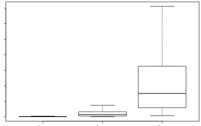
38 CHAPTER 3. MATRIX SKETCHING FOR LDA This implies that, as the number of rows increases, the minimum singular value does too (see for further details Horn & Johnson, 1991). To better understand the meaning of the bound, we have performed a small simulation study in which we have generated 100 samples com-posed of n0=n1 =10000 units from p-variate Normal distributions, with p = 4 and squared Mahalanobis distance equal to 5.6,11.5,23 (these values are very close to the ones of the empirical data sets de-scribed in 3.3). The data have then been sketched to k=1000. Fig-ure 3.1 reports the boxplot of the euclidean distances between the par-tially sketched and the unsketched linear discriminant directions over the replicates. The results confirm that that the median distance and the variability increase as the Mahalanobis distance increases and the upper extreme of the boxplot is within the bound in (3.6).
This result is meaningful also from a statistical perspective. When the populations are separated, a plurality of different discriminant direc-tions separates the two groups equally well, while less variability is allowed when the populations are increasingly overlapping.
dM 2 =5.6 dM 2 =11.5 dM 2 =23 0 5 10 15 20 25 30 35 ||ap−a|| 2 − Homoscedastic populations
Figure 3.1: Boxplot of the euclidean distances between the partially sketched and the unsketched linear discriminant directions over 100 replicates, from multivariate normal distributions with varying Maha-lanobis distance.
3.2. THEORETICAL RESULTS 39
Besides deriving the approximation bound according to a numeric analytic perspective we have also studied the properties of the sketched discriminant direction within an inferential framework. Our goal would be first of all to derive the expected value and the variance of the sketched linear discriminant direction, in analogy to the approach followed for linear regression.
Proposition 3.1. The random variableap (where randomness is due to
S) has finite expected value.
Proof. According to (2.4), (2.5), (2.6): e X|y,X∼MN(0k×p,Ik, 1 kX >X) Therefore: e X>Xe|y,X∼Wishart(k,X>X/k) (Xe>X)e −1|y,X∼InvWishart(k,k(X>X)−1) According to (3.3) and (3.4): ap =γpbp = (n−2) n n0n1 1 1−n0n1 n (x¯1−x¯0)>(Xe>X)e −1(x¯1−x¯0) (Xe>X)e −1(x¯1−x¯0) n0n1 n = (n−2) 1 1−n0n1 n (x¯1−x¯0)>(Xe>X)e −1(x¯1−x¯0) (Xe>X)e −1(x¯1−x¯0) Settingu= (x¯1−x¯0),G=Xe>Xe,Λ=X>X u>ap= (n−2) 1 1−n0n1 n u>G−1u u>G−1u = (n−2) 1−n0n1 n u>G−1u u>Λ−1u u >Λ−1u u>G−1u u>Λ−1u u > Λ−1u where: u >G−1u u>Λ−1u = 1 z ∼ 1 χn−2 p−1
40 CHAPTER 3. MATRIX SKETCHING FOR LDA This result is a consequence of property A4:
E h u>ap i = (n−2)E " 1 1−n0n1 n 1 zu>Λ−1u 1 z u > Λ−1u # = (n−2)E 1 z−n0n1 n u>Λ−1u u>Λ−1u =ω Z +∞ 0 1 z−n0n1 n u > Λ−1u | {z } u>Λ−1uz( n−p−1 2 −1)e− z 2 dz δ where ω = (n−2) 2n−2p−1 Γ(n−p−1 2 ) The singularity point n0n1
n δ can be taken out asCauchy principal value
transformation, resulting in a finite expected value ofu>ap:
=ω lim ε→0+ " Z n0n1 n δ−ε 0 1 z−n0n1 n δ u>Λ−1uz( n−p−1 2 −1)e− z 2 dz+ Z +∞ n0n1 n δ+ε 1 z−n0n1 n δ u>Λ−1uz(n−2p−1−1)e− z 2 dz <∞
Technical details of the proof are omitted.
This result tells us that a finite linear combination of ap has finite
ex-pected value. This in turn allows to say that the variable ap has finite
expected value, but it doesn’t give any hint on how to compute it. The distribution of ap is a function of the inverse of a shifted Wishart and
its moments are not known. In order to study the properties of ap, we
derive an approximation for its expected value through its series expan-sion.
Proposition 3.2. A first-order approximation of the expected value of
ap is given by: Es(ap) = (n−2)E (Xe>Xe−B)−1 (x¯1−x¯0) (3.7) =η+ (α−η) (n−2)nn 0n1 (n−2)nn 0n1+d 2 M(x¯0,x¯1) a (3.8)
3.2. THEORETICAL RESULTS 41
where: α = k−p−k 1 andη= k
2
(k−p)(k−p−3)
Proof. Recalling that Taylor’s expansion of the inverse of the sum of
two matrices is:
(A+B)−1=A−1−A−1BA−1+A−1BA−1BA−1+
−A−1BA−1BA−1BA−1+· · ·
whereAandA+Bare invertible andkA−1Bk<1 orkBA−1k<1, we derive Taylor’s expansion of(Xe>Xe−B)−1and we truncate it to the first
order, as higher order terms involve quadratic forms of quadratic forms of inverted Wishart random variables whose moments have not a closed form expression (for the same reason no closed form for the variance of ap can be derived either).
E h (Xe>Xe−B)−1 i =E h (Xe>X)e −1 i +E h (Xe>X)e −1B(Xe>X)e −1 i Furthermore, according to (1.13): (X>X−B)−1= (X>X)−1+ 1 1−g(X >X)−1 B(X>X)−1 where:g=tr(X>X)−1B=n0n1 n (x¯1−x¯0)>(X>X)−1(x¯1−x¯0) = n0n1 n δ2
The two expressions coincide wheng=0.
In empirical applications of LDAgis always very close to 0, so assum-ing it equals 0 does not cause a too relevant loss.
42 CHAPTER 3. MATRIX SKETCHING FOR LDA Using the results in Haff (1979) reported in A6 (i) (iii) we have:
E h (Xe>Xe−B)−1 i =E h (Xe>X)e −1 i +E h (Xe>X)e −1B(Xe>X)e −1 i = k (k−p−1)(X >X)−1+ tr(−k(X>X)−1B) (k−p)(k−p−1)(k−p−3)· ·k(X>X)−1+ 1 (k−p)(k−p−3)k(X >X)−1B(X>X)−1k = k (k−p−1)(X >X)−1− k2g (k−p)(k−p−1)(k−p−3)· ·(X>X)−1+ k 2 (k−p)(k−p−3)(X >X)−1B(X>X)−1 = k (k−p−1)(X >X)−1+ k2 (k−p)(k−p−3)(X >X)−1B(X>X)−1 =α (X>X)−1+η (X>X)−1B(X>X)−1 where we setα = k (k−p−1) andη= k2 (k−p)(k−p−3) So, using (3.5): E(ap) = (n−2)E(Xe>Xe−B)−1 (x¯1−x¯0) = (n−2) h α (X>X)−1+η (X>X)−1B(X>X)−1 i (x¯1−x¯0) = (n−2)hη (X>X)−1+ (X>X)−1B(X>X)−1+ (α−η)(X>X)−1i(x¯1−x¯0) = (n−2)η (X>X)−1+ (X>X)−1B(X>X)−1(x¯1−x¯0)+ + (n−2) (α−η)(X>X)−1(x¯1−x¯0) = (n−2)η(X>X−B)−1(x¯1−x¯0) + (n−2) (α−η)(X>X)−1(x¯1−x¯0) =ηW−1(x¯1−x¯0) + (n−2) (α−η)(X>X)−1(x¯1−x¯0) =ηa+ (n−2) (α−η)(X>X)−1(x¯1−x¯0) Now, rembering that, for (1.10) and (1.11): a=γ b=γ(X>X)−1(x¯1−x¯0) n0n1 n , whereγ = n n0n1(n−2) +d 2 M(x¯0,x¯1) we obtain:(X>X)−1(x¯1−x¯0) =1 γ n n0n1 a= n n0n1 n n0n1(n−2) +d 2 M(x¯0,x¯1) a
3.3. REAL DATA APPLICATIONS 43 So: Es(ap) =η a+ (n−2) (α−η) n n0n1 n n0n1(n−2) +d 2 M(x¯0,x¯1) a = " η + (α−η) n n0n1(n−2) n n0n1(n−2) +d 2 M(x¯0,x¯1) # a
This result tells us thatapis a biased estimator ofaand that the bias
depends again on the Mahalanobis distance between the two groups in the full dataset. De-biasing ap would involve computing the
Maha-lanobis distance in the original data set, thus making the use of sketch-ing meansketch-ingless. For this reason in the applications that follow we will not make any correction toap.
It is worth noting that while (X>X−B)−1 is positive definite by definition, nothing guarantees that (X˜>X˜ −B)−1 is also positive defi-nite because sketching the Gram matrix only (i.e. using partial sketch-ing) breaks the link between the sketched total sum of squares and the unsketched between group sum of squares. In empirical applications a check should be made on the positive definiteness of(X˜>X˜ −B)−1and solutions that deviate from it should be discarded.
3.3
Real data applications
The goal of supervised classification is to definite an assignment rule that has the best accuracy. We expect that sketching can cause a loss in terms of accuracy with respect to the rule obtained on the full data set. In order to better understand how sketching impacts on the accuracy of LDA we have analyzed several real data sets with different degrees of sketching and different sketching methods.
Each data set has been randomly split in two parts: 75% of the units for both classes constituted the training set and the remaining 25% formed the test set. The procedure was repeated 200 times. The values in the table represent the median of the quantity of interest over the 200 repli-cates.
44 CHAPTER 3. MATRIX SKETCHING FOR LDA also small data set, which in principle would not require sketching, in order to have a more detailed picture of how sketching works.
Here we present the results on four of them which are briefly described in the following.
• iris: the famous (Fisher’s or Anderson’s) iris data set gives the
mea-surements in centimeters of the variables sepal length and width and petal length and width, respectively, for 50 flowers from each of 3 species of iris. Here the samples are labeled as virginica vs. nonvir-ginica.
• vehicle: data include the silhouettes measured by the HIPS (Hi-erarchical Image Processing System) of 846 vehicles, extracted in
18 features. The aim is to distinguish the vans from the other
ve-hicles. (https://archive.ics.uci.edu/ml/datasets/Statlog+
(Vehicle+Silhouettes)).
• banknotes: data extracted from 1372 images of genuine and forged banknote-like specimens. Wavelet Transform tool were used to extract
4 features from images. (http://archive.ics.uci.edu/ml).
• mammography: the Mammography dataset (Woodset al., 1993) has 6 attributes and 11,183 samples that are labeled as noncalcification and calcifications.
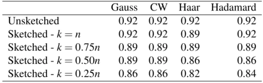
Table 3.1: iris dataset, n=150 - Accuracy median values (over 200 replications)
Gauss CW Haar Hadamard
Unsketched 0.92 0.92 0.92 0.92
Sketched -k=n 0.92 0.92 0.89 0.92
Sketched -k=0.75n 0.89 0.89 0.89 0.89
Sketched -k=0.50n 0.89 0.89 0.86 0.86
3.3. REAL DATA APPLICATIONS 45 Table 3.2: vehicles dataset, n=846 - Accuracy median values (over 200 replications)
Gauss CW Haar Hadamard
Unsketched 0.95 0.95 0.95 0.95
Sketched -k=n 0.95 0.95 0.95 0.95
Sketched -k=0.75n 0.95 0.95 0.95 0.95
Sketched -k=0.50n 0.94 0.94 0.93 0.93
Sketched -k=0.25n 0.93 0.93 0.89 0.89
Table 3.3: banknotes data, n=1372 - Accuracy median values (over 200 replications)
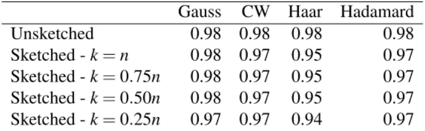
Gauss CW Haar Hadamard
Unsketched 0.98 0.98 0.98 0.98
Sketched -k=n 0.98 0.97 0.95 0.97
Sketched -k=0.75n 0.98 0.97 0.95 0.97
Sketched -k=0.50n 0.98 0.97 0.95 0.97
Sketched -k=0.25n 0.97 0.97 0.94 0.97
Table 3.4: mammography data, n=11,183 - Accuracy median values (over 200 replications)
Gauss CW Haar Hadamard
Unsketched 0.98 0.98 0.98 0.98
Sketched -k=n 0.98 0.98 0.98 0.98
Sketched -k=0.75n 0.98 0.98 0.97 0.97
Sketched -k=0.50n 0.98 0.98 0.97 0.96
Sketched -k=0.25n 0.98 0.98 0.97 0.95
All the empirical results show that sketching has a very little im-pact on accuracy, which remains almost unchanged in all the cases, even when, for k=0.25n, the data set size is reduced to one fourth. Gaussian and Clarkson-Woodruff sketches seem to guarantee the best
46 CHAPTER 3. MATRIX SKETCHING FOR LDA performances.
The only case in which the performances are really deteriorated is for the Iris data (see Table 3.1). However table 3.5 shows that the number of available units in that case is below the limit required by Johnson and Lindenstrauss Lemma even for a precision corresponding to ε =0.49 which yields the worst possible approximation. In all the other cases the accuracies are preserved even for sketching degrees that do not al-low to guarantee a good approximation of the discriminant direction. The table shows the value ofkrequired by Johnson Lindenstrauss Lemma for the different number of variables in the different datasets that have been analyzed and for different quality of approximation correspond-ing to different values of ε. The larger the value of ε the worse the approximation.
Table 3.5: Minimum value of k= 20 logp
ε2 required to obtain a given approximation ofεfor the different number of variables in the empirical data sets. In bold the values ofkcompatible with the observed number of units (ntraining =112 for iris, ntraining=634 forvehicle, ntraining = 1029 forbanknotes,ntraining=8387mammography).
ε =0.05 0.1 0.2 0.3 0.4 0.49
iris&banknotes-p=4 11090 2773 693 308 173 115
vehicle- p=18 22123 5781 1445 642 361 241
Chapter 4
Matrix Sketching for
imbalanced classes
4.1
Introduction
In many practical contexts, observations have to be classified into two classes of remarkably distinct size.
In such cases, many established classifiers often trivially classify in-stances into the majority class achieving an optimal overall misclassifi-cation error rate.
This leads to poor performance in classifying the minority class, the correct identification of which is usually of more practical interest. The presence of imbalanced classes in the big data context also poses relevant computational issues. If the dataset contains thousands or mil-lions of observations from the majority class for each example from the minority one, many of the majority class observations are redundant. Their presence increases the computational cost with no advantage in terms of classification accuracy.
The problem of imbalanced classes is very common in modern clas-sification problems and has received a great attention in the machine learning literature (Chawlaet al., 2004).
The error rate, or its complement, accuracy, is the most widely used measure of classifier performance. However, it inevitably favors the majority class when the misclassification error has the same importance for the two classes. On the contrary, when the error in the minority class is more important than the one of the majority class, the receiver
48CHAPTER 4. MATRIX SKETCHING FOR IMBALANCED CLASSES ing characteristic (ROC) curve and the area under the curve (AUC) are commonly suggested.
The ROC curve is a plot of the true positive rate (sensitivity) versus the false positive rate (1−specificity) and hence a higher AUC generally in-dicates a better classifier.
The ROC is obtained by varying the discriminant threshold, while the error rate is obtained at an optimal discriminant threshold. Therefore, AUC is independent of the discriminant threshold, while the accuracy is not.
The literature on the problem of supervised classification is very broad and methodological solutions follow two main streams. People either suggest to modify the loss function used in the construction of the clas-sification rule or propose to re-balance the data.
The first solution requires, in most of the cases, the definition of a loss function that is specific for the case at hand and therefore not easily gen-eralizable to different empirical problems. Re-balancing strategies are more general and not problem specific. That explains their great suc-cess in applied research and the focus on explaining their performances and on improving them.
Re-balancing the class sizes in the training dataset, is usually obtained either by oversampling the minority class or by under-sampling the ma-jority class, or by a combination of both. The rebalanced data are then used to train the classifiers.
As far as two-class linear discriminant analysis is concerned, the prob-lem has been addressed, among others, by Xie & Qiu (2007), Xue & Titterington (2008), Xue & Hall (2014).
Through a wide simulation study supported by theoretical considera-tions, Xue & Titterington (2008) showed that AUC generally favors balanced data but the increase in the median AUC for LDA after re-balancing is relatively small. On the contrary, error rate favors the orig-inal data and re-balancing causes a sharp increase in the median error rate. They also stress that re-balancing affects the performances of LDA in both the equal and unequal covariance case.
Xue & Hall (2014) proved that, in the Gaussian case, using the rebal-anced training data can often increase the area under the ROC curve (AUC) for the original, imbalanced test data. In particular they demon-strate that, at least for LDA, there is an intrinsic, positive relationship between the re-balancing of class sizes and the improvement of AUC
4.1. INTRODUCTION 49 and the largest improvement in AUC can be achieved, asymptotically, when the two classes are fully rebalanced to be of equal sizes.
AUCmax=Φ
q
(x¯1−x¯0)>(S1+S0)−1(x¯1−x¯0)
where, now and henceforth, the subscript 1 identifies the minority class. However, when the two Gaussian classes have similar covariance matri-ces, re-balancing class sizes only provides a little improvement in AUC for LDA.
Moreover, re-balancing class sizes may not improve AUC when LDA is applied to non-Gaussian data.
In both the above mentioned papers re-balancing is obtained either by randomly undersampling the largest class or by randomly oversampling the smallest one.
It has however been argued that random undersampling may lose some relevant information while randomly oversampling with replacement the smallest c