Machine-learning-based vehicle delay prediction at signalized intersections

(1)

(2)

MACHINE-LEARNING-BASED VEHICLE DELAY PREDICTION AT SIGNALIZED INTERSECTIONS

BY

BEHNOUSH GARSHASEBI

THESIS

Submitted in partial fulfillment of the requirements for the degree of Master of Science in Civil Engineering

in the Graduate College of the

University of Illinois at Urbana-Champaign, 2018

Urbana, Illinois Adviser:

(3)

ABSTRACT

Delay is one of the critical elements of signalized intersections performance measures. Field delay calculations are usually time-consuming and inefficient and dominantly rely on manual observations and post-calculations or complicated infrastructure configurations of detectors and vehicular sensors; making quick and reliable decision making difficult for practitioners. In this thesis, we implement the machine learning methods such as Linear Regression (LR), Support Vector Regression (SVR), and Random Forest (RF) to construct fast and straightforward models for vehicle delay prediction at signalized intersections. The models are trained by the use of available data sources such as signal timing plan and queue length per cycle. A thorough comparison between the performance of different machine learning models is also provided. To the best of our knowledge, this is the first study that implements machine-learning approaches to develop prediction models for vehicle delay at signalized intersections. Our study area consists of five signalized intersections along the Neil Street corridor (Major Street), Champaign, IL. Four of the crossing streets create typical four-legged intersections, and one of them create three-legged intersection; including one Major Street and five Minor Streets. We have observed that among the three models, LR and RF models achieved the best performances in predicting vehicle delay per cycle on the major streets when cycle length, green time and queue length are used as the predictors. LR predictions for the vehicle delay per cycle on the major street had an average error of 5.3 seconds, compared to the field vehicle delay per cycle and the R-squared of the LR model is 0.62; which shows that the model is able to explain 62% of the variation in the vehicle delay on the major street. Also, for the LR, the average accuracy (1-MRE) was 55%, 63% and 51% for the combined dataset, major street dataset, and minor streets dataset, respectively. On the other hand, RF predictions for the vehicle delay per cycle on the major street had an average error of 5.2 seconds, compared to the field vehicle delay per cycle. For the RF, the average accuracy (1-MRE) was 61%, 65% and 55% for the combined dataset, major street dataset, and minor streets dataset, respectively. Furthermore, on the major street, LR had errors less than 6 seconds in 87% of the predictions; and RF had errors less than 6 seconds in 80% of the predictions. This study shows that the effectiveness of the LR model for vehicle delay prediction on the major street is promising and manifested. Therefore, the straightforward LR predictive model proposed in this study, can be applied as an efficient tool to understand the current level of service at signalized intersections

(4)

quickly. Rapid performance assessment further identifies the problems of the signal timing plan and enables the practitioners to make decisions on necessary remedial actions.

Keyword: signalized intersections, vehicle delay, machine learning, prediction models, data-driven models, delay prediction

(5)

(6)

ACKNOWLEDGEMENTS

First and foremost, I would like to express my sincere appreciation and thanks to my advisor Professor Rahim. F. Benekohal for giving me the opportunity to be a part of his research group and all the assistance and support he has provided me along the way. I am inspired by his dedication and commitment to the profession and his patience in training the students. I feel I have learned a lot during my time working at Professor Benekohal’s research group and I consider myself extremely lucky to have such advisor; and I am deeply indebted for all his encouragements and his trust in my abilities.

I would also like to acknowledge that the data for this study is provided by the dataset in the ICT-R27-127; the project of the Safety and Efficiency Benefits of Implementing Adaptive Signal Control Technology in Illinois. ICT-R27-127 was conducted in cooperation with the Illinois Center for Transportation; the Illinois Department of Transportation; and the U.S. Department of Transportation, Federal Highway Administration.

(7)

CHAPTER 1: INTRODUCTION

Measuring the performance of traffic at signalized intersections is one of the most essential tasks in determining the level of service at signalized intersections. Delay calculation is one of the critical elements of the signalized intersections performance analysis. Currently there are several methods to measure the performance of signalized intersections, but their capabilities in dynamically estimating vehicle delay are limited. Field delay calculations are usually time-consuming and complicated. Over the past decade, real-time traffic data at signalized intersections is recorded and made available to the traffic signal operators. Using these traffic data, researchers have been able to develop delay estimation models. However, previous studies have not been focusing on using statistical and machine learning models to predict vehicle delay at signalized intersections. This study presents a systematic and comprehensive framework for constructing machine-learning-based predictive models for predicting vehicle delay per cycle at signalized intersections. We consider three different machine-learning models, namely the Linear Regression (LR), the Support Vector Regression (SVR), and The Random Forest (RF) Regression. We will present a thorough comparison between the performance of these three models in delay prediction.

The majority of the methods that are commonly used rely excessively on detectors and sensors equipment for data collection. In this study, we aim at using the least amount of available data sources to predict the delay at signalized intersections; data sources like, the signal timing plan and field queue length data counts; which are easily collected in the field by a relatively simple procedure presented in the Highway Capacity Manual (HCM 2016). For developing the prediction models in this study, we first performed an extensive data collection by using recorded videos at five intersections along a corridor in Champaign, IL and conducted a data reduction for a cycle-by-cycle field data preparation. Field data like vehicle delay, queue length, signal timing plan, volume, etc. were collected. Next, the prepared dataset is utilized as the training data for our predictive models.

Also, calculating the vehicle delay using the method presented in the Highway Capacity Manual (HCM 2016), which is a frequently used, is a time-consuming process that requires

(9)

automate delay data collection or estimation to obtain accurate and reliable information within minutes instead of hours or days. Although several dynamic methods have been developed to estimate vehicle delay, all of the models need extensive data collection.

Hence, there is a need for a new dynamic delay calculation method that uses least amount of data sources and can be implemented efficiently through the current signal systems configurations at signalized intersections. This study fulfills the need for developing a new vehicle delay prediction method that can be implemented at signalized intersections without depending on the detector’s infrastructure.

1.1 OBJECTIVE

The objective of this research is to develop a model to predict vehicle delay per cycle, using existing field traffic data sources, like signal timing plan and easily-collected queue length data. The purpose of this study is to predict the delay for through lane vehicles. While most automated vehicle delay prediction studies in the past have focused on inventing new technologies to estimate traffic delay using detectors infrastructure and traffic data collection configurations, this study has focused on development of a methodology that can be applied to the existing data sources which is mostly available by the traffic signal operators or easily collected in the field.

1.2 SCOPE

This research first presents vehicle delay prediction models which are trained by the use of real-world field vehicle delay per cycle data. The original dataset contains a major street and five minor streets combined data, although the different models are trained for a combined dataset of major and minor streets, a major street dataset individually, and a minor streets dataset individually. Then, this research evaluates and compares the models and suggests the most efficient model for the corresponding dataset.

1.3 THESIS ORGANIZATION

This thesis is organized into six chapters. Chapter 1 includes an introduction, and the objective and scope of the study. Chapter 2 presents a literature review of the available research relating to the topic of vehicle delay estimation. This chapter summarizes different research studies that have shown some success in modeling the delay estimation. Chapter 3 presents a problem

(10)

description. Chapter 4 presents the predictive models training and their prediction results. Chapter 5 provides a discussion on the results. Finally, Chapter 6 presents a conclusion and also recommendations for future studies.

(11)

CHAPTER 2: STATE OF THE PRACTICE IN DELAY PREDICTION

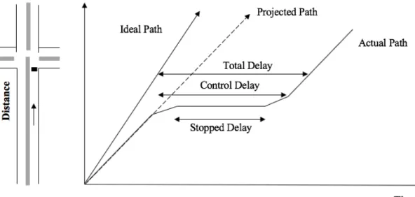
Vehicle delay is one of the most important parameters used by traffic professionals in evaluating the performance of signalized intersections. According to the Transportation Research Board’s Highway Capacity Manual (HCM), vehicle delay is defined as the additional travel time experienced by a vehicle affected by intersection control (HCM 2016). Figure 1, is an illustration of the delay at signalized intersections:

Figure 1: Delay at Signalized Intersection (Benekohal, 2018)

Numerous studies have been conducted to produce estimations and predictions of performance measures such as vehicle delay at signalized intersections. This chapter provides some background material related to review of the methods developed for estimating the delay incurred by vehicles at signalized intersections.

Three more widely known models for estimation of the vehicle delay at signalized intersections have been proposed by Webster (1958), Miller (1968) and Newell (1956). Webster’s (1958) basic delay model for signalized intersections, assumes random arrivals and uniform departure headways in the following Equation (Akgungor et al. 1999):

(12)

d = $(&' ( ))+ ,(&'(₎-)+ -+ ,/(&'-)− 0.65 5 $ /+6 7 8 X(,:;-)₍₁₎ where: C = Cycle length (s),

g = effective green time for lane group (s);

X = degree of saturation for lane group (volume to capacity ratio), q = flow rate in vph

The first term in this expression is a delay due to the vehicle arrivals and departures. The second term is the random delay term, which accounts for the effect of random arrivals. The third term which is calibrated based on simulation experiments, is a corrective term to the estimation, typically in the range of 10 percent of the first two terms in Equation 1 (Rouphail et al. 1992).

Following Webster’s work, one of the most noticeable models which have been developed is the control delay calculation model used in the Highway Capacity Manual (HCM 2000). The most frequently used form of delay is the control delay. As mentioned before, control delay consists of different parts such as deceleration delay, stop delay, acceleration delay, approach delay and intersection delay. In the Transportation Research Board’s Highway Capacity Manual (HCM 2016) method, based on empirical calculations, the average control delay per vehicle for a given lane group is given by Equations 2 through 4:

d = d1(PF) + d2 + d3 (2)

d = control delay per vehicle (s/veh);

d1 = uniform control delay for uniform arrivals (s/veh);

PF = progression adjustment factor for uniform delay

(13)

Where:

d1 = uniform control delay for uniform arrivals (s/veh);

C = cycle length (s);

g = effective green time for lane group (s); and

X = degree of saturation for lane group (volume to capacity ratio),

d_, = 900T E(X − 1) + G(X − 1),₊8kX cTK (4) Where:

d2 = incremental delay; due to random arrival and oversaturation queues effects (s/veh);

T = duration of analysis period (h);

k = incremental delay factor that is response on controller settings; I = upstream filtering/metering adjustment factor;

c = lane group capacity (veh/h); and

X = degree of saturation for lane group (volume to capacity ratio), The value of PF is determined using the following Equation:

PF = (1 − P)fPQ 1 − (_C)g (5)

Where

PF = progression adjustment factor,

P = proportion of vehicles arriving on green, g/C = proportion of green time available; and

(14)

The value of P may be measured in the field or estimated from the arrival type. In the field measurements, P is determined as the proportion of vehicles in the cycle that arrive at the stop bar or join the queue (stationary or moving) while the green phase is displayed. PF may be computed from measured values of P using the given values for f_PQ. Alternatively, one can determine PF as a function of the arrival type based on the default values for P (i.e., RpST

U) and fPQ associated with each arrival type (HCM 2016).

This is noteworthy that, in a study, Benekohal et al. (1999) found out that the applying HCM progression adjustment factors (PFs) to the delay for uniform arrival case, produced accurate delay results for non-uniform arrival cases only in three out of six arrival types. The authors present an Arrival-Based approach that eliminates the needs for applying PF because the signal coordination effects are directly considered in developing delay models. There are a few major differences between the AB approach and HCM approach. The main difference is that the AB approach considers multi-regime arrival rates while the HCM approach assumes a single regime arrival rate. Furthermore, the AB approach uses the difference between the flow rates within platoon and outside platoon. Besides, the AB approach considers the proportion of traffic arriving within each arrival rate regime. Using the Arrival-Based approach Benekohal et al. (1999) developed a new set of PFs that can be applied to the HCM delay model for uniform arrival case to obtain more accurate results for all six arrival types.

For field delay data collection, HCM has a procedure that counts the number of stopped vehicles and the vehicles passing through the intersection without stopping; at small time analysis intervals (10-20 sec). The complete procedure is presented in the HCM (2000, 2010, and 2016).

The field data collection and data reduction for delay estimation are time-consuming and labor-intensive. The latest advances in communication, detection and vehicular sensors technologies, enabled the researchers to develop methods to estimate the vehicle delays at signalized intersections in real-time and less labor-dependently. Although there is always is a trade-off between accuracy and the cost of using the new technologies (Sharma et al. 2007).

(15)

location data of sampled vehicles at every second; in order to detect the coordinates with a critical delay. However, data collection was limited due to a small proportion of the vehicles equipped with GPS devices.

Sharma et al. (2007) presented two methods; Input-Output and Hybrid Techniques; for real-time prediction of vehicle delay at signalized intersection. The Input-Output technique uses advance detector actuation, phase change data, and parametric data (saturation headway, storage capacity, etc.) as model inputs. The hybrid technique uses advance detector actuation, stop bar detector actuation, phase change data, and parametric data (e.g., storage capacity) as model inputs. Abdel-Rahim et al. (2009) developed an automated measurement method of approach delay at signalized intersections; based on vehicle events data recorded at different locations along the intersection, using video detection for all four approaches and lane groups.

Saito et al. (2011) presented two methods to automate through lane delay estimation in real-time using existing field traffic data collection technologies, such as vehicular sensors. Both algorithms require general information about the geometry as variables of the algorithms and were developed to be compatible with various roadway geometries.

Shatnawi et al. (2018) developed a method named AVDET (Automated Vehicle Delay Estimation Technique), to automatically calculate both the approach delay and intersection delay at a signalized intersection. This method makes use of the input–output technique and vehicle origin-destination (O-D) information collected by the Automatic Turning Movement Identification System (ATMIS) (Xu et al. 2013). Approach delays can be estimated by analyzing real-time data obtained from the arrival and departure detectors located at the areas upstream and downstream from an intersection. Intersection delay is calculated by measuring the time spent within the intersection by comparing the time it takes a vehicle to pass between the paired detectors defining the origin and destination of each turning movement.

In summary, most existing vehicle delay estimation methods are still time-consuming and heavily rely on infrastructure configuration for data collection to estimate vehicle delay at signalized intersections for the performance measurement purposes. In order to provide a further contribution to this important area of research, we developed a method to predict the stopped delay known as time-in-queue per vehicle in HCM (2016), dvq, at signalized intersections.

(16)

The dvq per cycle per vehicle (stopped delay) for through lane, is predicted through machine

learning prediction models trained by the use of the available signal timing plan easily obtained from the existing traffic control system, and the least amount of data collection; such as easily queue length data collected by a simple method presented in HCM (2016).

(17)

CHAPTER 3: PROBLEM DESCRIPTION

This section overviews the vehicle delay prediction at signalized intersections problem, the data collection process and data cleaning and mining steps.  

3.1 VEHICLE DELAY PREDICTION  

Delay calculation is one of the key elements of the signalized intersections performance analysis. Field delay data collection for the inputting the analytical models is usually time-consuming and also calculation of the delay using current delay estimation procedures is complicated. Over the past decade, real-time traffic data at signalized intersections is recorded and made available to the traffic signal operators. Using the corresponding traffic data, researchers have been able to develop delay estimation models. Although, currently the models widely used, excessively require detectors and sensors equipment for data collection. In this research, we are trying to use the least amount of available data sources to predict the vehicle delay per cycle at signalized intersections. Data sources like, the signal timing plan and queue length count. For the modeling purpose, we first did an extensive data collection by using the videos at five intersections along a corridor in Champaign, IL and conducted the data reduction for a cycle-by-cycle field data preparation. Field data like control delay, queue length, signal timing plan, volume and … were collected. Then we have used the prepared dataset as inputs of the prediction models which will be described in the next chapter.

3.2 DATA COLLECTION 3.2.1 Description of Study Area

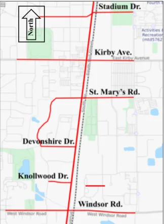
The study area consists of five intersections along the Neil Street corridor, Champaign, IL (Figure 2). At the time of data collection in Feb- March 2017, the five intersections on Neil Street were operating as time-based coordinated signals and provided progression for northbound and southbound traffic (the major street). Four of the crossing streets create typical four-legged intersections and one of them create three-legged intersection; including one Major Street and five Minor Streets. Schematic geometries of the five intersections are shown in Figures 3 through 7 (the drawings are not to scale) (Benekohal et al. 2018).

(18)

Figure 2: Five study intersections along the Neil Street corridor, Champaign, IL. (Stadium Dr., Kirby Ave., St. Mary’s rd., Devonshire Dr., Windsor Rd.) (Benekohal et al. 2018)

Figure 3: Geometry of the intersection of Neil Street and Stadium Drive.

N

or

(19)

Figure 4: Geometry of the intersection of Neil Street and Kirby Avenue.

Figure 5: Geometry of the intersection of Neil Street and St. Mary’s Road.

(20)

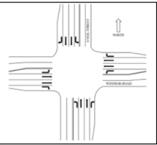
Figure 7: Geometry of the intersection of Neil Street and Windsor Drive.

3.2.2 Field Data Collection Methodology

During the Feb- March 2017, data collection was conducted by recording the online streaming traffic videos provided by the cameras at the five intersections. Two video sets of data were recorded in Feb-March 2017, during the morning peak (7:30-8:30 am), the noon peak (12:10-13:10 pm), and the afternoon peak (16:40 – 17:40 pm) hours in a day. The dates corresponding to the data collection at each intersection and data reduction are shown in Table 1 through Table 3.

Table 1: Feb-March 2017 data collection dates (Video set 1) Intersection AM Noon Peak PM

Stadium Feb 15, 2017 Feb 15, 2017 Feb 15, 2017 Kirby Feb 15, 2017 Feb 15, 2017 Feb 15, 2017

St Marys Feb 16, 2017 Feb 16, 2017 Feb 16, 2017/ Feb 22, 2017 Devonshire Feb 16, 2017 Feb 16, 2017 Feb 16, 2017/ Feb 22, 2017 Windsor Feb 28, 2017 Feb 28, 2017 Feb 28, 2017

Table 2: Feb-March 2017 data collection dates (Video set 2) Intersection AM Noon Peak PM

Stadium March 1, 2017 March 1, 2017 March 1, 2017 Kirby March 1, 2017 March 1, 2017 March 1, 2017 St Marys March 2, 2017 March 2, 2017 March 2, 2017

(21)

Table 3: Feb-March 2017 data reduction dates

Intersection AM Noon Peak PM

Stadium Feb 15, 2017 Feb 15, 2017 Feb 15, 2017

Kirby March 1, 2017/ Feb 15 2017 Feb 15, 2017 March 1, 2017 (NB, EB, WB) & Feb 15,2017 (SB) St Marys March 2, 2017 March 2, 2017 March 2, 2017

Devonshire March 2, 2017 March 2, 2017 March 2, 2017 Windsor March 7, 2017 March 7, 2017 Feb 28, 2017

3.2.3 Data Reduction

This chapter describes the methodology used for reducing the data elements from the traffic videos. Several types of characteristics data were extracted from the traffic videos and they are as follows: hourly volume, signal timing, field delay, and queue length. Data reduction was performed for the three time periods (am peak, noon peak and pm peak), see Table 3. In the following sections, a detailed description of data reduction, along with the outcomes for each item, are presented.

3.2.3.1 Signal Timing

The signal timing data was reduced in order to get the effective green time and cycle length data. The signal timing data are from the existing traffic control reports at the corresponding intersections.

3.2.3.2 Field Delay

The field measurement technique for intersection control delay, as described in HCM (2016), was adopted to calculate stopped delay per vehicle (the HCM procedure call it time in queue, as mentioned before) and control delay using the field videos. The measurements were carried out on a lane-group basis for each approach of the five intersections. The procedure was performed for all three time periods and the values are reported as cycle-by-cycle dvq values for

the three time periods and per all approaches.

The procedure requires identifying the approach speed during each study period. The speed limit of each approach in the field was assumed to be its approach speed for each intersection. The duration of the survey period was essentially equal to 1 hour for each peak hour and off-peak hour.

(22)

The count interval of 20 seconds was selected for this study because it is an integral divisor of the duration of survey period (1 hour) as required by the HCM (2016). As mentioned before, according to the Highway Capacity Manual;

d_V/ = WI_Y∑ V?/

V_\]\ ^ 0.9 (6)

dvq = Time-in-queue per vehicle (s/veh);

I_Y = Survey count interval (s) ∑ V?/ = Total vehicles in queue; V_\]\= Total vehicles arriving.

3.2.3.3 Queue Length

The queue lengths in the field were determined using the video images of the approaches. Based on the HCM (2016) procedure, the queue length of a through lane group of an intersection was determined by manually counting the number of stopped vehicles at the beginning of the green light. This counting also includes vehicles that joined the queue after the end of the red light, and came to a complete stop. The average queue data were calculated from the raw field data.

3.3 DESCRIPTION OF RAW DATA  

The outcome of the data collection is the input dataset in the methodology chapter of this study. The raw dataset includes cycle-by-cycle data at each approach (NB, SB, EB and WB), per all intersections along the corridor and during all three time periods (AM, NP, PM), which are all stored in a CSV file. The CSV file included 1860 rows and 6 columns. Each row represents the information for a cycle. All of the rows, 1860 observations, represent the total analysis period. Each column represents an attribute. The raw dataset includes the following attributes:

(23)

C: cycle Length (s); which is the total signal time to serve all of the signal phases including the green time plus any change interval. The dataset includes the cycle-by-cycle, cycle length information obtained from the signal timing plan for the entire corridor and time periods.

Q: queue length; this attribute is the number of vehicles stopped in a queue on a cycle-by-cycle basis. As explained previously, this data is obtained by field queue length measurement procedure presented by HCM (2016).

g: effective green time, is the time during which a given approach or set of approaches may proceed at the saturation flow rate; the dataset includes the cycle-by-cycle effective green time information obtained from the signal timing plan for the entire corridor and time periods.

(24)

CHAPTER 4: METHODOLOGY OF RESEARCH

A range of statistical and machine learning methods can be used for predicting purposes (Wu et al. 2004; Nabian et al. 2017). However, previous delay estimation studies have not been focusing on using statistical and machine learning models to predict vehicle delay at signalized intersections; this study presents a systematic and comprehensive evaluation and comparison between the performance of the three machine-learning models; Linear Regression (LR), Support Vector Machine Regression (SVR) and Regression Random Forest (RF), using the dataset described in the previous chapter in order to get an efficient and accurate vehicle delay prediction at a signalized intersection.

4.1 DATA PREPARATION AND CLEANING

A variety of data preparation and data cleaning tasks are usually necessary for organizing the inputs to any prediction model. The available raw dataset which is an outcome of a manual data reduction and includes 1860 data points (1860 cycles along a corridor), may consist of some errors and also might have meaningless inputs for the prediction models.

The dataset used in this study was filtered to be best suited to predicting vehicle delays. We exclude the observations with the dvq of zero but queue length of more than zero. We also

exclude the observations with the queue length of zero but dvq of more than zero. These excluded

observations are not making any reasonable sense for being inputted to a prediction model. This makes the input dataset to the prediction model including 1522 observation and 3 predictor variables and one response variable.

We have also further split the dataset to have three separate datasets for predictive modeling. First dataset includes of the major and minor streets data, second dataset includes the major street data and the third dataset includes the minor streets data.

(25)

Table 4: Explanation of the predictor variables and response variable in the dataset Predictor Variables Notation

X1: Cycle Length C

X2: Queue length per Cycle Q

X2: Effective Green Time per Cycle g

Response Variable Notation

Y: vehicle delay per cycle (time-in-queue per vehicle) dvq

4.1.1 Training and Testing Sets

Prediction by machine learning is performed through two stages: The first stage is training the model and the second stage is producing a result by prediction and testing them. To this end, each of the original datasets were randomly divided into two different datasets, one for training and one for testing. The training set is 70 percent of the original dataset and the rest 30 percent of the original dataset is the testing set (Tables 5 through 7).

The training data was further used to train the machine learning models to find the relationships between the predictors and the vehicle delays. Then, all of the generated models were tested by using the testing data to determine their accuracy. The error was calculated as the absolute value of the difference between the predicted delay (dvq) and the field delay (dvq). The average

error was then calculated.

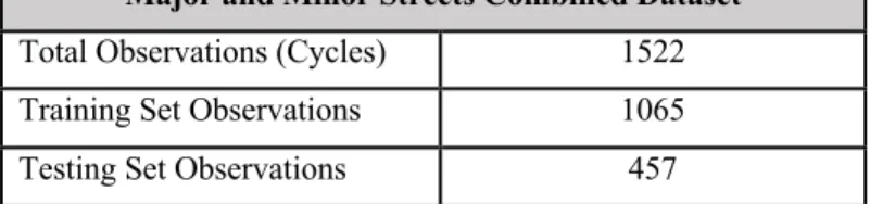
Table 5: Major and minor streets combined dataset for training and testing Major and Minor Streets Combined Dataset

Total Observations (Cycles) 1522 Training Set Observations 1065 Testing Set Observations 457

Table 6: Minor streets dataset for training and testing Major Streets Dataset

(26)

Table 7: Minor streets dataset for training and testing Minor Streets Dataset

4.2. PREDICTIVE MODELING 4.2.1 Linear Regression

Linear regression is an approach for modeling the relationship between a response variable and one or more predictor variables. Linear regression can be used to fit a predictive model to an observed data set of values of the response and predictor variables, if the goal of a study is prediction. The case with one predictor variable is called simple linear regression; and for more than one predictor variable, the process is called multiple linear regression. In general, Multiple Linear Regression given n observations, is in the form of:

y` = bb+ b&x& + b,x,+ ⋯ + b@x@ (7)

where 𝑦 gis the predicted response variable, x1 through xn are n distinct predictor variables, b0 is

the value of y when all of the predictor variables (X1, X2, …, Xn) are equal to zero; and

b1 through bn are the estimated regression coefficients. Each regression coefficient represents the

change in y relative to one unit of change in the respective response variable. In the multiple regression situation, b1, for example, is the change in y relative to a one-unit change in X1,

holding all other independent variables constant.

These models would assume a space of (-∞, +∞) for the response variable. The response variable in this study is vehicle delay and represents time in queue and is non-negative. So, for dealing with the situations in which the Multiple Linear Regression models yield negative predictions for response variables, we have set the negative predictions to zero.

(27)

4.2.2 Support Vector Machine

A Support vector machine (SVM) is a machine learning tool for classification and regression analysis, first developed by Vapnik (1995). Support vector machine regression (SVR) is considered as a non-parametric technique which relies on kernel functions and represents the mapping of observations in the input space into a high-dimensional feature space where linear regression can be applied. Therefore, a nonlinear model in the input space can be learned from a subset of observations (support vectors) by linear regression in the high-dimensional feature space. The following mathematical formulation is based on the documentation of the Statistics and Machine Learning Toolbox in MATLAB (2018).

4.2.2.1 Linear Support Vector Machine Regression (SVR): Primal Formula

When using Support Vector Machine in regression analysis (SVR), the Support Vectors use a cost function to measure the empirical risk of regression error minimization. Among many choices of the loss functions to calculate the cost, the MATLAB Statistics and Machine Learning Toolbox uses epsilon-insensitive loss function and implements epsilon-insensitive SVM (ε-SVM) regression. In ε-SVM regression, the set of training data includes predictor variables and the observed response variable. The purpose of ε-SVM regression is to find a function f(x) that deviates from yi by a value no greater than ε for each training point x, and at the same time is as

flat as possible.

Suppose we are given training data {(x1, y1), ..., (xk, yk)} ⊂ X × R, where X denotes the

space of the input patterns (e.g. X = Rd_{) To find the linear estimation function in SVR:}

f(x) = (w, x) + b with w ∈ X, b ∈ R (8)

Where (·,·) denotes the dot product in X. Flatness with regard to the Equation 8 means that the purpose is seeking for a small w. Minimizing the norm, i.e. ||w||2_{= (w,w),is one way to ensure}

the small w. This problem as a convex optimization problem could be defined: minimize &_,‖w‖,₍₉₎

Subject to qy_{(w, x}?− (w, x?) − b ≤ ε ?) + b − y? ≤ ε

(28)

Equation 9, implicitly assumes that such a function f, truly exists and approximates all pairs (xi, yi) with ε precision; in other words, the convex optimization problem is considered as feasible

(Smola et al. 2004).

However, sometimes this is not the case and one may want to allow some errors. Then, one can introduce slack variables ξi, ξi* to manage otherwise infeasible constraints of the optimization

problem (Equation 9). Thus, the formulation in Vapnik (1995) would be reached: minimize &_,‖w‖,_{+ C ∑ (ξ} ?+ ξ?∗) v ?w& (10) Subject tox y_?− (w, x_?) − b ≤ ε (w, x?) + b − y? ≤ ε ξ_?+ ξ_?∗_{≥ 0}

The constant C > 0 (Box Constraint) determines the trade-off between the flatness of the linear function f and the amount up to which deviations higher than ε are tolerated (defines penalties to estimation errors). This corresponds to dealing with a ε-insensitive loss function |ξ |ε as follows (Smola et al. 2004):

|ξ|{ ≔ q_{|ξ| − ε otherwise}0 if |ξ| ≤ ε (11)

As a tool, we have used MATLAB function ‘fitrsvm’ for implementing Support Vector Machine Regression modeling in this study. SVR results for all major and minor streets will be presented in the next chapter.

4.2.3 Random forest

Random forest (RF) is a machine learning method that generate many regression models and aggregate their results, first developed by Breiman (2001). RFs are tree-based regression models and its basic idea is partitioning the input space into a set of sub-samples of the data, and then fitting a simple model. In other words, RF modeling is carried out through constructing a multitude of decision trees in the training stage and outputting the mean prediction (regression) of

(29)

4.2.3.1Decision Tree

Decision tree is a non-parametric machine learning approach which is used for predictive modeling. Decision trees can be applied as classification trees and regression trees; and predict nominal (discrete) and numeric (continuous) values for the response variables, respectively. A decision rule is embedded in a decision tree, followed to get the prediction task done given a set of features. One approach to build the decision rules is following a sequence of simple tests, in which each test uses the results of all previous tests. This class of rules can be presented as a tree, where each node represents one test, and edges represent the possible outcome of each test.

To do the prediction task for a data point with a tree identified above, the first node is fed by the features of that data point, and then the outcome of the test performed in that node determines to which node it goes at the next iteration, and so on, until the data point reaches a leaf. Finally, the data point outcome is predicted using a voting or averaging action at the leaf nodes (Forsyth, 2018).

We start with a node at the root, then recursively split the data at that node, partitioning the data to the left and to the right, until we reach the nodes at the leaf (Forsyth, 2018). Splitting involves choosing a decision function to apply the best split for a node. The main questions in decision tree modeling are how to select the best split, and when to stop.

Splitting should be stopped when there is too little data at a node, since it is hard to pick a decision function with small amount of data. The model is prone to overfitting risk, if the tree is too deep. In that case, the model would be in trouble finding solution for a variety of problems. But if the tree is not too deep, model would result in more promising results even by using various data in the model. Therefore, in decision tree modeling, we are always searching for a model that is not too deep by using proper tree pruning, which means to stop creating the conditional splits in the right time and instead, choose a limiting feature and split threshold with a high information gain, at each tree node. Hence, to choose the best split threshold, we need to determine how much information gain is caused by the split (Forsyth, 2018).

Assume the training data vectors as xi ∈_{RI, i = 1···I, and a response variable vector y}∈ RO; where I and O are the input and output dimensionality respectively, a decision tree recursively

(30)

splits the input space in a way that the training data with similar values are grouped together. Let denote the data at node m by D.

For each splitting candidate θ = (f, tm), including the feature f and threshold tm, the data D

is partitioned into Dleft(θ) and Dright (θ) subsets:

Dvƒ„\(θ) = (x, y)|x„ ≤ t> (12) D_†?‡ˆ\(θ) = D\Dvƒ„\(θ) (13)

The impurity of the split at node m is computed using an impurity function, I( ), as follows: G(D, θ) =@‹Œ•Ž

•• I‘Dvƒ„\(θ)’ +

@“”(•

•• I 5D†?‡ˆ\(θ)6 (14)

For minimizing the impurity of the split, we choose parameters as follows: θ∗ _{= argmin}

—G(D, θ) (15)

Then, through a recursive procedure for subsets of Dleft(θ*) and Dright(θ*), one should

continue until reaching the maximum allowable depth:

N_>< min_š›\› or N_>= 1 (16)

Regression criteria  

Predicting the response variable as a continuous value (regression), for node m, with Nm

observations, the following criteria for determining thresholds for next splits are typically used: Mean Absolute Error (MAE): minimizes the l1 error; using median values at leaf nodes, and Mean Squared Error (MSE): minimizes the l2 error; using mean values at leaf nodes.

Following, the MAE and MSE equations are presented in Equation 17 and Equation 18, respectively:

(31)

𝐼(•ž):

&

ž∑ (𝑦¡ − 𝑦¢£)

,

¡Î•ž (18)

Where Dm is the training data in the node m; and 𝑦¢_£ = &

ž∑¡Î•ž(𝑦¡) .

Although deep decision trees might be prone to overfitting risk; RF prevents overfitting most of the time, by creating random sub-samples of the training dataset and constructing smaller trees using these sub-samples. Afterwards, it combines the trees trained on sub-samples. The efficiency of the model at this stage depends on how many trees the RF model constructs. Due to that, RF adds additional randomness to the model, while cerating the trees. Then instead of searching for the most important feature while splitting a node, its algorithm searches for the best feature among a random subset of features. This results generally results in a better model. 

As a tool, we have used MATLAB (2018) function ‘treebagger’ and chose regression as the method, for implementing RF regression in this study. RF regression results for all major and minor streets delay prediction will be presented in the next chapter

(32)

CHAPTER 5: DATA ANALYSIS AND FINDINGS

Using the training data with 3 predictor variables, for the combined dataset of major and minor streets, major street dataset and minor streets dataset, we trained LR, SVR model and RF regression model to predict the vehicle delay per cycle. In this chapter, first, we introduce a number of performance measures to evaluate the accuracy and efficiency of our prediction tasks. Second, we determine the structure of each machine-learning predictive model applied to our datasets. 5.1 PREDICTION PERFORMANCE TESTS

To evaluate the effectiveness of the proposed models and quantifying the quality of predictions, we use four performance indexes, which are the mean relative error (MRE) which we are defining the average prediction accuracy by (1-MRE); mean absolute error (MAE) and the root mean squared error (RMSE). They are defined as (Lv et al. 2015):

MRE = ∑¨”©7|§”'§g”|

∑¨”©7§” (19)

MAE = &_@ ∑@ |y_?− y`_?|

?w& (20) RMSE = [ _@& ∑ (|y@ _?− y`_?|),_]

?w&

7

+₍₂₁₎

Where y is the observed vehicle delay in the field, and y` is the predicted vehicle delay per cycle. Additionally, we will provide the plots of the cumulative distribution function (CDF) of the absolute error (AE) term in the prediction for all three models and conditions that is:

(33)

5.2 PREDICTIVE MODELS TRAINING AND PREDICTION 5.2.1 Linear Regression

5.2.1.1 Determination of the Structure of Linear Regression Model (Combined Dataset)

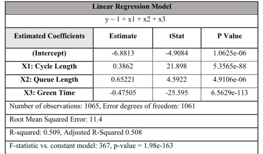
By training a Linear Regression model (LR), we predicted vehicle delay per cycle for the combined dataset (457 observations). The model specifications are presented in the Table 8:

Table 8: LR specifications (combined dataset) Linear Regression Model

y ~ 1 + x1 + x2 + x3

Estimated Coefficients Estimate tStat P Value

(Intercept) -6.8813 -4.9084 1.0625e-06

X1: Cycle Length 0.3862 21.898 5.3565e-88

X2: Queue Length 0.65221 4.5922 4.9106e-06

X3: Green Time -0.47505 -25.595 6.5629e-113

Number of observations: 1065, Error degrees of freedom: 1061 Root Mean Squared Error: 11.4

R-squared: 0.509, Adjusted R-Squared 0.508

F-statistic vs. constant model: 367, p-value = 1.98e-163

Based on the Table 8, in the model, all of the three explanatory variables are significant. Cycle length and queue length have positive values and the coefficient for green time is negative; this is acceptable since there could be an inverse relationship between green time and vehicle delay, specifically on minor streets.

In Table 8, we can also see that the R-squared value is 0.5; this value in Multiple Linear Regression, shows the goodness of fit for the regression model; i.e the predictors in the model explain 50% of the variability of the response variable.

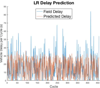
Figure 8 shows the output of the LR predicted vehicle delays per cycle during a total of 457 cycles. This figure includes the observed field delays for comparison. In Figure 8, it is shown that the predicted vehicle delays have similar patterns with the observed vehicle delays in the field.

(34)

Figure 8: A comparison between LR predicted and field vehicle delay on a cycle-by-cycle basis (combined dataset)

As another way of demonstrating the LR prediction performance, Figure 9 also compares the LR predicted and field vehicle delay on a cycle-by-cycle basis; as much as the data points are closer to the x=y line, the prediction tends to be more accurate (Nabian et al. 2018):

(35)

As shown in Figure 9, the for the field delays lower than 30 second, are mostly underestimated and the delays higher than 30, are mostly overestimated.

5.2.1.2Determination of the Structure of Linear Regression Model (Major Street Dataset)

By training a Linear Regression model (LR), we predicted vehicle delay per cycle for 260 observations (cycles). The model specifications are presented in the Table 9:

Table 9: LR specifications (major street dataset) Linear Regression Model

y ~ 1 + x1 + x2 + x3

Estimated Coefficients Estimate tStat P Value

X1: Cycle Length 0.109 8.9499 4.3672e-18

X2: Queue Length 1.715 16.714 8.2298e-52

X3: Green Time -0.15657 -8.5296 1.1864e-16

F-statistic vs. constant model: 315.4, p-value = 4.3121e-123

Based on the Table 9, in the model, all of the three explanatory variables are significant. This model does not have an intercept; since at the first stage of training this model, intercept was not significant; therefore, we trained a new LR model and eliminated the intercept from the model. Now, all of the model parameters are significant as shown in Table 9. Cycle length and queue length have positive values and the coefficient for green time is negative; this is acceptable since there could be an inverse relationship between green time and vehicle delay.

In Table 9, we can also see that the R-squared value is 0.61; this value in Multiple Linear Regression, shows the goodness of fit for the regression model; i.e the predictors in the model explain around 61% of the variability of the response variable.

Figure 10 shows the output of the LR predicted vehicle delays per cycle during a total of 260 cycles. This figure includes the observed field delays for comparison. In Figure 10, it is shown that the predicted vehicle delays on major street dataset have a closer similarity patterns with the

(36)

observed vehicle delays in the field rather than the LR predicted vehicle delays in the combined dataset.

Figure 10: A comparison between LR predicted and field vehicle delay on a cycle-by-cycle basis (major street dataset)

It could be a sign that our models are approach-sensitive (approach; major street or minor street approaches), since the prediction modeling performance for vehicle delay on the major street dataset individually, is significantly different than the prediction modeling performance on the major and minor streets combined dataset.

As another way of demonstrating the LR prediction performance, Figure 11 also

compares the LR predicted and field vehicle delay on a cycle-by-cycle basis; as much as the data points are closer to the x=y line, the prediction tends to be more accurate:

(37)

Figure 11: A visual display of the performance of the LR (major street dataset) In Figure 11, it is demonstrated that the accuracy of the vehicle delay prediction is in a satisfactory agreement.

5.2.1.3Determination of the Structure of Linear Regression Models (Minor Streets Dataset)

By training a Linear Regression Model (LR), we predicted vehicle delay per cycle for the combined dataset (197 observations). The model specifications are presented in the Table 12:

Table 10: LR specifications (minor streets dataset) Linear Regression Model

y ~ 1 + x1 + x2 + x3

Estimated Coefficients Estimate tStat P Value

(Intercept) -12.401 -4.1761 3.5559e-05

X1: Cycle Length 0.54372 15.95 8.2003e-46

X2: Queue Length 0.8005 2.8276 0.004896

X3: Green Time -0.91845 -11.129 1.3148e-25

(38)

Based on the Table 10, in the model, all of the three explanatory variables are significant. Cycle length and queue length have positive values and the coefficient for green time is negative; this is acceptable since there could be an inverse relationship between green time and vehicle delay, specifically on minor streets.

In Table 10, we can also see that the R-squared value is 0.42; this value in Multiple Linear Regression, shows the goodness of fit for the regression model; i.e the predictors in the model explain 42% of the variability of the response variable.

Figure 12 shows the output of the LR predicted vehicle delays per cycle during a total of 197 cycles. This figure includes the observed field delays for comparison. In Figure 12, it is shown that the predicted vehicle delays do not have reasonably similar patterns with the observed vehicle delays in the field.

Figure 12: A comparison between LR predicted and field vehicle delay on a cycle-by-cycle basis (minor streets dataset)

(39)

Figure 13: A visual display of the performance of the LR (minor streets dataset) In the Figure 13, it is evident that the LR is underestimating the vehicle delays below 30 seconds and overestimating the vehicle delays of higher than 30 seconds.

5.2.2 Support Vector Machine Regression Models

5.2.2.1 Determination of the Structure of Support Vector Machine Model (Combined Dataset)

Support Vector Machine Regression (SVR), as a nonlinear regression method, requires the specification of parameters related to its model architecture. Determining those parameters yielding robust regression models for our study, is challenging. Efficiency and accuracy of the predictions by SVR is influenced by the choice of two parameters, 𝜖 and C, and the choice of kernel functions. The parameter 𝜖 sets the limit of the deviation of the regression solution from training data in the input space. However, the limit set by 𝜖 is not strict since observations exceeding the limit will also be “tolerated” (i.e. included in the regression process) as long as they are within the limit of deviation set by the box constraint C. We have searched for hyperparameters that minimize the five-fold cross-validation loss, by automatic hyperparameter optimization using ‘fitrsvm’ function in MATLAB (2018). The optimization problem searches over Box Constraint, Kernel Scale, and Epsilon. The output is the regression with the minimum estimated cross-validation loss. Table 11 presents the SVR optimized hyperparameters:

(40)

Table 11: SVR optimized hyperparameters (combined dataset)

Support Vector Machine Specifications

Box Constraint (C) Kernel Scale Kernel Function Epsilon

828.18 64.885 Linear 0.86103

Figure 14 shows the output of the SVR predicted vehicle delays per cycle during a total of 457 cycles. This figure includes the observed field delays for comparison.

Figure 14: A comparison between SVR predicted and field vehicle delay on a cycle-by-cycle basis (combined dataset)

In Figure 14, it is shown that the model is unable to keep the trend of prediction for the delays more than about 20 seconds.

(41)

Figure 15: A visual display of the performance of the SVR (combined dataset)

As shown in Figure 15, the predictions from delays more than 20 second, are getting less accurate. This might be due to lack of training delay data with the value of 20 seconds and more.

5.2.2.2 Determination of the Structure of Support Vector Machine (Major Street dataset)

Support Vector Machine Regression (SVR), as a nonlinear regression method, requires the specification of parameters related to its model architecture. Determining those parameters yielding robust regression models for our study, is challenging.

Efficiency and accuracy of the predictions by SVR is influenced by the choice of two parameters, 𝜖 and C, and the choice of kernel functions. The parameter 𝜖 sets the limit of the deviation of the regression solution from training data in the input space. However, the limit set by 𝜖 is not strict since observations exceeding the limit will also be “tolerated” (i.e. included in the regression process) as long as they are within the limit of deviation set by the box constraint C. We have searched for hyperparameters that minimize the five-fold cross-validation loss, by automatic hyperparameter optimization using ‘fitrsvm’ function in MATLAB (2018). The optimization problem searches over Box Constraint, Kernel Scale, and Epsilon. The output is the regression with the minimum estimated cross-validation loss. Table 12 presents the SVR optimized hyperparameters:

(42)

Table 12: SVR optimized hyperparameters (major street dataset)

Support Vector Machine Specifications

Box Constraint (C) Kernel Scale Kernel Function Epsilon

1.1756 0.71101 Linear 2.5848

Figure 16: A comparison between SVR predicted and field vehicle delay on a cycle-by-cycle basis (major street dataset)

As another way of demonstrating the SVR prediction performance, Figure 17 also compares the SVR predicted and field vehicle delay on a cycle-by-cycle basis; as much as the data points are closer to the x=y line, the prediction tends to be more accurate:

(43)

Figure 17: A visual display of the performance of the SVR (major street dataset)

5.2.2.3 Determination of the Structure of Support Vector Machine Model (Minor Streets Dataset)

Support Vector Machine Regression (SVR), as a nonlinear regression method, requires the specification of parameters related to its model architecture. Determining those parameters yielding robust regression models for our study, is challenging. Efficiency and accuracy of the predictions by SVR is influenced by the choice of two parameters, 𝜖 and C, and the choice of kernel functions. The parameter 𝜖 sets the limit of the deviation of the regression solution from training data in the input space. However, the limit set by 𝜖 is not strict since observations exceeding the limit will also be “tolerated” (i.e. included in the regression process) as long as they are within the limit of deviation set by the box constraint C. We have searched for hyperparameters that minimize the five-fold cross-validation loss, by automatic hyperparameter optimization using ‘fitrsvm’ function in MATLAB (2018). The optimization problem searches over Box Constraint, Kernel Scale, and Epsilon. The output is the regression with the minimum estimated cross-validation loss. Table 13 presents the SVR optimized hyperparameters:

(44)

Table 13: SVR optimized hyperparameters (minor streets dataset) Support Vector Machine Specifications

Box Constraint (C) Kernel Scale Kernel Function Epsilon

15.067 2.9537 Linear 3.8777

Figure 18: A comparison between SVR predicted and field vehicle delay on a cycle-by-cycle basis (combined dataset)

As another way of demonstrating the SVR prediction performance, Figure 19 also compares the SVR predicted and field vehicle delay on a cycle-by-cycle basis; as much as the data points are closer to the x=y line, the prediction tends to be more accurate:

(45)

Figure 19: A visual display of the performance of the SVR (minor streets dataset)

5.2.3 Regression Random Forest Models

5.2.3.1 Determination of the Structure of Regression Random Forest Model (Combined Dataset)

Predictive modeling by RF regression requires the specification of the maximum number of features used for data partition when looking for the best split in tree regressions and the number of tree regressions used for averaging.

In this study, the maximum number of features is taken to be the number of explanatory variables (i.e. 3), and the number of tree regressions is chosen to be 15. Empirical tests show that there is no evident improvement in prediction accuracy of vehicle delay when the number of tree regressions in RF is larger than 15. We use mean squared error in order to specify the optimal number of trees. Figure 20 shows the output of the RF predicted vehicle delays per cycle during a total of 457 cycles. This figure includes the observed field delays for comparison. In Figure 20, it is shown that the predicted vehicle delays have pretty similar patterns with the observed vehicle delays in the field.

(46)

Figure 20: A comparison between RF predicted and field vehicle delay on a cycle-by-cycle basis (combined dataset)

As another way of demonstrating the RF prediction performance, Figure 21 also compares the RF predicted and field vehicle delay on a cycle-by-cycle basis; as much as the data points are closer to the x=y line, the prediction tends to be more accurate:

(47)

5.2.3.2 Determination of the Structure of Random Forest (Major Street Dataset)

Predictive modeling by RF regression requires the specification of the maximum number of features used for data partition when looking for the best split in tree regressions and the number of tree regressions used for averaging.

In this study, the maximum number of features is taken to be the number of explanatory variables (i.e. 3), and the number of tree regressions is chosen to be 5. Empirical tests show that there is no evident improvement in prediction accuracy of vehicle delay when the number of tree regressions in RF is larger than 5. We use mean squared error in order to specify the optimal number of trees (Figure…).

Figure 22 shows the output of the RF predicted vehicle delays per cycle during a total of 260 cycles. This figure includes the observed field delays for comparison. The results are shown to be in a satisfactory agreement since the predicted vehicle delays have pretty similar patterns with the observed vehicle delays in the field.

Figure 22: A comparison between RF predicted and field vehicle delay on a cycle-by-cycle basis (combined dataset)

(48)

As another way of demonstrating the RF prediction performance, Figure 23 also

compares the RF predicted and field vehicle delay on a cycle-by-cycle basis; as much as the data points are closer to the x=y line, the prediction tends to be more accurate:

Figure 23: A visual display of the performance of the RF (major street dataset)

5.2.3.3 Determination of the Structure of Random Forest Model (Minor Streets Dataset)

Predictive modeling by RF Regression requires the specification of the maximum number of features used for data partition when looking for the best split in tree regressions and the number of tree regressions used for averaging.

In this study, the maximum number of features is taken to be the number of explanatory variables (i.e. 3), and the number of tree regressions is chosen to be 20. Empirical tests show that there is no evident improvement in prediction accuracy of vehicle delay when the number of tree regressions in RF is larger than 20. We use mean squared error in order to specify the optimal number of trees.

(49)

Figure 24: A comparison between RF predicted and field vehicle delay on a cycle-by-cycle basis (minor streets dataset)

As another way of demonstrating the RF prediction performance, Figure 25 also

compares the RF predicted and field vehicle delay on a cycle-by-cycle basis; as much as the data points are closer to the x=y line, the prediction tends to be more accurate:

(50)

CHAPTER 6: ANALYSIS OF THE RESULTS AND DISCUSSION

6.1 ANALYSIS AND DISCUSSION

The outputs of the applied models for the vehicle delay prediction of the combined major and minor streets dataset, major street dataset and minor streets dataset are presented. Now, a comprehensive comparison between the performance of the three models used in this study will be demonstrated. Finally, a discussion is provided to highlight the effectiveness the best predictive model for vehicle delay prediction when compared to other existing models.

In the previous chapter, it has been shown through the figures that the predicted vehicle delays have similar patterns with the observed vehicle delays in the field. In addition, it matches well on major street condition. However, the proposed model does not perform well on minor streets.

Table 14: Performance comparison of the MAE, the RMSE and the MRE for LR, the SVR and the RF

We compared the performance of the three models; Linear Regression (LR), support vector machine regression (SVR) and regression random forest (RF). Among these three competing methods, the LR and RF method are relatively the most effective and accurate models for prediction. In all cases, we used the same data set. The prediction results on the test data sets are given in Table 14.

For the combined dataset, the RF showed the best prediction accuracy (1-MRE) of 61%. The prediction errors (MAE:6.00 and RMSE:8.66) for RF are also the lowest among the three

Task

Linear Regression Support Vector Machine Random Forest MAE RMSE MRE MAE RMSE MRE MAE RMSE MRE Major and Minor Delay Prediction1 ₇ _9.81 _0.45 _7.01 _10.67 _0.46 _6.004 _8.66 _0.39 Major Street Delay Prediction 3.15 5.30 0.37 3.25 5.43 0.36 3.09 5.28 0.35

(51)

the highest among the three models. Also, the R-squared for the LR is 0.5 which shows that the predictors in the model are able to explain 50% of the variation in the response variable.

For the major street dataset, the RF showed the best prediction accuracy (1-MRE) of 65%. The prediction errors (MAE:3.09 and RMSE:5.28) for RF are also the lowest among the three models. SVR, is standing in the second stage in prediction accuracy, after RF, with prediction accuracy of 64%. The prediction errors (MAE:3.25 and RMSE:5.43) for SVR are also lower than LR and more than RF. LR, proved to have the worst accuracy in the major street dataset, with an average accuracy of 63%. The prediction errors (MAE:3.15 and RMSE:5.30) for LR are also the highest among the three models. Also, the R-squared for the LR is 0.61 which shows that the predictors in the model are able to explain around 61% of the variation in the response variable. The R-squared value for the major street dataset is higher than that of combined dataset (0.50).

For minor streets dataset, the RF showed the best prediction accuracy (1-MRE) of 55%. The prediction errors (MAE:9.9 and RMSE:13.00) for RF are also the lowest among the three models. LR, is standing in the second stage in prediction accuracy, after RF, with prediction accuracy of 51%. The prediction errors (MAE:10.91 and RMSE:13.95) for LR are also lower than SVR and more than RF. SVR, proved to have the average prediction accuracy of 51%, similar to LR. Although, the prediction errors (MAE:10.83 and RMSE:13.96) for SVR are slightly higher than LR. Also, the R-squared for the LR is 0.42 which shows that the predictors in the model are able to explain around 42% of the variation in the response variable. The R-squared value for the minor street dataset is less than that of combined dataset (0.50) and the major street dataset (0.61). In Table 14 we can find that the LR and RF proved to be reasonably accurate for the prediction of the vehicle delay per cycle. This prediction accuracy is promising, robust, and comparable with the reported results. The most accurate results yielded by LR and RF, are for the major street vehicle delay prediction. Notice that we only use the vehicle delay per cycle data as the input for prediction without considering other engineering factors, such as weather conditions, accidents, and other vehicle delay parameters (volume, speed; etc) that have a relationship with the vehicle delay.

As a visual display of the performance we plot the cumulative distribution function (CDF) of the absolute error term in the prediction that is |y_?− y`_?|, for the three models in the study for the combined dataset, major street dataset and minor streets dataset conditions in Figures 26 (a-c).

(52)

The RF model leads to improved vehicle delay prediction performance when compared with LR and SVR, by reducing the absolute error in prediction in all three conditions. Although, it is evident that for the major street dataset, all three models are closely competing and there is only some slight difference between their performances and prediction accuracies.

Figure 26 (a-c): CDFs of absolute error in the prediction for the three models (x=|𝑦_¡− 𝑦`_¡|) For the RF, the average accuracy is 61%, 65% and 55% for the combined dataset, major street dataset and minor streets dataset tasks, respectively.

(a) (b)

(53)

was 55%, 63% and 51% for the combined dataset, major street dataset, and minor streets dataset, respectively.

Furthermore, prediction results on major street showed that, LR had errors less than 6 seconds in 87% of the predictions; SVR also had errors less than 6 seconds in 87% of the predictions; and RF had an errors less than 6 seconds in 80% of the predictions. Thus, the effectiveness of the LR method (which is a straightforward model to use) for vehicle delay prediction on major street is promising and manifested.

6.2 ACCURACY IMPROVEMENT PROCEDURES

As one way of demonstrating the prediction performance in Chapter 4, the scatter plots of the predicted vehicle delay values by the models versus the field vehicle delay values were presented. The prediction accuracy of the model is in the satisfactory agreement if the points in these scatter plots are closer to the line of x=y.

As a possible diagnosis and taking a closer look to the problem, we have found out that the lack of data could result in some issues in the shape of these scatter plots and thus, in the predictions for all of the models. As an example, in Figure 27 (a-b), we are contrasting the histogram plot of the field delays (observations) and the plot for the LR prediction performance in the combined dataset which compares the LR predicted and field vehicle delay on a cycle-by-cycle basis. It is evident that the prediction accuracy of the model is higher in where more observations exist, and the accuracy drops where the data points are not sufficient. Also, the model is underestimating the delay for the field delay values of lower than 30 seconds and overestimating for the higher than that:

Figure 27 (a-b): Contrasting the performance of the LR for the combined dataset with the number of observations for each field delay value

(54)

According to the Figure 9, we would expect that removing the observations with the less frequent values (as a threshold, we could consider frequencies below 60), could improve the prediction accuracy. In this case, for the example above, we removed the field delay observations with the values more than 30 seconds (as their frequency is below 60) and trained a LR on the new dataset.

Figure 28 (a-b): Contrasting the performance of the LR for combined dataset with the number of observations for each field delay value (removing field delay values > 30 seconds)

Figure 28 presents the results of training the LR on the new dataset with removed observations with frequency below 60. We can see that the prediction accuracy of LR is improved. This diagnosis with similar reasoning would be extended to all of the other prediction models in this study. Since we are witnessing improvement in the predictions by removing less frequent field delay values in the dataset, one can conclude that the even frequencies of the field delay values, is essential for more accurate prediction outcomes.

6.3 FURTHER ANALYSIS ON THE MAJOR STREET DATASET

Based on the predictions resented in the previous sections, it is demonstrated that all of the three models are yielding promising results on the major street. For the purpose of proposing further improvements in the predictive models, in this section presents a further detailed analysis and models fine-tunings on the major street dataset.

(55)

6.3.1 Diagnosis for the Negative Predictions on the Major Street

In the previous sections is was explained that the linear regression model would yield values for the response variable in the space of (-∞, +∞); hence in the modeling vehicle delay predictions we set the negative LR predicted values to zero.

In the LR model equation on the major street, the intercept and the coefficient of the predictor variable X3, effective green time, are negative. Hence, logically the negative values for

the predicted delays are due to the negative intercept and X3 coefficient. So, high values of X3 can

force the model in predicting negative values for the response variable (delay).

Effective green time for