Case study on bagging stable classifiers for data streams

(1)

Case Study on Bagging Stable Classifiers for Data Streams

Abstract

Ensembles of classifiers are among the strongest classi-fiers in most data mining applications. Bagging ensembles exploit the instability of base-classifiers by training them on different bootstrap replicates. It has been shown that Bagging instable classifiers, such as decision trees, yield generally good results, whereas bagging stable classifiers, such ask-NN, makes little difference. However, recent work suggests that this cognition applies to the classical batch data mining setting rather than the data stream setting. We present an empirical study that supports this observation.

1. Introduction

Ensembles of classifiers are among the strongest classi-fiers in most data mining applications. By building multiple different models and combining the predictions of those, predictive accuracy typically improves over building just one model. Some well known ensemble techniques are Bagging [6], Boosting [18] and Stacking [10, 24]. Bagging exploits the instability of classifiers. The base-classifiers are trained on slightly different samples of the training set, yielding diverse models. Common decision tree induction algorithms are known to be instable, which makes them appropriate to be used in a bagging ensemble. Classifiers such as Naive Bayes andk-Nearest Neighbour are known to bestable, slight changes in the training set do not in-fluence predictions. Breiman already showed that Bagging

k-Nearest Neighbour does not yield accuracy improvement, when used in a classical batch data mining setting.

However, it is unknown whether this observation holds in the data stream setting. Data stream mining varies from the batch classification setting in various ways [3, 4, 11, 17, 20]. In the conventional batch setting, a finite amount of sta-tionary data is provided and the goal is to build a model that fits the data as well as possible. When working with data streams, we should expect an infinite amount of data, where observations come in one by one and are being processed in that order. Furthermore, the nature of the data can change over time, known asconcept drift. Classifiers should be able to detect when a learned model becomes obsolete and

up-date it accordingly. All of these differences are not covered by the original work on Bagging [6].

In [20] some observations were reported that suggest that Bagging stable classifiers in the data stream setting actually does improve accuracy, even though gains are small. In this paper, we study the effect of bagging stable classifiers in the data stream setting. Our contribution is empirical evidence that suggests that bagging stable classifiers does improve predictive performance on data streams. Although the per-formance gains that can be obtained are small, this result can be seen as a form of meta-knowledge. It adds to the knowledge of how classifiers behave and what classifiers to use on what data. All results are made publicly available in OpenML [19, 22].

2. Related Work

The requirements for processing streams of data are: process one example at a time (and inspect it only once), use a limited amount of time and memory, and be ready to pre-dict at any point in the stream [3, 17]. These requirements inhibit the use of most batch data mining algorithms. How-ever, some algorithms can trivially be used or adapted to be used in a data stream setting, for example, NaiveBayes [15],

kNearest Neighbour (k-NN) [1, 25], and Stochastic Gradi-ent DescGradi-ent [5]. Also, many algorithms have been created specifically to operate on data streams. Most notably, the Hoeffding Tree [9] is a tree based algorithm that splits the data based on information gain, but uses only a small sam-ple of the data determined by the Hoeffding bound. The Hoeffding bound gives an upper bound on the difference between the mean of a variable estimated after a number of observations and the true mean, with a certain probabil-ity [13].

Ensembles of classifiers are among the best performing learning algorithms in the traditional batch setting. Mul-tiple models are produced that all vote for the label of a certain instance. The final prediction is made according to a predefined voting schema, e.g., the class with the most votes wins. In [12] it is proven that the error rate of an en-semble in the limit converges to the Bayes error rate if two conditions are met: first, the individual models must do bet-ter than random guessing, and second, the individual

(2)

mod-els must be diverse, meaning that their errors should not be correlated. For example, Bagging [6] exploits the instability of classifiers by training them on differentbootstrap repli-cates: resamplings (with replacement) of the training set. Effectively, the training sets for various classifiers differ by the weights of their training examples. Two variants of Bag-ging have been designed specifically for the data stream set-ting. Online Bagging[16] draws the weight of each exam-ple from aPoisson(1)distribution, which converges to the behavior of the classical Bagging algorithm if the number of examples is large. Leveraging Baggingdraws the weights of each example from aPoisson(λ)distribution, whereλis a parameter under the user’s control (default value6). Fur-thermore, the ensemble is equipped with the ADWIN drift detection method [2], making sure that obsolete ensemble members are replaced with new ones. Although Leveraged Bagging differs from classical Bagging techniques, it seems to work very well in practise [4, 20].

3. Experimental Setup

We will compare the predictive accuracy of stable clas-sifiers with their accuracy when used in a bagged ensemble. We selected Naive Bayes andk-NN, as both are known to be stable classifiers [21], and have implementations available in the MOA framework [3]. k-NN seems to behave more stable with a higher value fork. We setk= 10, since this seems to be fairly stable. As for the Bagging techniques, we include both Online Bagging and Leveraging Bagging. Online Bagging is the most objective Bagging technique. Leveraging Bagging also includes a change detector, hence performance gains obtained by Leveraged Bagging schemas can be due to the change detector. The differences in accu-racy are tested for significance using a Paired T-Test and the Wilcoxon Signed-Ranks Test, both explained in [8]. Note that when comparing multiple classifiers with each other, ideally a test suited for multiple classifiers should be used, e.g., the Nemenyi test. However, in this case we are only interested in the impact of bagging on the performance of these classifiers.

We use all data streams that are available in OpenML [22]. These cover both real world data streams and synthetically generated data streams, as is common in data stream literature [4, 17, 20]. We discuss a few of them in more detail.

SEA Concepts The SEA Concepts Generator generates three numeric attributes from a given distribution, of which only the first two are relevant. The class that needs to be predicted is whether these values exceed a certain thresh-old. Several SEA Concept generated data streams based on different data distributions can be joined together in order to simulate concept drift.

STAGGER The STAGGER Concepts Generatorgener-ates descriptions of geometrical objects. Each instance de-scribes the size, shape and color of such object. A STAG-GER concept is a binary classification rule distinguishing between the two classes, e.g., all blue rectangles belong to the positive class.

Rotating Hyperplanes The Rotating Hyperplane Gen-erator [14] generates a high-dimensional hyperplane. In-stances represent a point in this high-dimensional space. The task is to predict whether such a point is within the hy-perplane. Concept drift can be introduced by rotating and moving the hyperplane.

LED The LED Generator [7] generates instances based on a LED display. Attributes represent the various LED lights, and the task is to predict which digit is represented. In order to add noise, attributes can display the wrong value with a certain probability. Furthermore, additional (irrele-vant) attributes can be added.

Random RBF The Random RBF Generator generates a number of centroids. Each has a random position in Eu-clidean space, standard deviation, weight and class label. Each example is defined by its coordinates in Euclidean Space and a class label referring to a centroid close by. Cen-troids move at a certain speed, generating gradual concept drift.

Bayesian Network The Bayesian Network Genera-tor [20] takes a batch data set as input, build a Bayesian Network over it, and generates instances based on the prob-ability tables. As the Bayesian Network does not change over time, it is unlikely that a native form of concept drift occurs in the data stream. The parameter set is the data set that was taken as input.

Composed Data Streams Common batch datasets can be appended to each other, forming one combined dataset cov-ering all observations and attributes, containing small peri-ods or abrupt concept drift. This is commonly done with the Covertype, Pokerhand and Electricity dataset [4, 17]. We applied a similar merge to the Airlines, CodeRNA and Adult dataset, forming “AirlinesCodernaAdult”. The origi-nal datasets are normalized before this operation is applied. IMDB.drama The IMDB dataset contains 120,919

movie plots. Each movie is represented by a bag of words of the globally1,000most occurring words. Originally, it is a multi-label dataset, with binary attributes whether it falls in a given genre. We predict whether it is in the drama genre, which is the most frequently occurring [17].

(3)

-0.004 -0.002 0 0.002 0.004 0.006 0.008

Agrawal1BNG(ionosphere)codrnaNormBNG(labor)AirlinesCodrnaAdultairlinesBNG(hepatitis)BNG(segment)BNG(cmc)BNG(credit-a)BNG(vote)BNG(trains)BNG(waveform-5000)RandomRBF(50;0.001)BNG(mushroom)BNG(soybean)Stagger3Stagger2Stagger1covertypeRandomRBF(0;0)RandomRBF(10;0.0001)BNG(anneal)BNG(spambase)RandomRBF(10;0.001)BNG(page-blocks)BNG(satimage)BNG(vowel)RandomRBF(50;0.0001)BNG(eucalyptus)BNG(solar-flare)IMDB.dramaBNG(zoo)SEA(50)BNG(dermatology)BNG(tic-tac-toe)BNG(SPECT)SEA(50000)BNG(wine)BNG(heart-statlog)BNG(heart-c)LED(50000)BNG(bridges_version1)BNG(pendigits)BNG(lymph)BNG(credit-g)BNG(JapaneseVowels)adultBNG(optdigits)Hyperplane(10;0.001)Hyperplane(10;0.0001)BNG(vehicle)electricityBNG(kr-vs-kp)BNG(colic.ORIG)BNG(letter)BNG(sonar)20_newsgroups.driftvehicleNormBNG(mfeat-fourier)CovPokElecpokerhand

Accuracy Difference

diff(Lev Bagging kNN,kNN)

(a) Leveraged Baggingk-NN Vs.k-NN

-0.2 -0.1 0 0.1 0.2 0.3 0.4 0.5 0.6

BNG(letter)BNG(vowel)BNG(bridges_version1)BNG(eucalyptus)BNG(colic.ORIG)BNG(mfeat-fourier)RandomRBF(10;0.001)Agrawal1BNG(page-blocks)BNG(credit-g)adultBNG(optdigits)BNG(solar-flare)BNG(heart-statlog)BNG(credit-a)BNG(sonar)BNG(hepatitis)BNG(spambase)BNG(heart-c)BNG(wine)Stagger1Stagger2BNG(JapaneseVowels)BNG(dermatology)Stagger3BNG(ionosphere)BNG(trains)BNG(labor)BNG(waveform-5000)BNG(mushroom)BNG(soybean)BNG(lymph)BNG(zoo)BNG(satimage)BNG(SPECT)BNG(pendigits)BNG(vote)BNG(kr-vs-kp)BNG(cmc)BNG(anneal)vehicleNormBNG(vehicle)codrnaNormBNG(segment)RandomRBF(0;0)BNG(tic-tac-toe)RandomRBF(10;0.0001)IMDB.dramaHyperplane(10;0.0001)airlinesSEA(50)SEA(50000)AirlinesCodrnaAdultelectricitypokerhandHyperplane(10;0.001)LED(50000)covertypeRandomRBF(50;0.001)RandomRBF(50;0.0001)20_newsgroups.driftCovPokElec

Accuracy Difference

diff(Lev Bagging NB,NaiveBayes)

(b) Leveraged Bagging Naive Bayes Vs. Naive Bayes

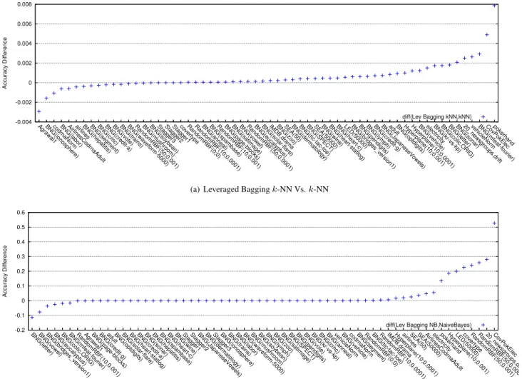
Figure 1. Performance differences between Leveraging Bagging ensemble and single classifiers.

20Newsgroups The original20Newsgroup dataset con-tains 19,300 newsgroup messages, each represented as a bag of words of the 1,000 most occurring words. Each instance is part of at least one newsgroup. This data set is commonly converted into20binary classification prob-lems, with the task to determine whether an instance be-longs to a given newsgroup. We append these data sets to each other, resulting in one large binary-class dataset con-taining386,000records with19shifts in concept [17].

4. Results

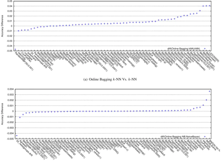
Figure 1 and Figure 2 show the result of the experiments. The x-axis shows the dataset, the y-axis shows the differ-ence in performance between the bagging schema and the single classifier. Note that the single classifier performed better on datasets where the difference is below zero, and vice versa for datasets where the difference is above zero.

Datasets are ordered by this difference. For full reference, Table 3 contains all results.

Figure 1(a) shows a similar trend as seen in the figure presented in [20]. There are few data streams on whichk -NN performs best, but many data streams on which Lever-aging Baggingk-NN performs best. A similar trend can be seen in the other figures.

One notable observation is the difference in scale be-tween on one hand Figure 1(b) describing the effect of using Naive Bayes in a Leveraging Bagging schema and the other figures. In most cases, the effect of a Bagging schema can attribute to performance gains of few percentages. How-ever in the case of LHow-everaged Bagging Naive Bayes, the performance gain can lead up to 50% (CovPokElec), but also other data sets show eminent improvements.

Among the 15data streams on which Leveraged Bag-ging improves upon Naive Bayes the most, many presum-ably contain concept drift (see Section 3). Compared to

(4)

-0.05 -0.04 -0.03 -0.02 -0.01 0 0.01 0.02 0.03 0.04 0.05

RandomRBF(50;0.001)electricityCovPokEleccovertypepokerhand20_newsgroups.driftRandomRBF(10;0.001)BNG(ionosphere)BNG(tic-tac-toe)BNG(labor)BNG(vote)Stagger1Stagger3Stagger2BNG(page-blocks)BNG(mushroom)Agrawal1BNG(anneal)BNG(hepatitis)BNG(credit-a)codrnaNormIMDB.dramaBNG(satimage)RandomRBF(50;0.0001)BNG(zoo)BNG(segment)RandomRBF(10;0.0001)BNG(spambase)RandomRBF(0;0)AirlinesCodrnaAdultBNG(trains)BNG(solar-flare)BNG(wine)BNG(dermatology)airlinesBNG(SPECT)SEA(50000)SEA(50)BNG(pendigits)BNG(heart-c)BNG(heart-statlog)BNG(soybean)adultBNG(lymph)BNG(credit-g)BNG(eucalyptus)BNG(optdigits)BNG(bridges_version1)BNG(cmc)BNG(waveform-5000)BNG(colic.ORIG)BNG(kr-vs-kp)BNG(vehicle)vehicleNormBNG(JapaneseVowels)BNG(sonar)Hyperplane(10;0.001)Hyperplane(10;0.0001)BNG(mfeat-fourier)BNG(letter)BNG(vowel)LED(50000)

Accuracy Difference

diff(Online Bagging kNN,kNN)

(a) Online Baggingk-NN Vs.k-NN

-0.005 -0.004 -0.003 -0.002 -0.001 0 0.001 0.002 0.003 0.004

20_newsgroups.driftAgrawal1BNG(page-blocks)RandomRBF(10;0.0001)RandomRBF(10;0.001)BNG(solar-flare)RandomRBF(50;0.0001)RandomRBF(50;0.001)BNG(eucalyptus)BNG(mfeat-fourier)BNG(segment)LED(50000)BNG(JapaneseVowels)BNG(vehicle)BNG(heart-statlog)BNG(optdigits)Hyperplane(10;0.0001)BNG(credit-a)BNG(soybean)BNG(mushroom)BNG(hepatitis)BNG(bridges_version1)BNG(ionosphere)BNG(wine)BNG(labor)BNG(letter)BNG(sonar)BNG(trains)BNG(colic.ORIG)Stagger2Stagger1Stagger3BNG(heart-c)adultSEA(50)BNG(spambase)BNG(dermatology)airlinespokerhandSEA(50000)BNG(waveform-5000)BNG(pendigits)AirlinesCodrnaAdultBNG(SPECT)BNG(lymph)BNG(zoo)BNG(satimage)BNG(vote)BNG(credit-g)Hyperplane(10;0.001)RandomRBF(0;0)BNG(anneal)BNG(kr-vs-kp)vehicleNormBNG(vowel)covertypecodrnaNormBNG(cmc)CovPokElecelectricityIMDB.dramaBNG(tic-tac-toe)

Accuracy Difference

diff(Online Bagging NB,NaiveBayes)

(b) Online Bagging Naive Bayes Vs. Naive Bayes

Figure 2. Performance differences between Online Bagging ensemble and single classifiers.

k-NN, its performance is quite poor on these data streams (see Table 3). Apparently,k-NN’s natural protection against concept drift (it removes old instances as new ones come in) makes it perform quite well. When using Naive Bayes in a Leveraging Bagging schema, the change detector ensures that Naive Bayes also obtains this performance increase.

Figure 2(b) shows what we would expect to see when ap-plying Bagging to a stable classifier. The differences in ac-curacy are small and the performance gains are equally di-vided between the single classifier and the bagging schema. Table 1 shows which of the ensemble approaches were significantly better than the single classifiers according to the Wilcoxon Signed-Ranks Test [8, 23]. For example, we can see from this that Leveraging Bagging Naive Bayes is significantly better than using Naive Bayes as single classi-fier. Similarly, both Leveraging Baggingk-NN and Online Baggingk-NN are significantly better than just usingk-NN. In contrast to this, the T-Test found neither of the

differ-Table 1. Wilcoxon Signed-Ranks Test results,95%confidence.

Classifier Online Bag. Lev. Bag.

Naive Bayes no yes

k-NN yes yes

Table 2. T-Test results,95%confidence.

Classifier Online Bag. Lev. Bag.

Naive Bayes no no

k-NN no no

ences between classifiers statistically significant. This can be because the Wilcoxon Signed-Ranks Test bases its con-clusion on the signs of a classifier; it only considers whether one schema was better, equal or worse on a given data stream. The T-Test bases its conclusion on actual scores. The fact that the Wilcoxon test found statistical evidence

(5)

that bagging actually improves the performance of stable classifiers in the data stream setting, but the T-Test not, leads to the belief that improvements can be obtained, but these are very limited.

5. Conclusions

We have performed a case study to establish empirically whether bagging stable classifiers yield performance gains in the data stream setting. Earlier work suggested that this could very well be the case [20]. However, these sugges-tions where based on the performance of a Leveraging Bag-ging schema, and could also be due to the change detec-tor. We have compared the performance of two classifiers that are known to be stable using two bagging schemas. We find that, indeed, performance gains obtained by Leveraging Bagging schemas seem to be consistent, however they can plausibly be attributed to the accompanying change detec-tor. The results obtained by the Online Bagging approach, which doesn’t include a change detector, seem more am-biguous. Although its effect on Naive Bayes seems negligi-ble, the difference of using Online Bagging withk-NN was found significantly better by the Wilcoxon Signed Ranks Test than just usingk-NN. More research is required to give a decisive answer to the original question.

Acknowledgments

This work is supported by grant600.065.120.12N150from the Dutch Fund for Scientific Research (NWO).

References

[1] J. Beringer and E. H¨ullermeier. Efficient instance-based learning on data streams. Intelligent Data Analysis, 11(6):627–650, 2007.

[2] A. Bifet and R. Gavalda. Learning from Time-Changing Data with Adaptive Windowing. InSDM, volume 7, pages 139–148. SIAM, 2007.

[3] A. Bifet, G. Holmes, R. Kirkby, and B. Pfahringer. MOA: Massive Online Analysis. Journal of Machine Learning Re-search, 11:1601–1604, 2010.

[4] A. Bifet, G. Holmes, and B. Pfahringer. Leveraging Bag-ging for Evolving Data Streams. InMachine Learning and Knowledge Discovery in Databases, volume 6321 ofLecture Notes in Computer Science, pages 135–150. Springer, 2010. [5] L. Bottou. Stochastic Learning. InAdvanced lectures on

machine learning, pages 146–168. Springer, 2004.

[6] L. Breiman. Bagging Predictors. Machine learning, 24(2):123–140, 1996.

[7] L. Breiman, J. H. Friedman, R. A. Olshen, and C. J. Stone. Classification and regression trees. Wadsworth, Belmont, California, 1984.

[8] J. Demˇsar. Statistical Comparisons of Classifiers over Multi-ple Data Sets. Journal of Machine Learning Research, 7:1– 30, 2006.

[9] P. Domingos and G. Hulten. Mining High-Speed Data Streams. InProceedings of the sixth ACM SIGKDD interna-tional conference on Knowledge discovery and data mining, pages 71–80, 2000.

[10] J. Gama and P. Brazdil. Cascade Generalization. Machine Learning, 41(3):315–343, 2000.

[11] J. Gama, R. Sebasti˜ao, and P. P. Rodrigues. Issues in Evalu-ation of Stream Learning Algorithms. InProceedings of the 15th ACM SIGKDD international conference on Knowledge discovery and data mining, pages 329–338. ACM, 2009. [12] L. Hansen and P. Salamon. Neural Network Ensembles.

Pat-tern Analysis and Machine Intelligence, IEEE Transactions on, 12(10):993–1001, 1990.

[13] W. Hoeffding. Probability inequalities for sums of bounded random variables. Journal of the American statistical asso-ciation, 58(301):13–30, 1963.

[14] G. Hulten, L. Spencer, and P. Domingos. Mining time-changing data streams. InProceedings of the seventh ACM SIGKDD international conference on Knowledge discovery and data mining, pages 97–106, 2001.

[15] J. Z. Kolter and M. Maloof. Dynamic weighted majority: A new ensemble method for tracking concept drift. InData Mining, 2003. ICDM 2003. Third IEEE International Con-ference on, pages 123–130. IEEE, 2003.

[16] N. C. Oza. Online Bagging and Boosting. In Systems, man and cybernetics, 2005 IEEE international conference on, volume 3, pages 2340–2345. IEEE, 2005.

[17] J. Read, A. Bifet, B. Pfahringer, and G. Holmes. Batch-Incremental versus Instance-Batch-Incremental Learning in Dy-namic and Evolving Data. InAdvances in Intelligent Data Analysis XI, pages 313–323. Springer, 2012.

[18] R. E. Schapire. The Strength of Weak Learnability.Machine learning, 5(2):197–227, 1990.

[19] J. N. van Rijn, B. Bischl, L. Torgo, B. Gao, V. Umaashankar, S. Fischer, P. Winter, B. Wiswedel, M. R. Berthold, and J. Vanschoren. OpenML: A Collaborative Science Plat-form. InMachine Learning and Knowledge Discovery in Databases, pages 645–649. Springer, 2013.

[20] J. N. van Rijn, G. Holmes, B. Pfahringer, and J. Vanschoren. Algorithm Selection on Data Streams. InDiscovery Science, volume 8777 ofLecture Notes in Computer Science, pages 325–336. Springer, 2014.

[21] J. Vanschoren, H. Blockeel, B. Pfahringer, and G. Holmes. Experiment databases. Machine Learning, 87(2):127–158, 2012.

[22] J. Vanschoren, J. N. van Rijn, B. Bischl, and L. Torgo. OpenML: networked science in machine learning. ACM SIGKDD Explorations Newsletter, 15(2):49–60, 2014. [23] F. Wilcoxon. Individual comparisons by ranking methods.

Biometrics bulletin, pages 80–83, 1945.

[24] D. H. Wolpert. Stacked generalization. Neural networks, 5(2):241–259, 1992.

[25] P. Zhang, B. J. Gao, X. Zhu, and L. Guo. Enabling Fast Lazy Learning for Data Streams. InData Mining (ICDM), 2011 IEEE 11th International Conference on, pages 932– 941. IEEE, 2011.

(6)

Table 3. Accuracy per data stream, as obtained from OpenML [22].

Dataset k-NN Online Bag.k-NN Lev.Bag.k-NN NB Online Bag. NB Lev.Bag. NB 20 newsgroups.drift 0.987 0.981 0.989 0.702 0.698 0.983 adult 0.819 0.828 0.820 0.824 0.824 0.824 Agrawal(1) 0.642 0.643 0.639 0.885 0.884 0.885 airlines 0.672 0.678 0.671 0.646 0.646 0.665 AirlinesCodrnaAdult 0.775 0.780 0.775 0.659 0.659 0.707 BNG(anneal) 0.892 0.893 0.892 0.846 0.846 0.846 BNG(bridges version1) 0.692 0.704 0.692 0.743 0.743 0.706 BNG(cmc) 0.472 0.485 0.472 0.512 0.512 0.512 BNG(colic.ORIG) 0.715 0.729 0.717 0.814 0.814 0.795 BNG(credit-a) 0.860 0.862 0.860 0.831 0.831 0.831 BNG(credit-g) 0.729 0.738 0.729 0.766 0.766 0.766 BNG(dermatology) 0.964 0.969 0.964 0.986 0.986 0.986 BNG(eucalyptus) 0.483 0.495 0.483 0.514 0.514 0.489 BNG(heart-c) 0.848 0.856 0.849 0.868 0.868 0.868 BNG(heart-statlog) 0.845 0.852 0.845 0.867 0.867 0.867 BNG(hepatitis) 0.887 0.889 0.887 0.877 0.877 0.877 BNG(ionosphere) 0.859 0.856 0.857 0.795 0.795 0.795 BNG(JapaneseVowels) 0.768 0.790 0.769 0.761 0.761 0.761 BNG(kr-vs-kp) 0.859 0.877 0.861 0.851 0.851 0.851 BNG(labor) 0.922 0.921 0.922 0.905 0.905 0.905 BNG(letter) 0.353 0.394 0.355 0.439 0.439 0.326 BNG(lymph) 0.861 0.870 0.862 0.861 0.861 0.861 BNG(mfeat-fourier) 0.691 0.722 0.694 0.832 0.832 0.817 BNG(mushroom) 0.964 0.965 0.964 0.927 0.927 0.927 BNG(optdigits) 0.891 0.903 0.892 0.906 0.906 0.906 BNG(page-blocks) 0.901 0.902 0.901 0.790 0.789 0.790 BNG(pendigits) 0.787 0.795 0.788 0.767 0.767 0.767 BNG(satimage) 0.813 0.817 0.813 0.783 0.783 0.783 BNG(segment) 0.811 0.815 0.811 0.806 0.806 0.807 BNG(solar-flare) 0.746 0.751 0.746 0.768 0.767 0.768 BNG(sonar) 0.745 0.769 0.747 0.755 0.755 0.755 BNG(soybean) 0.822 0.830 0.822 0.902 0.902 0.902 BNG(spambase) 0.626 0.630 0.626 0.665 0.665 0.665 BNG(SPECT) 0.808 0.814 0.808 0.756 0.756 0.756 BNG(tic-tac-toe) 0.748 0.746 0.748 0.717 0.720 0.719 BNG(trains) 0.923 0.928 0.923 0.887 0.887 0.887 BNG(vehicle) 0.566 0.585 0.567 0.483 0.483 0.484 BNG(vote) 0.942 0.941 0.941 0.918 0.918 0.918 BNG(vowel) 0.357 0.397 0.357 0.370 0.370 0.293 BNG(waveform-5000) 0.830 0.844 0.830 0.846 0.846 0.846 BNG(wine) 0.917 0.923 0.918 0.920 0.920 0.920 BNG(zoo) 0.923 0.926 0.923 0.928 0.928 0.928 codrnaNorm 0.894 0.897 0.893 0.745 0.746 0.746 covertype 0.922 0.914 0.922 0.605 0.605 0.832 CovPokElec 0.784 0.776 0.789 0.242 0.243 0.770 electricity 0.784 0.774 0.785 0.734 0.735 0.789 Hyperplane(10;0.0001) 0.833 0.858 0.834 0.913 0.913 0.929 Hyperplane(10;0.001) 0.833 0.858 0.834 0.709 0.709 0.895 IMDB.drama 0.606 0.609 0.606 0.602 0.604 0.609 LED(50000) 0.642 0.683 0.642 0.540 0.540 0.739 pokerhand 0.693 0.686 0.701 0.596 0.596 0.731 RandomRBF(0;0) 0.890 0.895 0.890 0.512 0.512 0.513 RandomRBF(10;0.0001) 0.893 0.897 0.893 0.521 0.521 0.527 RandomRBF(10;0.001) 0.883 0.879 0.883 0.520 0.519 0.518 RandomRBF(50;0.0001) 0.894 0.897 0.894 0.310 0.310 0.568 RandomRBF(50;0.001) 0.840 0.793 0.840 0.291 0.291 0.531 SEA(50) 0.869 0.876 0.869 0.839 0.839 0.864 SEA(50000) 0.864 0.871 0.864 0.839 0.839 0.875 Stagger(1) 1.000 1.000 1.000 1.000 1.000 1.000 Stagger(2) 1.000 1.000 1.000 1.000 1.000 1.000 Stagger(3) 1.000 1.000 1.000 1.000 1.000 1.000 vehicleNorm 0.713 0.734 0.715 0.807 0.807 0.807

Case study on bagging stable classifiers for data streams