2017
Bagged projection methods for supervised
classification in big data
Natalia Da Silva Cousillas
Iowa State UniversityFollow this and additional works at:
https://lib.dr.iastate.edu/etd
Part of the
Statistics and Probability Commons
This Dissertation is brought to you for free and open access by the Iowa State University Capstones, Theses and Dissertations at Iowa State University Digital Repository. It has been accepted for inclusion in Graduate Theses and Dissertations by an authorized administrator of Iowa State University Digital Repository. For more information, please [email protected].
Recommended Citation
Da Silva Cousillas, Natalia, "Bagged projection methods for supervised classification in big data" (2017).Graduate Theses and Dissertations. 15506.
by
Natalia da Silva Cousillas
A dissertation submitted to the graduate faculty in partial fulfillment of the requirements for the degree of
DOCTOR OF PHILOSOPHY
Major: Statistics
Program of Study Committee: Dianne Cook, Co-major Professor Heike Hofmann, Co-major Professor
Alicia Carriquiry Sigurdur Olafsson
Lily Wang
Iowa State University Ames, Iowa
2017
DEDICATION
I would like to dedicate this thesis to all of the talented and inspiring women I have met in the past few years because in one way or another, they have made me a stronger woman.
TABLE OF CONTENTS
LIST OF TABLES . . . vi
LIST OF FIGURES . . . vii
CHAPTER 1. INTRODUCTION . . . 1
CHAPTER 2. LITERATURE REVIEW . . . 4
2.1 Classification and regression trees . . . 4
2.1.1 Tree model . . . 5
2.1.2 Axis-parallel trees, CART . . . 6
2.1.3 Tree construction . . . 8
2.1.4 Impurity measures . . . 8
2.1.5 Advantages & disadvantages . . . 9
2.2 Oblique splits trees, PPtree . . . 9
2.2.1 Tree construction . . . 11
2.2.2 Impurity measure . . . 11
2.2.3 Advantages & disadvantages . . . 12
2.3 Random forest . . . 12
2.4 Model visualization . . . 13
CHAPTER 3. A PROJECTION PURSUIT FOREST ALGORITHM FOR SUPERVISED CLASSIFICATION . . . 15
3.1 Introduction . . . 16
3.2 Projection pursuit random forest . . . 19
3.2.1 Definition . . . 19
3.2.3 Implementation . . . 22
3.2.4 PPF diagnostics . . . 23
3.3 Performance comparison . . . 27
3.3.1 Simulation study . . . 28
3.3.2 Benchmark data study . . . 28
3.4 Discussion . . . 30
3.5 Acknowledgements . . . 32
CHAPTER 4. INTERACTIVE GRAPHICS FOR VISUALLY DIAGNOS-ING FOREST CLASSIFIERS IN R . . . 33
4.1 Introduction . . . 33
4.2 Diagnostics in forest classifiers . . . 35
4.3 Mapping ensemble diagnostics to visual components . . . 36
4.3.1 Individual models: PPtree . . . 36
4.3.2 Variable importance . . . 37
4.3.3 Similarity of cases . . . 39
4.3.4 Uncertainty of cases . . . 41
4.4 Interactive web app . . . 43
4.4.1 Individual cases . . . 44
4.4.2 Models . . . 45
4.4.3 Performance comparison . . . 48
4.5 Discussion . . . 52
CHAPTER 5. ENHANCEMENTS TO THE PROJECTION PURSUIT TREE CLASSIFIER FOR HETEROGENEITY AND NONLINEAR SEP-ARATION . . . 54
5.1 Introduction . . . 55
5.2 Background to PPtree . . . 56
5.2.1 Algorithm . . . 56
5.3 PPtree extensions . . . 61
5.3.1 Subsetting classes to produce better boundaries . . . 61
5.3.2 Multiple splits per class based on entropy reduction . . . 62
5.4 Algorithm comparison . . . 64
5.5 Discussion . . . 68
CHAPTER 6. SUMMARY AND FUTURE PLANS . . . 69
APPENDIX . PPFOREST: AN R PACKAGE TO IMPLEMENT PRO-JECTION PURSUIT CLASSIFICATION RANDOM FOREST . . . 72
.1 Package description and illustrative examples . . . 72
.1.1 Functions and data . . . 73
.1.2 PPforest . . . 77 .1.3 baggtree . . . 81 .1.4 node data. . . 82 .1.5 PPtree split. . . 86 .1.6 PPclassify2 . . . 89 .1.7 trees pred . . . 89 .1.8 ternary str . . . 90
.1.9 permute importance,ppf avg pptree imp andppf global imp . . . . 93
LIST OF TABLES
Table 3.1 Optimization assessment simulation design . . . 25
Table 3.2 Summary of benchmark data. Imbalance and correlation indicating rel-ative class sizes, and separations in combinations of variables . . . 29
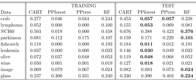
Table 3.3 Comparison of PPtree, CART, RF and PPF results with various data sets. The mean of training and test error rates from 200 re-samples is shown. (Order of rows is same as in Table3.2.) PPF performs favorably compared to the other methods. . . 30
Table 5.1 Rules to define the split value, c, between two groups, on a data pro-jection, using means, weighted mean, medians, standard deviations, in-terquartile ranges. . . 60
Table .1 Summary of functions implemented inPPforest. . . 73
Table .2 Summary of data included inPPforest package. . . 76
Table .3 Summary of available arguments of functionPPforest. . . 77
Table .4 Summary of available values of functionPPforest. . . 80
Table .5 Summary of available arguments of functionbaggtree. . . 81
Table .6 Summary of available arguments of functionnode data . . . 82
Table .7 Summary of available arguments of functionnode data . . . 83
Table .8 Summary of available arguments of functionPPtree split. . . 86
Table .9 Summary of output values of function PPtree split. . . 87
Table .10 Summary of available arguments of functionPPclassify2. . . 89
Table .11 Summary of available arguments of functiontrees pred. . . 89
LIST OF FIGURES
Figure 2.1 Classification tree model example with simulated data. In the left panel, a decision tree with six terminal nodes and 5 splits are shown. The right panel shows a scatterplot with the simulated data and the partition of
R2 into six regions corresponding to the six terminal nodes. . . 7
Figure 2.2 Projection pursuit classification tree model example with simulated data. In the left panel a decision tree with tree terminal nodes and 2 splits is shown. Right panel shows a scatterplot with the simulated data and the partition ofR2 into six regions corresponding to the three terminal
nodes. . . 10
Figure 3.1 Comparison of decision boundaries for therpart(left) andPPtree(right) algorithms on 2D simulated data. The partitions generated by PPtree algorithm are oblique to the axis, incorporating the association between the two variables. . . 18
Figure 3.2 Illustration of the PPtree algorithm for three classes. . . 20
Figure 3.3 Illustration of the PPforest algorithm. . . 23
Figure 3.4 Running time in seconds prior and post optimization for different pa-rameter options. . . 24
Figure 3.5 Illustration of simulation design. . . 28
Figure 3.6 Simulation results comparing efficiency of PPF relative to RF, for a range of correlations and variance. PPF almost always beats RF, and the efficiency increases as the angle defining the separation approaches 45o, and as σ (overlap between groups) increases. . . 29
Figure 3.7 Benchmark data results shown graphically. PPF performs consistently well across most of the data sets. . . 31
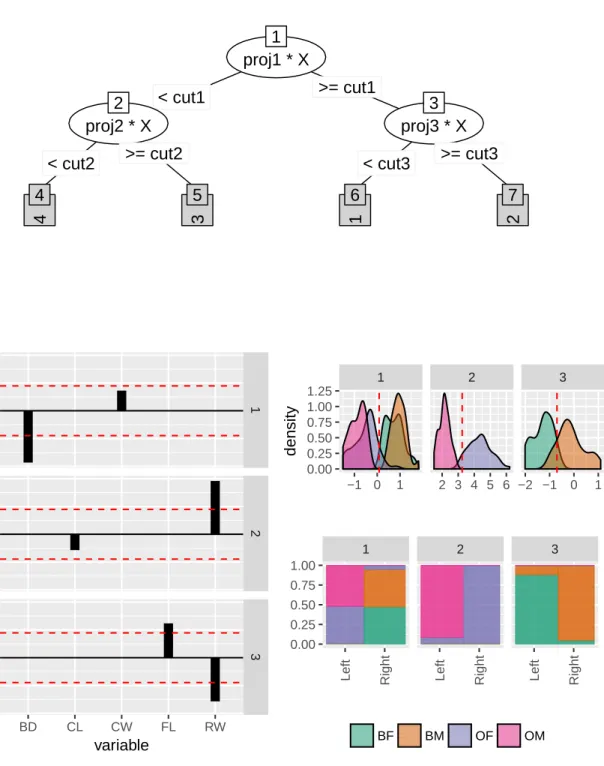
Figure 4.1 Visualizing the PPtree model of the crab data. The tree has three nodes (top). The density plots show the data projections at each node, colored by group (middle). The dashed vertical red line indicates the split value of each node. At node 1 the blue species is separated from orange species. Nodes 2 and 3 separate the sexes, which are more confused for the blue species. Mosaic plots of the confusion table for each split (bottom). Node 1 shows the clear split of the species, with a small number of misclassifications. Node 2 where orange females are separated from orange males indicates small number of misclassifications. Node 3 where blue females are separated from blue males, shows a larger misclassification than for orange specie. . . 38
Figure 4.2 Visualising the variable importance of all the trees in the forest, for three nodes. Each node of each tree has an importance value for each variable. The values for the whole forest are displayed using a side-by-side jittered dot plot. The importance values are the absolute values of the projection coefficients. The red points correspond to these values for the tree shown in Figure 2.2. Two variables are randomly selected at each node for creating the best projection, and split. The plots are right show the variables used and the split made at each of the nodes of this tree. . . 40
Figure 4.3 Examining similarity between cases, using pairwise plots of multidimen-sional scaling into 3D. It can be seen that most cases are grouped closely with their class, and particularly that the two species are distinct. There is more confusion of cases between the sexes. . . 41
Figure 4.4 Generalized ternary plot ((G-1)-D simplex, here it is a tetrahedron) representation of the vote matrix for four classes. The tetrahedron is shown pairwise. Each point corresponds to one observation and color is the true class. This is close but not a perfect classification, since the colors are concentrated in the corners and there are some mixed colors in each corner. . . 42
Figure 4.5 Another representation of the vote matrix, as a jittered side-by-side dotplot. It is not as elegant as the ternary plot, but it is useful because it places focus on each group. Each dotplot shows the proportion of times the case was predicted into the group, with 1 indicating that the case was always predicted to the group and 0 being never. On each dotplot, a single color dominates the top, indicating fairly clear distinctions between classes. Crabs from the blue species, both male and female, have more uncertainty in predictions, as seen by more crabs from other classes having higher vote proportions, than is seen in the orange species. . . 43
Figure 4.6 Entry page for the web app, focusing on examining cases, in terms of similarity and uncertainty. The top plot shows the data, the remaining plots show similarity of cases and uncertainty in predictions. All of the plots are linked, so that selecting elements of one will generate changes in the others. . . 46
Figure 4.7 Schematic diagram illustrating the interactivity in and between plots for individual level exploration panel of the web app. From the data, the four plots are generated. Each plot has a listener attached which collects user actions. When a user selects a point or line in any of the displays, it makes a change in the data which propagates updates to each of the plots. . . 47
Figure 4.8 The individual model tab in the web app. Variable importance is dis-played as jittered dot plots for three nodes of all trees. This is linked to a display of the PPTree, a boxplot of the error for all trees in the forest, and display of the data showing splits at each of three nodes and confusion tables as mosaic plots. Clicking a point in the jittered dotplot triggers various updates: each of the importance values for the same tree are highlighted (red), the tree that this corresponds to is drawn, the error for the tree is shown on the boxplot (in red), and the data displays are updated to show the tree. . . 49
Figure 4.9 Schematic diagram illustrating the interactivity in and between plots for model level exploration panel of the web app. Only the dotplot of variable importance is has click selection, which invokes changes of the tree display, boxplot, density plots and mosaic plots. Selecting a point, makes a change in the data, which propagates the importance values for other variables in this tree to be highlighted (red), draws the tree, highlights the error value of the tree, and shows the projections and confusion matrix for the three top nodes. . . 50
Figure 4.10 Performance comparison tab of the web app. ROC curves displaying sensitivity against specificity for the classes are shown, along with the OOB error by number of trees used to build the forest, and overall variable importance. Displays are shown for the PPF and RF, for com-parison purposes. Users can select a class to focus on, using the text entry box. . . 51
Figure 5.1 Illustration of the original PPtree algorithm for three classes. . . 58
Figure 5.2 Comparison of decision boundaries for therpart(left) andPPtree(right) algorithms on 2D simulated data. The partitions generated by PPtree algorithm are oblique to the axis, incorporating the association between the two variables. . . 59
Figure 5.3 Comparison of decision boundaries for therpart(left) andPPtree(right) algorithms on 2D simulated data. The partitions generated by PPtree algorithm are oblique to the axis, incorporating the association between the two variables. . . 59
Figure 5.4 Illustration of the algorithm using modification 1, for the three class problem. In each node in the second 1−D projection uses only infor-mation from the closest groups to find the best projection, and split. . 62
Figure 5.5 Illustration of the algorithm using modification 3, for the three classe problem. Projections of the data are still used at each node. Multiple steps for each class are allowed, and an impurity metric like entropy is used to determine when and how often to split cases in a node. . . 64
Figure 5.6 Model fits for the three different algorithms, rpart, PPtree and modified PPtree, on basic simulated data. For PPtree, rule 2 is used to determine the split values. The modified PPtree produces boundaries that are more symmetrically placed between clusters. . . 65
Figure 5.7 Model fits for the three different algorithms, rpart, PPtree and modified PPtree, for data where one class has two clusters. The boundaries induced by the multiple split PPtree reflect the shape of the data better than the other methods. . . 66
Figure 5.8 Boundaries induced by the three different algorithms for data simulated using a Gaussian mixture model. . . 67
Figure .1 Scatter plot matrix for crab data . . . 75
Figure .2 Visualizing the PPtree model of the crab data. The tree has three nodes (top). The density plots show the data projections at each node, colored by group (middle). The dashed vertical red line indicates the split value of each node. At node 1 the blue species is separated from orange species. Nodes 2 and 3 separate the sexes, which are more confused for the blue species. . . 84
Figure .3 Mosaic plots of the confusion table for each split. Node 1 shows the clear split of the species, with a small number of misclassifications. Node 2 where orange females are separated from orange males indicates small number of misclassifications. Node 3 where blue females are separated from blue males, shows a larger misclassification than for orange specie. 85
Figure .4 Tree structure plot usingPPtreeViz. . . 88
Figure .5 Generalized ternary plot ((G-1)-D simplex, here it is a tetrahedron) representation of the vote matrix for four classes. The tetrahedron is shown pairwise. Each point corresponds to one observation and color is the true class. This is close but not a perfect classification, since the colors are concentrated in the corners and there are some mixed colors in each corner. . . 92
ACKNOWLEDGEMENTS
I would like to thank, Di for all the patience, valuable guidance and support throughout these years. I love your courses, you are really passionate, creative and skillful to engage students.
I would like to thank, Heike for all your comments and to help me when I need it. I have enjoyed and learned a lot working with you in stat 528. I love how you always find interesting and creative problems for the class.
I am also grateful to Annette because she was an important part in my ISU experience. I have been working with her since my second semester at ISU. I have learned a lot about systematic review and meta-analysis, this topic is not part of this dissertation but will be part of my academic life.
I really appreciate the valuable comments and suggestions made by Dr. Eun-Kyung Lee that helped to improve the quality of my research work.
I would like to have something more than “thank you” for Nacho, to believe always in me more than anybody and to be part of my life. Thank you to take the risk in this incredible Ph.D. adventure, his constant support and also his valuable comments in my dissertation.
Nevertheless, I am also grateful to Alicia for be an important part of this Ph.D. experience, without your support this Ph.D. adventure would not have been possible
Finally, I would like to thank you to all my ISU friends because without them my ISU experience would be not as colorful as it was and special thank you to Nehemias for checking my writing when I need it.
ABSTRACT
Classification methods are widely used for types problems where rules to sort observations into groups are needed. There are many different methods to fit classification models but nothing is universally best. This research develops new classification methods, and visual tools for exploring the algorithms and results introduced in this work. The new classification method is a random forest built on trees using linear combinations of variables, which improves the predictive performance when the separation between classes is in combinations of variables. It is called a projection pursuit random forest (PPF). The benefit of the method is demonstrated using a simulation study, and on a suite of benchmark data. It is implemented in the R package, PPforest, with core functions in Rcpp to improve the computational speed. The process of bagging and combining results from multiple trees produces numerous diagnostics which, with interactive graphics, can provide a lot of insight into the class structure in high dimensions. A web app is designed and developed for this purpose. In the process of developing the PPF some deficiencies were observed in the tree algorithm, PPtree, forming the basic building block. This led to modifications to the algorithm, implemented in the R package, PPtreeExt, and a small web app to help digest differences between various model parameter choices.
CHAPTER 1. INTRODUCTION
This research develops new classification methods and visual tools for exploring the algo-rithms and results for classification problems. Algoalgo-rithms, like classification and regression trees (CART), are unstable because the model can vary substantially from one sample to an-other. Using bootstrap aggregated trees provides a more reliable classifier and one that better predicts new data. In Breiman (2001) two random forest methods were presented, one with trees calculated using axis-parallel partitions and other using trees with oblique partitions at random orientations. The second approach was not as successful as the first because it simply uses arbitrary projections. The space of projections is very big, so the RF rarely is capable of finding good oblique projections. However, interest in this approach has peaked in recent years. The new method presented in this dissertation is closer to the second original idea since it is a random forest built on trees using linear combinations of variables. This approach improves the predictive performance when the separation between classes is in combinations of variables. It is called projection pursuit random forest (PPF)
The trees used in the proposed ensemble, find the best split using a linear combination of variables instead of only one variable for each split. The main difference with the second random forest approach is that the oblique partitions are not selected at random, the linear combination is computed by optimizing a projection pursuit index, to get a projection of the variables that best separates the classes. Utilizing linear combinations of variables to separate classes takes the correlation between variables into account, and can outperform the basic forest when separations between groups occur on combinations of variables.
The benefit of the method is demonstrated using a simulation study and on a suite of benchmark data. It is implemented in the R package, PPforest, with core functions in Rcpp to improve the computational speed.
Statistical graphics are important in exploratory data analysis, model checking, and diag-nosis. There has been some, but not a lot of, research on visualizing classification models. The process of bagging and combining results from multiple trees produces numerous diagnostics which, with interactive graphics, can provide a lot of insight into the class structure in high dimensions. In this dissertation, a web app is designed to explore and diagnostic ensemble models and individual classifiers.
The visualization approach is consistent with the framework in Wickham et al. (2015a), and the implementation is built on the newest interactive graphics available in R. The purpose is to provide readily available tools for users to explore and improve ensemble fits and obtain an intuition for the underlying class structure in data. Interactive plots are a key component for model visualization that helps the user see multivariate relationships and be more efficient in the model diagnosis. Multiple levels of data are constructed for exploration: observation, model and ensemble summaries. The develop ideas are applied to the random forest algorithm, and to the projection pursuit forest, but could be more broadly applied to other bagged ensembles. In the process of developing the PPF, some deficiencies were observed in the tree algorithm, PPtree, forming the basic building block. This led to extensions to the projection pursuit tree (PPtree) algorithm for classification problems to enhance its performance in multi-class problems and in the presence of nonlinear separations. These extensions are implemented in the R package,PPtreeExt, and an interactive web app is also provided to explore the operation of the PPtree classifier and modifications under different scenarios.
The dissertation consists of four parts, including three independent papers and a user manual for PPforest package. Chapter 3 presents the proposed method, projection pursuit forest algorithm for supervised classification. The methodology is based on the previous work of Lee et al. (2013). The method is implemented in a new R package, called PPforest, available on GitHub. The algorithm incorporates methods to determine OOB error, variable importance, and proximity measures.
Chapter 4presents interactive graphics for visually diagnosing forest classifiers in R. Meth-ods to explore and diagnostic PPforest object. The visualization method can be used by other ensemble methods. In Chapter 5 modifications to the original PPtree algorithm are proposed
to improve the predictive performance of the algorithm and develop a more flexible tree struc-ture presents new modifications for the original projection pursuit tree algorithm. PPtreeExt is the R package which implements the new modifications. Appendix describes the software package that implements the projection pursuit forest for supervised classification method and documents usage with example code.
CHAPTER 2. LITERATURE REVIEW
Supervised and unsupervised learning are two important methods in statistical learning. The main objective of supervised learning is to predict the value of a response variableY for a given set of predictor variablesXT = (X1, . . . Xp). On the other hand, in unsupervised learning,
there is not information about the response variableY and the idea is to make inference about the density using only information from the predictor variables. When the objective is to predict a categorical variable then the supervised learning method is called classification problem while it is a regression problem when a quantitative outcome is predicted.
Classification problems can be addressed in different ways; we can use linear methods like linear regression, discriminant analysis, separating hyperplanes, etc. Additional approaches maybe based on kernel-smoothing methods, like kernel density estimation, mixture models for classification, etc. This project is focused on classification problems using bagged trees methods. In the next subsections, a literature review in trees and random forest is presented.
2.1 Classification and regression trees
Classification and regression trees are two supervised learning methods that have been used for a long time to solve a wide variety of problems. Classification trees are used when the objective is to predict a qualitative variable while is called regression when a quantitative outcome is predicted. These two techniques are not new, the first regression tree algorithm was published in 1963 (Morgan and Sonquist (1963)). Automatic Interaction Detection (AID) is the name of this regression tree algorithm.
After AID many other tree algorithms were developed across the years, CART Breiman et al. (1984), CHAID Kass (1980), C4.5 Quinlan (1993), FACT Loh and Vanichsetakul (1988),
QUEST Loh and Shih (1997), CRUISE Kim and Loh (2001), GUIDE Loh (2009), CTREE Hothorn et al. (2006) and many more. One key point differentiate some of these methods is the node spliting. Some of the methods use kernel density, nearest neighbor or linear splits on subset of variables in the node partition.
Decision trees can be grouped based on the number of predictor variables used in each node partition. Trees that use one variable at a node partition produce axis-parallel splits. While trees that test multiple feature variables at every node can produce oblique splits and are characterized to be smaller than axis-parallel ones.
One of the main attractive of classification trees is the simplicity to get the predictions. The most extended trees use binary partitioning with axis-parallel splits, like CART. These kinds of trees use only one variable in each split and then define hyperplanes that are orthogonal to the axis. In this thesis we will work with classification trees which define hyperplanes that are oblique to the axis. More specifically, projection pursuit classification tress (PPtree) algorithm will be used and these trees will be the base learner for a random forest approach.
2.1.1 Tree model
A tree can be seen as a set of decisions rules that define recursive partitions of the feature space. The expected values for the response variableY can be defined as follows:
E(Y /X =x) =
S X
s=1
csIRs(x) (2.1)
Where Rs represents a partition in the feature space such that Rs ∈R, with R =∪Si=1Ri
and the intersection of two partitions in R are exclusive, Rs ∩Ri = ∅. If x ∈ Rs then the
predicted value forY iscs.
IRs(x) = 1 if x∈Rs 0 if x /∈Rs
cs is computed differently if the problem is a classification or a regression problem.
For classification problems,Yi ∈ {1,2. . . K}denotes the class of each observation. Here the
cs= arg max k #(Y =k) #Rs Xi∈Rs
For regression problem the predicted value is :
cs= 1 #Rs X i/Xi∈Rs Yi
Finally for a given data set {Yi, X1i,X2i. . . Xpi}ni=1 the predicted values for the response
variable Y can be defined as ˆf(x) =PS
s=1ˆcsIRˆs(x) One thing that distinguish a single decision
tree algorithm is the way that the regions,Rs, are estimated.
2.1.2 Axis-parallel trees, CART
For axis parallel trees CART will be described. Classification and regression tress (CART) Breiman et al. (1984) is an important algorithm because was the first decision tree described with analytically rigor.
Given a training data of the form Θ = (X, Y), where Y is the response variables and
XT = (X
1, . . . Xp) the predictor variables. The main objective in CART is to predict the
values of the response using the information from X. The response and the feature variable can be quantitative or categorical variables. In a classification problem Y ∈ {1,2, . . . K} and the objective is to classify subjects in some of theK classes using information from the feature variables. If the response Y ∈ R is quantitative variable then CART has the same objective than a linear model, is to predict the numerical value of Y.
The CART decision tree produces binary recursive partitioning procedure by considering axis-parallel splits. This method split the feature space in rectangles using only one feature variable in each node split. Growing a tree beginning from a root node and split the data into two children subnodes. The main idea of node splitting is to get each child as pure as possible based on some impurity measure. Each children node is split again and this process stop when every distinct observation is in the training set has its own rectangle.
Figure2.1shows an example of classification tree with three classes and two feature variables base on simulated data. Data are simulated from three bivariate normal distribution with
| X1 < −2.54 X2 < −2.455 X2 < −2.865 X1 < 1.685 X1 < 1.465 sim1
sim3 sim2 sim3
sim2 sim3 −7.5 −5.0 −2.5 0.0 −5 0 5 X1 X2 Class sim1 sim2 sim3
Figure 2.1 Classification tree model example with simulated data. In the left panel, a deci-sion tree with six terminal nodes and 5 splits are shown. The right panel shows a scatterplot with the simulated data and the partition of R2 into six regions
corresponding to the six terminal nodes.
the following variance-covarance structure with ρ1 = 0.2, ρ2 = −0.35 and ρ3 = 0.25: Σi = 1 ρi ρi 1
, and different meanµ1= −5 −0.8 ,µ2= 3 2 and µ3 = 0 −4 .
In the tree diagram, we can see the values where the node was split and the order of the different partitions. In the first split X1 was used, and if and observation has X1 < −2.54
follow the left branch and otherwise follows the right branch. In the second partitionX2 was
used and a similar procedure was applied. In this example, six terminal nodes were defined and the regions associated to them were:
R1 = {X1 < −2.54}, R2 = {X1 ≥ −2.54, X2 < −2.865}, R3 = {−2.54 ≤ X1 <
1.685,−2.865 ≤ X2 < −2.4}, R4 = {X1 ≥ 1.685,−2.865 ≤ X2 < −2.4}, R5 = {X1 ≥
2.1.3 Tree construction
The construction of the optimal tree needs two basic steps. First, a ”maximal tree” is grown using the training data Θ = (X, Y). A set of partitions are used and in a simple way these partitions can be thought as a set of questions with binary response. x ∈ Q? where Q is a subset of the sample and the partition is created based on one variable. If Xi is a continuous
variables the test will have the form Xi < c vs Xi ≥c for some constantc ∈R, in case Xi is
categorical the test rule will be define asXi∈H vsXi∈/ H for some subsetH ⊂ {h1. . . h|Xi|} of the factors ofXi. For these two options in each node the test rule is checked and if the rule
is true (Xi < c or Xi ∈ H) the brunch follows to the left and if the condition is false the
brunch follows the right side.
All the partitions are evaluated and the best partition is selected based on some impurity measure of the node. The total number of possible splits when the predictor variable is cate-gorical withK categories is 2K−1−1 while ifXis continuous or ordinal withLdifferent values,
L−1 splits on X can be defined. After the best partition is selected, the initial data set is divided in two subsets and within each subset the same procedure is repeated. The second step consists in pruning the maximal tree to get the optimal tree. Instead of using a stopping rule the tree grows as large as possible and then the tree is pruned back to the root based on the lowest cross-validation estimation error which defines the place where the tree is pruned. Basically the next split to be pruned is the node which has the smaller contribution in the overall tree performance.
2.1.4 Impurity measures
For every nodeta set of decision rules are defined and the best rulesis selected using a node impurity measureI(t). This impurity measure of a node is associated with the heterogeneity of the dependent variable in this node. The way in which the heterogeneity is measure depends if the tree is a classification tree or a regression tree. In the first case, we have to take into account the characteristics of the qualitative variable while in the regression type the heterogeneity is given by the distribution of the continuous variable. For each rule s is defined φ(s, t) =
I(t)−I(tr)−I(tl) which represents the impurity reduction when a rule s is used to divided t. Finally the selected rule is the rule which maximizes φ(s, t), this is s∗ = arg maxs{φ(s, t)}. The optimization is done considering all the variables,s∗ is the best partition from all possible partitions.
2.1.5 Advantages & disadvantages
Some of the advantages we can mention about CART are the variable selection can be done automatically and the importance measure is given in a natural way. Quantitative and categorical variables can be used as dependent and independent variables. Are invariant to monotone transformations of the quantitative variables. Works with missing data. It is easy to interpret and fast to implement. One disadvantage is that these trees are unstable, also the there are some works that show the induction of bias in the variable selection. Finally, these trees make the separation only using one variable in each node partition then does not work well when the data can be separable with linear combinations.
2.2 Oblique splits trees, PPtree
One of the limitations of trees like CART is that the nodes can only separate the data with hyperplanes orthogonal to the feature axis. Oblique trees uses discriminant functions in each node with more than one variable, then the defined hyperplanes are oblique to the axes (polygonal partitioning of the feature space). Oblique trees tend to be more interpretable than axis-parallel trees. Two kinds of oblique trees can be defined based if they use all the feature variables or only some of them, then full or concise oblique trees can be defined.
To describe oblique split trees I will focus on projection pursuit classification tree (PPtree) Lee et al. (2013), these trees are of interest in this oblique trees review because they are the basic learning of the bagging classification method purposed in this work. PPtree optimize a projection pursuit index to find low-dimensional projections to separate classes.
PPtree method is defined for classification problems where the response variable is categor-ical and the method is define to use quantitative feature variables.
Projection Pursuit Classification Tree proj1 * X1 < cut1 >= cut1 sim1 2 proj2 * X 3 < cut2 >= cut2 sim2 4 sim3 5 −5.0 −2.5 0.0 −5 0 5 X1 X2 Class sim1 sim2 sim3
Figure 2.2 Projection pursuit classification tree model example with simulated data. In the left panel a decision tree with tree terminal nodes and 2 splits is shown. Right panel shows a scatterplot with the simulated data and the partition ofR2 into six
regions corresponding to the three terminal nodes.
One important characteristic of PPtree is that treats the data always as a two-class system when the classes are more than two the algorithm uses a two-step projection pursuits opti-mization in every node split. In the first step optimize a projection pursuit index to redefine the problem in a two class problem and the second step is to find an optimal one-dimensional projection to separate the two class problem. Base on this process to grow the tree, the depth of PPtree is at most the number of classes. PPtree uses binary partitioning test, if Xi is a
continuous variables the test will have the form Pp
i=1αiXi < c vs Pp
i=1αiXi ≥ c for some
constantc∈Rand the coefficientsαi∈R. In each node, the test rule is checked and if the rule
is true (Pp
i=1αiXi < c) the brunch follows to the left and if the condition is false the brunch
follows the right side. Figure2.2shows an example of classification projection pursuit tree with three classes and two feature variables base on the same simulated data described before.
In this simple example the two feature variables are linearly combined to do the partitions en each split. In the first split if an observation has 0.91X1 + 0.40X2 < −2.90 follow the
left branch and if no, follow the right branch. In the second partition if an observation has 0.46X1−0.88X2 < 2.61 follows the left branch and if no, follows the right branch. In this
R1 = {0.91X1 + 0.40X2 <−2.90}, R2 = {0.91X1+ 0.40X2 ≥ −2.90,0.46X1−0.88X2 <
2.61},and R3={0.91X1+ 0.40X2 ≥ −2.90,0.46X1−0.88X2 ≥2.61}
2.2.1 Tree construction
Using the training data Θ = (X, Y) a full (maximal) tree is grown. As in CART, we can think in the partitions as a set of questions with a binary response. x∈Q? whereQis a subset of the sample and the partition is created based on one a linear combination of variables. In the PPtree construction, the data are treated always as a two-class system, when the classes are more than two the algorithm uses a two-step projection pursuits optimization in every node split. In the first step, an optimal one-dimension projection α∗ is found, for separating all classes in the current data. All the data are projected inα∗ and comparing means the classes are reduced to two classes. A new variable y∗i is defined by assigning a new label “G1” or “G2” to each observation. The new groups “G1” and “G2” can contain more than one original classes. Then a second projection pursuit optimization is done using these new group labels,
G1 andG2, to finding the optimal one dimension projection, α, using (Xi, yi∗). This step is to
find the best separation between “G1” and “G2”, if Pp
i=1αiM1< c then assign “G1” to the
left node else assign “G2” to the right node, where M1 is the mean of “G1”. This procedure is repeated for each node until there is one class in each node from the original classes.
2.2.2 Impurity measure
Let (p1, p2. . . pK) the probabilities for each class in the training data. LetZi=αTXi where αis a p-dimensional projection in a 1-dimensional space. The projected data were examined in two ordered groups Z(1). . . Z(i) and Z(i+1). . . Z(n) , and the class probabilities for each group were defined for a given i like (pLi,1. . . pLi,g) and (pRi,1. . . pRi,g) where and pLi and pRi be the proportion of each group. To measure the impurity of each group the class probability measure was used and IMLi (impurity measure for left group) and IMRi (impurity measure for right) can be calculated. To find the best split i∗ for the projected data {Z(1). . . Z(i∗)}
and {Z(i∗+1). . . Z(n)} we have to minimized the weighted mean of the impurity measures,
IMi =pLiIMLi+pRiIMRi and get IM
∗
partitions are evaluated and the best partition is selected based on the impurity measureIMi
(Lee et al., 2005).
2.2.3 Advantages & disadvantages
PPtree has a simpler structure than other tree methods like CART. The number of classes will be the same as the number of final nodes, so the depth of the tree is at mostK−1 where
K is the number of classes. PPtree does not need to be pruned as CART does. In PPtree the correlation between the original variables is taken into account in the tree construction. At each node, the PPtree separates two classes using a linear combination andif a linear boundary exists
in the data, PPtree produces a tree without misclassification. Another interesting characteristic is this method can be used for variable selection since each projection coefficient of each node represents the importance variable to separate classes in each node.
2.3 Random forest
A random forest is an ensemble learning method, built on bagged trees developed by Breiman (2001). There are two main concept used in random forest, bootstrap aggregation (Breiman (1996) and Breiman et al. (1996)) and random feature selection (Amit and Geman (1997) and Ho (1998)) to individual classification or regression trees for prediction. Bootstrap samples from training test and random feature selection in each split are the two ways in which random forest incorporate randomness in the model. The most used random forest implemen-tation uses CART or C4.5 trees as individual learners, these trees generate partitions that use only one feature variable generating boundaries with box structure.
Let Θ = (X, Y) the training set of size N,B bootstrap samples with size N are extracted. For each bootstrap sample, a tree is grown using random variable selection in each node and the trees are not pruned. In this process as in bagging the variance is reduced due to the aggregation and the bias because the trees are fully grown. Additionally, to bagging the trees correlation in the random forest is reduced because of the random feature selection in each split. The number of selected variables to use in each node split should be much smaller than the total number of variables. In the case of classification they recommendp(m) in classification
problems and m3 in regression problems. In each node, the best split based on the selected variables is done. Final predictions are obtained by aggregating the results from the trees if the problem is classification the final result is based on majority vote while if the problem is regression the prediction is base on average over the trees. A formal definition of random forest from Breiman (2001) is:
Definition: A random forest is a classifier consisting of a collection of tree-structured classi-fiers {h(x,Θk), k= 1, . . .} where {Θk} are independent, identically distributed random vectors
and each tree cast a unit vote for the most popular class at input x.
Where Θk is a random vector where each Θk is independent from Θ1, . . . ,Θk−1 but with
the same distribution. h(x,Θk) is a single decision tree. The random forest error rate depends
on the correlation between the trees in the forest and the strength of each individual tree in the forest (Breiman, 2001). The expected values for the response variable Y in random forest can be defined as follows:
For classification E(Y /X =x) = arg max k B X b=1 I[Eb(Y /X =x) =k] (2.2) For regression E(Y /X =x) = 1 B B X b=1 Eb(Y /X =x) (2.3) 2.4 Model visualization
A conceptual framework for model visualization can be summarized in three strategies: (1) visualize the model in the data space, (2) look all members of a collection of a model and (3) explore the complete process of model fitting (Wickham et al., 2015a). The first strategy is to explore how well the model captures the data characteristics (model in the data space), which contrasts determining if the model assumptions hold (data in the model space). The second strategy is to look at a group of models instead of only the best. This strategy can offer a broad understanding of the problem by comparing and contrasting possible models. The last strategy focuses on the exploration of the process of the model fit in addition to the end result.
There has been some, but not a lot of, research on visualizing classification models. Urbanek (2008) presents interactive tree visualization implemented in the Java software called KLIMT
that include zooming, selection, multiple views, interactive pruning and tree construction as well as the interactive analysis of forests of trees using treemaps. Cutler and Breiman (2011) developed a Java package called RAFT to visualize a forest classifier, that included variable selection, parallel coordinate plots, heat maps and scatter plots of some diagnostics. Linking between plots is limited. Quach (2012) presents interactive forest visualization using the R package iPlots eXtreme (Urbanek, 2011), where several displays are shown in the one win-dow with some linking between them available. Silva and Ribeiro (2016) describes visualizing components of an ensemble classifier.
CHAPTER 3. A PROJECTION PURSUIT FOREST ALGORITHM FOR SUPERVISED CLASSIFICATION
Abstract
A random forest is an ensemble learning method built on bagged trees with random pre-dictor selection. These feature provide improved classification models because they produce information about the variable importance, predictive error, and proximity of observations. This paper presents a new ensemble learning method for classification problems called projec-tion pursuit random forest (PPF). PPF uses the PPtree algorithm introduced in Lee et al. (2013).
In PPF, trees are constructed by splitting on linear combinations of randomly chosen vari-ables. Projection pursuit is used to choose a projection of the variables that best separate the classes. Utilizing linear combinations of variables to separate classes takes the correla-tion between variables into account which allows PPF to outperform the tradicorrela-tional random forest when separations between groups occur in combinations of variables. Previous work using oblique trees in the forest construction have shown positive results in terms of per-formance but are only for two-class problems. The method presented here can be used in multi-class problems and is implemented into an R package, PPforest, which is available at
3.1 Introduction
There are two main aspects of a random forest (Breiman, 2001), bootstrap aggregation and (Breiman, 1996; Breiman et al., 1996) random predictor selection(Amit and Geman, 1997; Ho, 1998). These aspects are broadly applicable to build ensemble classifiers from any basic method; bagging stabilizes the variance and random predictor selection reduces correlation between trees in the forest.
This paper presents the projection pursuit random forest (PPF), a new ensemble learning method for classification problems, which utilizes combinations of predictors in the tree con-struction. For each split, a random sample of predictors is selected, then an optimal linear combination for separating the classes is computed by using a projection pursuit index. The algorithm is targeted at problems where classes can be separated by linear combinations of predictors variables which define hyperplanes that are oblique to the axes rather than orthog-onal to them. Additiorthog-onally PPF accommodates class imbalance by using stratified bootstrap samples and variable importance measures can use the coefficients of the projections used in PPF.
Trees that use linear combinations of predictors in a split are known in the literature as oblique trees (Kim and Loh, 2001; Brodley and Utgoff, 1995; Tan and Dowe, 2005; Truong, 2009; Lee et al., 2013). All these trees look for linear combinations of predictors to use in a split, and the main difference between them is the method for selecting the linear combination. Some of the methods used for selecting the linear combination include random coefficient generation, penalized least squares, L2-regularization or linear support vector machines. It is important to note that most of the oblique trees methods are not available for use, or the code is not open source, e.g. Kim and Loh (2001).
Tan and Dowe (2006), Menze et al. (2011) and Do et al. (2010) present random forest algorithms that use oblique trees as the base. The research has shown positive results in terms of performance compared with other methods (CART, SVM, RF among others), but either the code is not available or they are limited to two-class problems.
PPF is built on thePPtreealgorithm (Lee et al., 2013) implemented in R which fits a single multi-class oblique tree to the data. Two projection pursuit indexes are available in PPF: LDA and PDA1. PPF can be used for multi-class problems and is implemented into an R package, calledPPforest.
The projection pursuit algorithm searches for a low dimensional projection that optimizes a continuous function which measures some aspect of interest; for PPF, this is class separa-tion. Friedman and Tukey (1973) coined the term “projection pursuit”, but the ideas existed earlier than this (Kruskal, 1969). Lee et al. (2005) developed an index, derived from the linear discriminant analysis, for finding projections that separate classes. Letxgi be a p-dimensional data vector, i-th observation of the g-th class, g = {1, . . . , G}, G is the number of classes,
i={1, . . . , ng}, andng is the number of observations in class g. The LDA index is defined as
follows: ILDA(A) = 1− | |ATW A| AT(W+B)A| for|AT(W +B)A| 6= 0 0 for|AT(W +B)A|= 0 (3.1) where B = PG
g=1ng(¯xg.−x¯..)(¯xg.−x¯..)T is the between-group sums of squares, and W = PG
g=1 Png
i=1(xig−¯xg.)(xig−x¯.g)T is the within-group sums of squares. If the LDA index value is high, there is a large difference between classes.
A second index, PDA, was developed to address large p, small n data (Lee and Cook, 2010). The main idea used in construction of the index is that when n ≤ p or the variables are highly correlated, the maximum likelihood variance-covariance matrix estimator will be close to being singular, and this will affect the inverse calculation. The PDA index adjusts the variance-covariance matrix calculation, and is defined as follows:
IP DA(A, λ) = 1−
|ATWP DAA|
|AT(W
P DA+B)A|
(3.2) where A is an orthonormal projection onto a k-dimensional space and λ ∈ [0,1) is a pre-determined parameter. B is the between-class sums of squares and WP DA = diag(W) + (1− λ)offdiag(W).
−4 −2 0 2 −4 −2 0 2 4 X1 X2 −4 −2 0 2 −4 −2 0 2 4 X1 X2
Figure 3.1 Comparison of decision boundaries for the rpart (left) and PPtree (right) algo-rithms on 2D simulated data. The partitions generated by PPtree algorithm are oblique to the axis, incorporating the association between the two variables.
The PPtree algorithm uses a multi-step approach to fit a multi-class model by finding linear combinations to split on. Figure 3.1 compares the boundaries that would result from a classification tree fitted using the rpart algorithm (Therneau et al., 2010) and the PPtree algorithm.
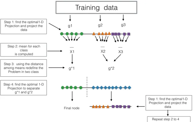
Figure 3.2 illustrates the PPtree algorithm for three classes, and the algorithm steps are detailed below. Let dn = {(xi, yi)}ni=1 be the data set where xi is a p-dimensional vector
of explanatory variables and yi ∈ G (G = {1,2, . . . G}) represents class information with i= 1, . . . n.
1. Optimize a projection pursuit index to find an optimal one-dimensional projection, α∗, for separating all classes in the current data yielding projected dataz=α∗x.
2. On the projected data, z, redefine the problem into a two class problem by comparing means, and assign a new label, eitherg∗1 org2∗to each observation, generating a new class variableyi∗. The new groups g∗1 and g∗2 can contain more than one original class.
3. Find an optimal one-dimensional projection α∗∗, using {(xi, yi∗)}n
i=1 to separate the two
class problem g∗1 and g∗2. The best separation of g1∗ and g2∗ is determined in this step providing the decision rule for the node,
ifα∗∗TM1 < cthen assign g∗1 to the left node else assign g2∗ to the right node,
whereM1 is the mean of g1∗.
4. For each group, all the previous steps are repeated until g1∗ and g∗2 have only one class from the original classes. The depth of PPtree is at most the number of classes.
This paper describes extending the PPtree into a PPforest and is organized as follows. Section 3.2 describes the PPF algorithm; diagnostics, including how to compute variable im-portance; and implementation details. Section 3.3 evaluates the algorithm using a simulation study and performance on benchmark machine learning data in comparison with other methods. Section3.4 discusses possible extensions and future directions.
3.2 Projection pursuit random forest
This section provides the definition of PPF for classification and the algorithm. Diagnostics for the classifier are also defined.
3.2.1 Definition
Let the random vector of predictor variables X ∈ Rp and the output random variable
Y ∈ G, where G is a finite set such that G = {1,2, . . . , G}. The training sample is defined asDn={(X1, Y1), . . .(Xn, Yn)} of i.i.d<p×G random variables (p≥2). The objective is to
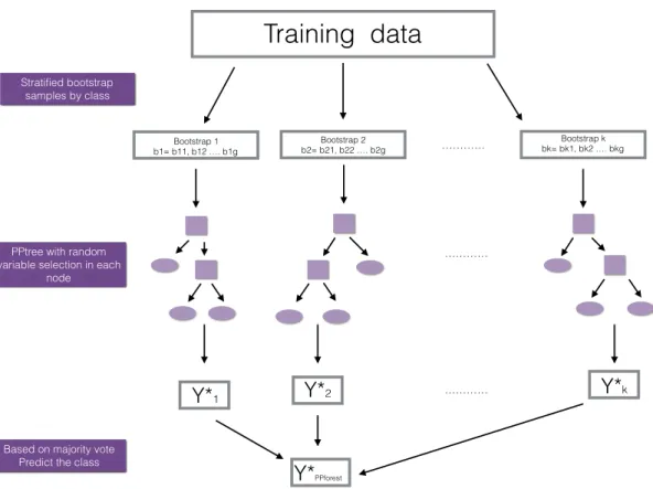
Stratified bootstrap samples by classStratified bootstrap samples by class bootstrap samples by class
Training data
Step 1: find the optimal1-DProjection and project the data — X1 — X2 — X3
Step 2: mean for each class is computed
g1 g2 g3
g*1 g*2
Step 3: using the distance among means redefine the
Problem in two class
Step 4: find the optimal 1-D Projection to separate
g*1 and g*2
Final node
Repeat step 2 to 4 Step 1: find the optimal1-D
Projection and project the data
Figure 3.2 Illustration of the PPtree algorithm for three classes.
A projection pursuit classification random forest can be defined as a collection of randomized classification trees{hn(x,Θm, Dn), m≥1}where{Θm}are i.i.d. random vectors. Θmincludes
the two sources of randomness in the tree (random variable selection and random bootstrap sample), then Θm has information about which variables were selected in each partition and
which cases were selected in the bootstrap sample.
For each tree, hn, a unique vote is collected based on the most popular class for the selected
predictor variables. Equation3.3defines the PPF estimator based on combining the trees.
fn(X, Dn) = arg max g∈G {EΘ(I[hn(X,Θ, Dn) =g])} (3.3) = arg max g∈G PΘ(hn(X,Θ, Dn) =g)
EΘ is the expectation wrt Θ, conditionally on X and Dn. In practice, the PPF estimator is
evaluated by generatingB random trees and take the average of the individual outcomes. This procedure is justified in a similar way to the original random forest defined by Breiman (2001), and is based on the Law of the Large Numbers (Athreya and Lahiri, 2006).
Equation 3.4describes the prediction of a new observation x0.
ˆ fn(x0) = arg max g∈G B X k=1 I[hn(x0,Θbk) =g] (3.4) 3.2.2 Algorithm 1. Letn=PG
i=1nithe total number of cases in the training setdn={xi, yi}ni=1. Bstratified
bootstrap samples from dn are taken. Then for each class, independently and uniformly
re-sample cases fromdng (training data set for groupg) with sizeng to create a stratified
bootstrap data set{bk=bk1, bk2, . . . bkg}.
2. Use a bootstrap sample bk to grow a PPtree (hn(x,Θbk)) to the largest extent possible
without pruning. (Note that the depth of the PPtree is at most G−1, where G is the number of classes).
(a) Start with all the cases inbk in the root node.
(b) A simple random sample of m predictor variables from the set of all the predictor variables M is drawn, where m << M.
(c) Find the optimal one-dimensional projectionα∗ to separate all the classes in bk.
(d) If more than two class, then reduce the number of classes to two by comparing means, and assign new labels,g∗1 andg∗2 to each case (called the new responseyi∗ in
bk).
(e) Find the optimal one-dimensional projection,α∗∗, using the bootstrap data set with the relabeled response, y∗, to separate g1∗ and g∗2. The linear combination is com-puted by optimizing a projection pursuit index to get a projection of the variables
that best separates the classes using the m random selected variables. Two index options are available LDA or PDA.
(f) Compute the decision boundaryc. Eight different rules to define the cutoff value of each node can be used.
(g) Keep α∗∗ and c.
(h) Separate the data into two groups using the new labelsg1∗ and g∗2. (i) Repeat from (b) to (h) if g1∗ org2∗ have more than two original classes.
3. Repeat 2 for k= 1, . . . B.
4. The output is the ensemble of PPtrees,{hbkn}B k=1.
Split values on the projected data can be computed by one of eight methods, which use the group means, or medians, sample size and variance or IQR weighting
Figure 3.3has a diagram illustrating the PPforest algorithm.
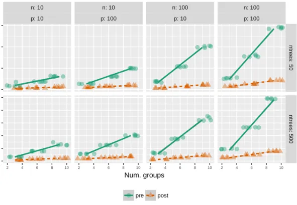
3.2.3 Implementation
The initial code for PPforest was developed entirely in R. It was subsequently profiled usingprofvis(Chang and Luraschi, 2016), and two code optimization strategies were employed: translate main functions into Rcpp (Eddelbuettel et al., 2011) and parallelization using plyr. The microbenchmark package was used to compare the speed before and after optimization. Figure3.4shows the performance before and after optimization. The decrease in speed is linear as the number of groups increases. The improvement is between 3- and 9-fold for this range of parameters. The machine used for this comparison was a MacBook Pro with a processor of 2.4 GHz Intel Core i7 with a memory of 8GB and 1867MHz LPDDR3.
Training data
Bootstrap 1 b1= b11, b12 …. b1g Bootstrap 2 b2= b21, b22 …. b2g Bootstrap k bk= bk1, bk2 …. bkg ………… Stratified bootstrap samples by classPPtree with random variable selection in each
node
Y*
1Y*
2Y*
kBased on majority vote Predict the class
Y*
PPforest…………
…………
Figure 3.3 Illustration of the PPforest algorithm.
3.2.4 PPF diagnostics
The process of bagging and combining results from multiple trees produces numerous diag-nostics which can provide a lot of insight into the class structure in high dimensions. Because ensemble methods are composed of many models fitted to subsets of the data, many statistics can be calculated to be analyzed as a separate data set. This provides the ability to understand how the model is working. The diagnostics of interest are the error rate, variable importance measure, vote matrix, and proximity matrix.
3.2.4.1 Error rate
Using the out-of-bag (oob) cases from bagged trees in the forest construction allows ongoing estimates of the generalization error for an ensemble of trees, described in Breiman (2001).
n: 10 p: 10 n: 10 p: 100 n: 100 p: 10 n: 100 p: 100 ntrees: 50 ntrees: 500 2 4 6 8 10 2 4 6 8 10 2 4 6 8 10 2 4 6 8 10 0 5 10 15 0 25 50 75 100 125 Num. groups Time (sec) pre post
Figure 3.4 Running time in seconds prior and post optimization for different parameter op-tions.
Table 3.1 Optimization assessment simulation design Parameters Values g= number of classes (3,32,33) n= obs. by class (101,102) p= number of variables (101,102) m= number of trees (50, 500) cr= numbers of cores (1,2,4)
v PPforest version (new, old)
Given a training data set dn, B bootstrap samples from dn are taken. For each bootstrap
sample (b = 1,2, . . . B), a PPtree classifier hn(x,Θb) is constructed, and a majority vote is
used to get the PPF predictor. The oob cases are used to get the error rate estimates. For each {xi, yi} in dn, the votes are aggregated only for the classifiers hn(x,Θb) that do not contain
{xi, yi}. Hence, PPF is called the out-of-bag classifier, and the error rate for this classifier
(out-of-bag error rate) is the estimate of the generalized error. The out-of-bag error rate is a measure for each model that is combined in the ensemble and is used to provide the overall error of the ensemble.
3.2.4.2 Variable importance
PPF calculates variable importance in two ways: (1) permuted importance using accuracy, and (2) importance based on projection coefficients on standardized variables. The permuted variable importance is comparable to the measure defined in the classical random forest algo-rithm. It is computed using the oob cases for the treek (B(k)) for eachXj predictor variable.
Then the permuted importance of the variable Xj in the treek can be defined as:
IM P(k)(Xj) = P
i∈B(k)I(yi = ˆyi(k))−I(yi = ˆyi,P(k)j)
|B(k)|
where ˆyi(k)is the predicted class for the observation i in the tree k, and yi,P(k)
j is the predicted class for the observationiin the tree k after permuting the values for variable Xj. The global
measure is based on comparing the accuracy of classifying oob observations using the true class with permuted (nonsense) class.
For the second importance measure, the coefficients of each projection are examined. The magnitude of these values indicates importance if the variables have been standardized. The variable importance for a single tree is computed by a weighted sum of the absolute values of the coefficients across node, then the weights take the number of classes in each node into account(clnd) (Lee et al., 2013) . The importance of the variable Xj in the PPtree k can be
defined as: IM Ppptree(k) (Xj) = nn X nd=1 |α(ndk)| clnd
where α(ndk) is the projected coefficient for node ns and variable k and nn the total number of node partitions in the treek.
The global variable importance in a PPforest then can be defined in different ways. The most intuitive are the average variable importance from each PPtree across all the trees in the forest. IM Pppf orest1(Xj) = PK k=1IM P (k) pptree(Xj) K
Alternatively, a global importance measure is defined for the forest as a weighted mean of the absolute value of the projection coefficients across all nodes in every tree. The weights are based on the projection pursuit indexes in each node (Ixnd), and 1-(OOB-error of each tree)(acck).
IM Pppf orest2(Xj) = PK k=1acck Pnn nd=1 Ixnd|α (k) nd| nn K 3.2.4.3 Proximity matrix
In a tree, each pair of observations can be in the same terminal node or not. Tallying this up across all trees in a forest gives the proximity matrix, an n×n matrix of the proportion of trees that the pair shares a terminal node. A proximity matrix can be considered to be a
similarity matrix. This is typically used to do a follow-up cluster analysis to assess the strength of the class structure, and whether there are additional unlabeled clusters.
3.2.4.4 Vote matrix
An uncertainty measure for each observation, across models, is the proportion of times that a case is predicted to be in each class. If a case is always predicted to be the one class, there is no uncertainty about its group, and if this matches the true class then it is correctly labeled. Cases that are proportionately predicted to be multiple classes indicate difficult-to-classify observations. These cases may be important in that they might indicate special attention is needed in some neighborhoods of the data space, or more simply, could be errors in measurements in the data.
3.2.4.5 Summary
These diagnostics are used to assess model complexity; individual model contributions; variable importance and dimension reduction; and uncertainty in prediction associated with individual observations. da Silva et al. (2017a) provides more details and describes structuring data and constructing plots to explore forest classification models interactively. Interactive graphics are built inR, using theggplot2,plotly, and shinypackages.
3.3 Performance comparison
This section presents simulation results and a benchmark data study to examine the pre-dictive performance of PPF in comparison to other methods. In the benchmark data study, PPF is compared with PPtree, CART and RF. The simulation results are designed to compare PPF with RF on data with linear projections defining class differences.
3.3.1 Simulation study
A simulation study is designed to understand the performance of PPF relative to that of RF, when the separation between classes is in linear combinations of variables. PPF should outperform RF. Two parameters are varied,σ, θ, in the design illustrated by Figure3.5.
𝜇
-
𝜇
𝜎
𝜃
𝜎
Figure 3.5 Illustration of simulation design.
Each 2D simulated data set was rotated from 0 through 45o, and 10 replications were conducted. Mean difference was fixed at 0.3, andσranged from 0.1-0.3, which is the proportion of the standard deviation in the orthogonal direction. The results are shown in Figure 3.6, PPF almost always beats RF, and the efficiency increases as the angle defining the separation approaches 45o, and as σ (overlap between groups) increases.
3.3.2 Benchmark data study
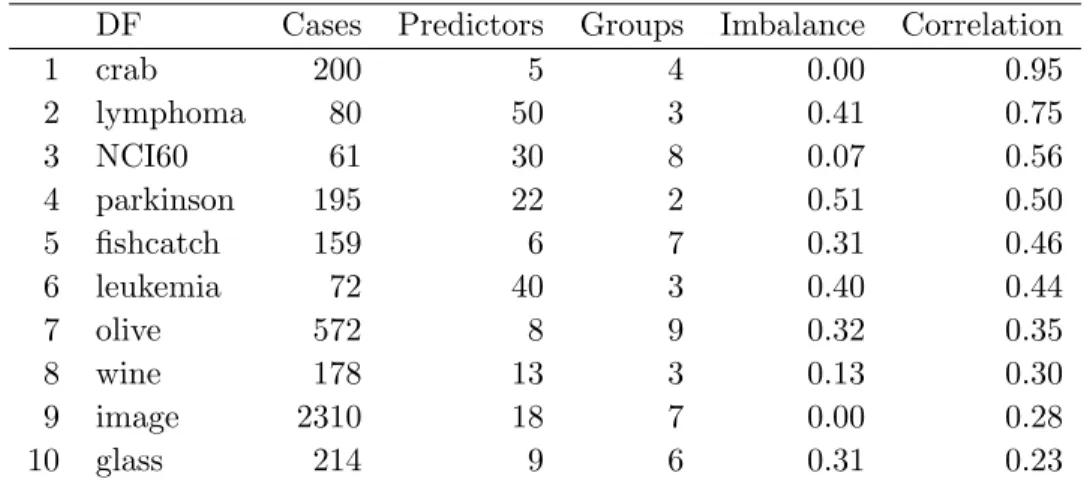
The performance of PPF is compared with the classification methods, PPtree, CART and RF using 10 benchmark data sets taken from the UCI Machine Learning archive (Lichman, 2013). Table3.2presents summary information about the benchmark data, number of groups, cases, and predictors for each data set. Theimbalance between groups is measured by the range
0.1 0.15 0.2 0.25 0.3 0.0 0.5 1.0 0.0 0.5 1.0 0.0 0.5 1.0 0.0 0.5 1.0 0.0 0.5 1.0 1.00 1.02 1.04 correlation efficiency
Figure 3.6 Simulation results comparing efficiency of PPF relative to RF, for a range of cor-relations and variance. PPF almost always beats RF, and the efficiency increases as the angle defining the separation approaches 45o, and as σ (overlap between groups) increases.
of group size proportions and correlation is the average of all pairwise correlation coefficients among predictor variables.
Table 3.2 Summary of benchmark data. Imbalance and correlation indicating relative class sizes, and separations in combinations of variables
DF Cases Predictors Groups Imbalance Correlation
1 crab 200 5 4 0.00 0.95 2 lymphoma 80 50 3 0.41 0.75 3 NCI60 61 30 8 0.07 0.56 4 parkinson 195 22 2 0.51 0.50 5 fishcatch 159 6 7 0.31 0.46 6 leukemia 72 40 3 0.40 0.44 7 olive 572 8 9 0.32 0.35 8 wine 178 13 3 0.13 0.30 9 image 2310 18 7 0.00 0.28 10 glass 214 9 6 0.31 0.23
For each benchmark data set, 2/3 of the observations are randomly chosen and used for training while the remaining 1/3 are used as test data for computing predictive error. This procedure is repeated 200 times and the mean error rate is reported in Table 3.1. In PPF, the number of variables selected in each node partition is a tuning parameter, the proportion of variables selected at each partition. Three different values were used (0.6, 0.9 and the RF default). The test error reported for PPF is the best from these. The results show that PPF has a better performance in the test data set than the other methods for the crab, fishcatch,
leukemia, lymphoma, olive and wine data, while the RF test error is smaller for glass, image, NCI60 and parkinson data.
Table 3.3 Comparison of PPtree, CART, RF and PPF results with various data sets. The mean of training and test error rates from 200 re-samples is shown. (Order of rows is same as in Table3.2.) PPF performs favorably compared to the other methods.
TRAINING TEST
Data CART PPforest PPtree RF CART PPforest PPtree RF crab 0.277 0.046 0.044 0.244 0.453 0.057 0.057 0.238 lymphoma 0.052 0.000 0.000 0.100 0.155 0.053 0.069 0.081 NCI60 0.503 0.019 0.000 0.458 0.676 0.388 0.423 0.376 parkinson 0.081 0.112 0.175 0.107 0.159 0.171 0.229 0.101 fishcatch 0.118 0.000 0.000 0.193 0.184 0.011 0.012 0.191 leukemia 0.037 0.000 0.000 0.033 0.146 0.030 0.049 0.032 olive 0.072 0.037 0.048 0.053 0.119 0.048 0.068 0.052 wine 0.050 0.001 0.001 0.019 0.127 0.018 0.021 0.021 image 0.069 0.079 0.067 0.024 0.082 0.083 0.073 0.024 glass 0.237 0.306 0.331 0.240 0.330 0.390 0.403 0.224
Figures3.7displays the performance comparison graphically. Each line connects the errors for one data set. Even though RF outperforms PPF on almost half the data (Table 3.1) PPF tends to have consistently low error.
3.4 Discussion
This article presents a new ensemble method (PPF) for classification problems, that utilizes linear combinations of variables to separate classes. PPF takes the correlation between variables into account and can outperform the random forest when separations between groups occur on combinations of variables.
PPF method combines both advantages of oblique node split and ensemble methods in a convenient way to improve the predictive performance, whilst maintaining the ability to understand the model.
In the benchmark data study presented in this paper, PPF performance is always better than CART and PPtree, and often better than RF. Simulation results show that PPF performs
Training Test ppf pptr rf cartppf pptr rf cart 0.0 0.2 0.4 0.6 Method A v er age error r ate Data crab fishcatch glass image leukemia lymphoma NCI60 olive parkinson wine
Figure 3.7 Benchmark data results shown graphically. PPF performs consistently well across most of the data sets.
better than RF when the classes are separated by a linear combination of variables and when the correlation between variables increases.
Two projection pursuit indexes, LDA and PDA, are available for PPF and more could be substituted. Different projection pursuit functions may extend of the PPtree and PPforest to tackle other types of data problems: a continuous rather than categorical response variable, or when there is no response variable and the purpose is to group observations to construct a class variable.
Lastly, the work on PPF has revealed some enhancements of the PPtree algorithm to get a better separation of classes more broadly. For example, in the current algorithm the boundaries of the model can be too close to some of the classes. Tweaking the classification step of the algorithm can fix this. Also, allowing the algorithm to continue splitting data beyond the number of classes, could help to tackle nonlinear classification problems.
3.5 Acknowledgements
The code for PPF are implemented in an R (R Core Team, 2016) package, PPforest, available onhttps://github.com/natydasilva/PPforest, to be submitted to CRAN http:
//cran.r-project.org.
This paper was written with the R packages knitr (Xie (2015)), ggplot2 (Wickham (2009)) and dplyr (Wickham et al. (2015b)).
CHAPTER 4. INTERACTIVE GRAPHICS FOR VISUALLY DIAGNOSING FOREST CLASSIFIERS IN R
Abstract
This paper describes structuring data and constructing plots to explore forest classification models interactively. A forest classifier is an example of an ensemble since it is produced by bagging multiple trees. The process of bagging and combining results from multiple trees produces numerous diagnostics which, with interactive graphics, can provide a lot of insight into class structure in high dimensions. Various aspects are explored in this paper, to assess model complexity, individual model contributions, variable importance and dimension reduction, and uncertainty in prediction associated with individual observations. The ideas are applied to the random forest algorithm and projection pursuit forest, but could be more broadly applied to other bagged ensembles. Interactive graphics are built inRusing theggplot2,plotly, andshiny
packages.
4.1 Introduction
The random forest (RF) algorithm (Breiman, 1996) was one of the first ensemble classi-fiers developed. It combines the predictions from individual classification and regression trees (CART) (Breiman et al., 1984) built by bagging observations (Breiman, 1996). It also samples variables at each tree node. These produce diagnostics in the form of uncertainty in predic-tions for each observation, importance of variables for the prediction, predictive error for future samples based on out-of-bag (OOB) case predictions, and similarity of observations based on how often they group together in the trees.