Deep Structured Models for Large Scale Object Co-detection and Segmentation

Scale Object Co-detection and

Segmentation

Zeeshan Hayder

A thesis submitted for the degree of

Doctor of Philosophy

The Australian National University

I hereby declare that this thesis is my own original work (in collaboration with co-authors), except where due references are made in the text. The work presented in this thesis contains no material previously published or written by another person or me in whole or part for the award of any other degree or diploma at ANU or any other educational institution or other tertiary educational institution, except where due acknowledgment has been made. I also declare that all sources used in this thesis have been fully and properly cited. The content of this thesis is mainly based on the peer-reviewed publications during my PhD as listed below,

1. Zeeshan Hayder, Xuming He and Mathieu Salzmann. Boundary-aware instance segmentation, In IEEE Conference on Computer Vision and Pattern Recognition (CVPR), 2017. (acceptance rate: 29.0%).

2. Zeeshan Hayder, Xuming He and Mathieu Salzmann. Learning to co-generate object proposals with a deep structured network, In IEEE Conference on Com-puter Vision and Pattern Recognition (CVPR), 2016. (acceptance rate: 29.0%). 3. Zeeshan Hayder, Xuming He and Mathieu Salzmann. Structural kernel

learn-ing for large scale multiclass object co-detection, InIEEE International Conference on Computer Vision (ICCV), 2015. (acceptance rate: 30.0%).

4. Zeeshan Hayder, Mathieu Salzmann and Xuming He. Object co-detection via efficient inference in a fully-connected crf, In the European Conference on Com-puter Vision (ECCV), 2014. (acceptance rate: 30.0%).

Zeeshan Hayder 20 July 2017

First of all, I offer my foremost gratitude to Almighty for the immense blessings that he has bestowed upon me by giving me the ability, strength, knowledge and courage to undertake this research and to complete my Ph.D. studies successfully.

It is really ineffable and difficult to overstate my sincere gratitude to my venerable supervisors, Assoc. Prof. Xuming He and Assoc. Prof. Mathieu Salzmann, for their benevolent guidance, unceasing encouragement and invaluable support throughout my research work. It has been an absolute privilege to work under their careful supervision and get benefited from their profound knowledge and expertise in the field of computer vision and machine learning. This manuscript would never have reached its present form without their genuine interest, constructive suggestions, critical appraisal and contagious enthusiasm for research. Also, a special thanks go to other members of my thesis advisory committee, Prof. Richard Hartley (panel chair) and Dr. Hanxi Li (advisor) for their constructive suggestions, ever available help and encouragement throughout the study.

I would like to thank Australian National University (ANU), NICTA (now Data61, CSIRO) and the Australian Government for generous financial support including ANU HDR, NICTA Ph.D. and supplementary scholarships. Additionally, I would like to acknowledge the support I received in the form of multiple International Travel Grants to attend top vision conferences including CVPR/ICCV and ECCV.

I express my sincere gratitude to my colleagues and postdoctoral researchers at Data61 and ANU for their invaluable comments and expert advise in both academic and personal matters. Especially, I would like to convey my gratitude to Sadeep Jayasumana (for guidance and useful suggestions earlier in my Ph.D.), Arash, Buyu, Dylan, Masood, Mehrtash, Muhammad, Saeed, Salman and Sarah.

I would like to thank Prof. Vladlen Koltun for offering me a doctoral internship at Intel Labs for 6 months. I am deeply indebted to him for being a great mentor and introducing me to exciting new problems. I would also like to thank my collabora-tors, Stephan Richter, Alexey Dosovitskiy and other colleagues at the Intel Labs for warmly welcoming me to their group.

Lastly, and most importantly, I feel no words in expressing my profound gratitude to my parents for their immense blessings and indispensable guidance throughout my life to achieve extraordinary success.

Structured decisions are often required for a large variety of image and scene un-derstanding tasks in computer vision, with few of them being object detection, lo-calization, semantic segmentation and many more. Structured prediction deals with learning inherent structure by incorporating contextual information from several im-ages and multiple tasks. However, it is very challenging when dealing with large scale image datasets where performance is limited by high computational costs and expressive power of the underlying representation learning techniques. In this the-sis, we present efficient and effective deep structured models for context-aware object detection, co-localization and instance-level semantic segmentation.

First, we introduce a principled formulation for object co-detection using a fully-connected conditional random field (CRF). We build an explicit graph whose vertices represent object candidates (instead of pixel values) and edges encode the object similarity via simple, yet effective pairwise potentials. More specifically, we design a weighted mixture of Gaussian kernels for class-specific object similarity, and for-mulate kernel weights estimation as a least-squares regression problem. Its solution can therefore be obtained in closed-form. Furthermore, in contrast with traditional co-detection approaches, it has been shown that inference in such fully-connected CRFs can be performed efficiently using an approximate mean-field method with high-dimensional Gaussian filtering. This lets us effectively leverage information in multiple images.

Next, we extend our class-specific co-detection framework to multiple object cat-egories. We model object candidates with rich, high-dimensional features learned using a deep convolutional neural network. In particular, our max-margin and direct-loss structural boosting algorithms enable us to learn the most suitable features that best encode pairwise similarity relationships within our CRF framework. Further-more, it guarantees that the time and space complexity is O(n∗t) where n is the total number of candidate boxes in the pool and t the number of mean-field itera-tions. Moreover, our experiments evidence the importance of learning rich similarity measures to account for the contextual relations across object classes and instances. However, all these methods are based on precomputed object candidates (or propos-als), thus localization performance is limited by the quality of bounding-boxes.

To address this, we present an efficient object proposal co-generation technique that leverages the collective power of multiple images. In particular, we design a

deep neural network layer that takes unary and pairwise features as input, builds a fully-connected CRF and produces mean-field marginals as output. It also lets us backpropagate the gradient through entire network by unrolling the iterations of CRF inference. Furthermore, this layer simplifies the end-to-end learning, thus effectively benefiting from multiple candidates to co-generate high-quality object proposals.

Finally, we develop a multi-task strategy to jointly learn object detection, local-ization and instance-level semantic segmentation in a single network. In particular, we introduce a novel representation based on the distance transform of the object masks. To this end, we design a new residual-deconvolution architecture that infers such a representation and decodes it into the final binary object mask. We show that the predicted masks can go beyond the scope of the bounding boxes and that the multiple tasks can benefit from each other.

In summary, in this thesis, we exploit the joint power of multiple images as well as multiple tasks to improve generalization performance of structured learn-ing. Our novel deep structured models, similarity learning techniques and residual-deconvolution architecture can be used to make accurate and reliable inference for key vision tasks. Furthermore, our quantitative and qualitative experiments on large scale challenging image datasets demonstrate the superiority of the proposed ap-proaches over the state-of-the-art methods.

Keywords: Deep structured models, Context modeling, Object (co-)detection, Instance-level semantic segmentation

Acknowledgements vii

Abstract ix

1 Introduction 1

1.1 Some Computer Vision Challenges . . . 3

1.1.1 Object Detection . . . 3 1.1.2 Object Co-detection . . . 3 1.1.3 Objectness . . . 4 1.1.3.1 Box Proposals . . . 4 1.1.3.2 Segment Proposals . . . 4 1.1.4 Semantic Segmentation . . . 5

1.1.5 Semantic Instance Segmentation . . . 6

1.2 Contributions . . . 6

1.3 Thesis Structure . . . 8

1.4 Publications . . . 9

2 Background and Preliminaries 11 2.1 Supervised Learning . . . 11

2.2 Structured Prediction . . . 14

2.2.1 Probabilistic Graphical Models . . . 16

2.2.1.1 Bayesian Networks . . . 17

2.2.1.2 Markov Network . . . 18

2.2.1.3 Conditional Random Fields . . . 19

2.2.2 Variational Inference . . . 22

2.3 Feature Engineering . . . 24

2.3.1 Hand-Crafted Features . . . 26

2.3.2 Deep Learned Features . . . 28

2.3.2.1 Data Processing Layers . . . 29

2.3.2.2 Activation Layers . . . 30

2.3.2.3 Utility Layers . . . 31

2.3.2.4 Loss Layers . . . 32

2.3.3 Optimization using Gradient Descent . . . 33

2.4 Popular Deep Networks . . . 35

2.4.1 Alex Net . . . 35

2.4.2 VGG Network . . . 36

2.4.3 Residual Network . . . 36

2.5 Object Detection and Instance Segmentation . . . 37

2.5.1 Deformable Part-based Models (DPM) . . . 37

2.5.2 Region-based Convolutional Neural Networks (R-CNN) . . . 39

2.5.3 Fast Region-based Convolutional Neural Networks (Fast R-CNN) 40 2.5.4 Faster R-CNN . . . 42

2.5.5 Multi-task Network Cascades (MNC) . . . 42

2.6 Large Scale Image Datasets . . . 44

2.6.1 Pascal VOC . . . 44 2.6.2 Image-Net . . . 45 2.6.3 Microsoft COCO . . . 45 2.6.4 Cityscapes . . . 46 2.7 Evaluation Metrics . . . 47 2.8 Summary . . . 49

3 Learning Category-Specific Object Similarity 51 3.1 Introduction . . . 51

3.2 Putting Objects into Context . . . 53

3.2.1 Limitations of Existing Approaches . . . 53

3.2.2 Our Idea . . . 53

3.3 A Fully-Connected CRF for Co-Detection . . . 54

3.3.1 Object Candidate Generation . . . 55

3.3.2 CRF Formulation . . . 55

3.3.2.1 Unary Potentials. . . 57

3.3.2.2 Pairwise Potentials. . . 57

3.3.2.3 Efficient Co-detection . . . 58

3.3.3 Learning Object Similarity . . . 59

3.4 Experiments . . . 60

3.4.1 Datasets and Setup . . . 60

3.4.2 Results and Discussion . . . 61

3.4.2.1 Pedestrian Dataset. . . 61

3.4.2.2 Ford Car Dataset. . . 63

3.4.2.3 Human Co-Detection Dataset. . . 65

3.4.2.4 Scaling up. . . 68

4 Multiclass Structural Kernel Boosting 71

4.1 Object Co-detection: Single Class to Multiclass . . . 72

4.2 Multi-class Objects in Context . . . 73

4.2.1 Our Idea . . . 74

4.3 Large-scale Object Co-detection . . . 76

4.3.1 Object Hypotheses Generation . . . 76

4.3.2 CRF for Multiclass Object Co-detection . . . 76

4.3.3 Unary Potential . . . 76

4.3.4 Pairwise Potential . . . 77

4.3.5 Efficient Inference for Co-detection . . . 78

4.4 Kernel Learning for Fully-connected CRFs . . . 79

4.4.1 Structural Boosting for Fully-connected CRFs . . . 79

4.4.2 Max-margin Structural Boosting . . . 81

4.4.2.1 Space-Time Complexity . . . 82

4.4.3 Direct-loss Structural Boosting . . . 83

4.5 Experiments . . . 83

4.5.1 Datasets and Setup . . . 84

4.5.2 Results on VOC 2007 . . . 86

4.5.2.1 Per-class Scores . . . 86

4.5.2.2 Multi-class Scores . . . 88

4.5.3 Results on VOC 2012 . . . 90

4.6 Qualitative Results on PASCAL VOC . . . 91

4.7 Conclusion . . . 94

5 Class-agnostic Similarity Learning with a Deep Structured Network 95 5.1 Generating Object Proposals . . . 95

5.1.1 Limitations of Existing Approaches . . . 96

5.1.2 Our Idea . . . 97

5.2 Co-Generating Object Proposals . . . 98

5.2.1 Deep CNNs for Individual Object Candidates . . . 100

5.2.2 Fully-connected CRF for Candidate Similarity . . . 101

5.2.3 Efficient Object Proposal Co-Generation . . . 102

5.3 Learning our Deep Structured Network . . . 102

5.3.1 Pre-training the Deep CNN Module . . . 103

5.3.2 End-to-end Learning with Mini-batches . . . 104

5.4 Experiments . . . 106

5.4.1 Datasets and Setup . . . 106

5.4.2 Results on VOC 2007 . . . 107

5.5 Deep Co-Objectness and Detection . . . 111

5.6 Conclusion . . . 112

6 Beyond Boxes: Boundary-Aware Instance Segmentation 115 6.1 From Detection to Instance Segmentation . . . 115

6.2 Limitation of Existing Approaches . . . 116

6.2.1 Our Idea . . . 118

6.3 Boundary-aware Segment Prediction . . . 119

6.3.1 Boundary-aware Mask Representation . . . 120

6.3.2 Object Mask Network . . . 122

6.4 Learning Instance Segmentation . . . 122

6.4.1 Boundary-aware Instance Segmentation Network . . . 123

6.4.2 Network Learning and Inference . . . 124

6.5 Experiments . . . 125

6.5.1 Instance-level Semantic Segmentation . . . 125

6.5.1.1 Results on VOC 2012 . . . 126

6.5.1.2 Results on Cityscapes . . . 127

6.5.2 Segment Proposal Generation . . . 129

6.6 Ablation Studies . . . 131

6.6.1 Detailed Comparisons with MNC on Pascal VOC 2012 . . . 131

6.6.2 Object Mask Network: Comparison with MNC and DeepMask for Different Object Sizes . . . 131

6.6.3 Qualitative Comparison with MNC . . . 131

6.7 Conclusion . . . 133

7 Conclusions and Future Work 135 7.1 Contributions . . . 135

7.2 Future Directions . . . 137

1.1 An illustration of a pedestrian detection system. It takes a single image as input and provides a list of all pedestrians. . . 3 1.2 An illustration of a pedestrian co-detection system. It takes

multi-ple images as input at test time and provides a collective list of all pedestrians. . . 4 1.3 An illustration of class-agnostic box and segmentation proposal

meth-ods. Left: An example with the selective search technique [Uijlings et al., 2013]. It takes a single image as input and provides a list of all potential objects. Right: An example with the sharp-mask tech-nique [Pinheiro et al., 2016]. It takes a single image as input and pro-vides a list of all potential segments. . . 5 1.4 An illustration of a semantic segmentation. Left: An image from

Pascal VOC 2012 [Everingham et al.], and Right: Ground-truth pixel-wise labeling. . . 5 1.5 An illustration of semantic instance segmentation. Left: An image

from Pascal VOC 2012 [Everingham et al.]. Right: Ground-truth pixel-wise instance semantic labeling. . . 6 2.1 Example of a Bayesian network[Friedman et al., 1997] represented by

a directed acyclic graph. The nodes correspond to random variables and the edges represent statistical dependencies between the variables. 17 2.2 Example of a possible factor graph in probabilistic graphical

mod-els [Nowozin and Lampert, 2011]. Here the nodes and edges repre-sent the unary potentials and pairwise interactions respectively. Left: Markov random field; Right: Conditional random field. . . 19 2.3 This image shows the process of computing the local binary patterns

(LBP) featuresas in [Wang and He, 1990]. . . 26 2.4 Example of histogram of oriented gradients (HoG) features [Dalal

and Triggs, 2005]. Here the left column shows an original image and the right column shows the HoG features. . . 27 2.5 An illustration of the Alexnet architectureused in [Krizhevsky et al.,

2012]. . . 35

2.6 An illustration of the visual geometry group network VGG16 archi-tectureas used in [Simonyan and Zisserman, 2015]. . . 36 2.7 An illustration of the residual building block as used in residual

neural network [He et al., 2015]. . . 37 2.8 R-CNN: Object detection using regions-based CNN [Girshick et al.,

2014]. . . 40 2.9 Fast R-CNN:Efficient object detection using regions-based CNN

[Gir-shick, 2015]. . . 41 2.10 Faster R-CNN: Towards real-time object detection with region

pro-posal networks [Ren et al., 2015]. Left: A single, unified network for object detection,Right: Region Proposal Network (RPN). . . 42 2.11 MNC: Multi-task network cascade [Girshick et al., 2014]. Left:

Tradi-tional multi-task learning,Right:A 3-stage cascade as in MNC. . . 43 2.12 An example image for each category in the Pascal 2012 dataset

[Ev-eringham et al., 2010]. . . 44 2.13 An illustration of the low-level filters learned using AlexNet[Krizhevsky

et al., 2012] when trained on Imagetnet dataset [Russakovsky et al., 2015]. 45 2.14 Few examples of Cityscapes dataset [Cordts et al., 2016] images and

pixel-level level semantic segmentations. . . 46 3.1 Overview of our category-specific object similarity learning method.

Left: Original input images and candidates generated with a DPM; Middle: Fully-connected CRF on the candidates and corresponding learned pairwise similarities; Right: Jointly detected objects by efficient inference in the fully-connected CRF (actual result). . . 55 3.2 Sample object candidates generation results. Left: Pedestrian dataset [Ess

et al., 2007]; Middle: Ford Car dataset [Bao et al., 2012]; Right: Human Co-detection dataset [Shi et al., 2013]. . . 56 3.3 Pedestrian co-detection results: Examples of our co-detection results

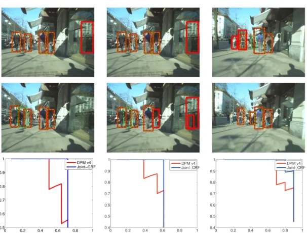
on test pairs of the Pedestrian dataset. Top two rows: Input image pairs (Green dash: our results, Red solid: DPM results); Bottom row: Precision-recall curves of our method and DPM for the three image pairs. . . 62 3.4 Predicting similarity: Sample similarity matrix obtained by

apply-ing our learned similarity function to one test pair of the Pedestrian dataset. Top: Input image pair; Middle: (Left) target (ground truth) similarity matrix, (Right) learned similarity matrix (brighter means more similar); Bottom: Normalized histograms of similarity scores for matched and non-matched candidate pairs. . . 63

3.5 Car co-detection Results: Examples of our co-detection results on test pairs of the Ford Car dataset. Top two rows: Input image pairs (Green dash: our results, Red solid: DPM results); Bottom row: Precision-recall curves of our method and DPM for the three image pairs. . . 64 3.6 Predicting similarity: Sample similarity matrix obtained by applying

our learned similarity function to one test pair of the Ford Car dataset. Left: Input image pair; Middle: (Top) target (ground truth) similarity matrix, (Bottom) learned similarity matrix (brighter means more sim-ilar); Right: Normalized histograms of similarity scores for matched and non-matched candidate pairs. . . 66 3.7 Category-specific object co-detection precision-recall curves: The

precision-recall curves over all pairs (Blue solid: our results, Red solid: DPM results). Left: Pedestrian dataset ; Right: Ford car dataset. . . 67 3.8 Sample Results:Examples of our co-detection results on two sets from

the Human Co-detection dataset. Top: Input image set overlaid with detection output (Green dash: our results, Red solid: DPM results); Bottom: Precision-recall curves of our method and DPM for the two sets. 67 3.9 Predicting similarity: Sample similarity matrix obtained by

apply-ing our learned similarity function to one test set in the Human Co-Detection dataset. Top: Input images (three examples); Middle: (Left) target (ground truth) similarity matrix, (Right) learned similarity ma-trix (brighter means more similar); Bottom: Normalized histograms of similarity scores for matched and non-matched candidate pairs. . . 68 4.1 Top: Conventional single-class object co-detection vs. Bottom: our

multi-class object co-detection approach. . . 72 4.2 Precision/Recall curves: Performance comparison on four

represen-tative categories using the VOC 2007 dataset. Blue curve represents the R-CNN (without bounding-box regression) [Girshick et al., 2014], whereas, Red curve shows our method results. . . 87 4.3 Sensitivity and Impact Analysis: Overall detailed performance

com-parison using different metrics (i.e., occlusion (acc), truncated (trn), size, aspect ratio (asp), view point and part visibility). The black dashed line indicates the overall average normalized precision APN. . . 88

4.5 CoDeT-G-DL detection trends. Following [Hoiem et al., 2012], we show the evaluation of the type of detection as the number of de-tections increases; The white areas correspond to the correct detec-tions; The blue areas represent the detections with localization error; The red areas correspond to confusion with a similar category; The green areas represent the confusion with a dissimilar category. Finally, the line plots show the recall as a function of the number of objects (dashed=weak localization, solid=strong localization). . . 91 4.6 CoDeT-G-DL vs. R-CNN-BB (Normalized) Scores. For each image,

we show the changes in scores before and after performing dense CRF inference with our learned structured kernels. Columns 1-3 depict examples where our CoDeT-G-DL algorithm improved the scores of R-CNN-BB. Example bounding boxes with increased confidence are shown in column 1-2, column 3 shows the cases where bounding box confidence is decreased. Column 4 shows examples where the R-CNN-BB scores are better than ours. Note that, as in the false positive anal-ysis of Fig. 4.8, these cases correspond to either parts of objects, or multiple objects of the same class. . . 92 4.7 CoDeT-G-DL top detections. We show the top-scoring detections in

decreasing order from left to right for 10 representative classes. If an image has multiple detections, only its top-scoring detection is shown. Note that our top-scoring detections correspond to accurate object lo-calizations. . . 93 4.8 CoDeT-G-DL top false positives. We show the top-scoring false

posi-tives in decreasing order from left to right for 8 representative classes. Note that our top scoring false positives belong to two main categories:

(i)Parts of objects are confused with complete objects due to high sim-ilarity with objects that are truly partially observed; andii)Bounding boxes containing multiple objects of the same category are confused with single objects due to high similarity with other boxes truly con-taining single objects. Note, however, that our top-scoring false posi-tives do not contain truly absurd detections. . . 93

5.1 Overview of our deep structured network for object proposal co-generation. Our model consists of one deep CNN module per object candidate, linked by a fully-connected CRF. . . 99

5.2 Detailed architecture of our deep structured network for object pro-posal co-generation. Each input image first goes through a series of convolutional layers, followed by Region-of-Interest (RoI) pooling cor-responding to the different candidates in the image. Each candidate then passes through several fully-connected layers to predict unary features, pairwise features and bounding box location offsets. The fea-tures are finally employed in a fully-connected CRF. During training, our model makes use of a multi-task loss. . . 100 5.3 Pascal VOC 2007 test: We compare our method with state-of-the-art

object proposal baselines according to the criteria of [Hosang et al., 2016]. Left: Recall v.s. IoU threshold. These recall curves were gener-ated using the highest-scoring 10, 100, 1000 and 10000 object proposals, respectively. Right: Recall v.s. Number of Proposals. The first plot shows the AR, and the remaining recall curves were generated using IoU thresholds of 0.5, 0.7 and 0.8, respectively. In all the plots, the dashed lines correspond to our co-generation results, in blue when using Selective Search candidates (Co-Obj (SS)) and in black when using Bing candidates (Co-Obj (B)). The baselines correspond to Bing (B), EdgeBoxes (EB70), Geodesic (G), MCG (M) and SelectiveSearch (SS). These results clearly evidence the benefits of our co-generation approach. . . 108 5.4 MS COCO validation: We compare our method with state-of-the-art

object proposal baselines according to the criteria of [Hosang et al., 2016]. Top: Recall v.s. IoU threshold. These recall curves were gener-ated using the highest-scoring 10, 100, 1000 and 10000 object proposals, respectively. Bottom: Recall v.s. Number of Proposals. The first plot shows the AR, and the remaining recall curves were generated using IoU thresholds of 0.5, 0.7 and 0.8, respectively. In all the plots, the dashed lines correspond to our co-generation results, in blue when us-ing EdgeBox candidates (Co-Obj (EB)) and in black when using Bing candidates (Co-Obj (B)). The baselines correspond to Bing (B), Edge-Boxes (EB70), Geodesic (G), MCG (M) and SelectiveSearch (SS). These results again evidence the benefits of our co-generation approach. . . . 110 5.5 Sensitivity and impact analysis: Overall detailed performance

com-parison using different metrics (i.e., occlusion, truncated, size, aspect ratio, view point and part visibility). The black dashed line indicates the overall average normalized precision APN. . . 112

5.6 Deep co-objectness and detection trends. Following [Hoiem et al., 2012], we show the evolution of the type of detection as the number of detections increases; The white areas correspond to the correct detec-tions; The blue areas represent the detections with localization error; The red areas correspond to confusion with a similar category; The green areas represent the confusion with a dissimilar category. Fi-nally, the curves show the recall as a function of the number of objects (dashed=weak localization, solid=strong localization). . . 113 6.1 Traditional instance segmentation vs our shape based

representa-tion. Left: Original image and ground-truth segmentation. Middle:

Given a bounding box, traditional methods directly predict a binary mask, whose extent is therefore limited to that of the box and thus suffers from box inaccuracies. Right: We represent the object segment with a multi-valued map encoding the truncated minimum distance to the object boundary. This can be converted into a mask that goes beyond the bounding box, which makes our approach robust to box errors. . . 118 6.2 Left: Truncated distance transform. Right: Our deconvolution-based

shape-decoding network. Each deconvolution has a specific kernel size (ks), padding (p) and stride (s). Here,Krepresents the number of binary maps. . . 120 6.3 Left: Detailed architecture of our boundary-aware instance

segmen-tation network. An input image first goes through a series of convo-lutional layers, followed by an RPN to generate bounding box pro-posals. After RoI warping, each proposal passes through our OMN to obtained a binary mask that can go beyond the box’s spatial ex-tent. Mask features are then extracted and used in conjunction with bounding-box features for classification purpose. During training, our model makes use of a multi-task loss encoding, bounding box, seg-mentation and classification errors. Right: 5-stage BAIS network. The first three stages correspond to the model on the left. The five-stage model then concatenates an additional OMN and classification module to these three stages. The second OMN takes as input the classifica-tion score and refined box from the previous stage, and outputs a new segmentation with a new score obtained via the second classification module. The weights of the OMN and classification modules in both stages are shared. . . 123

6.4 Qualitative results on Cityscapes From left to right, we show the in-put image, our instance level segmentations and the segmentations projected onto the image with class labels. Note that our segmenta-tions are accurate despite the presence of many instances. . . 128 6.5 Failure cases. The typical failures of our approach correspond to cases

where one instance is broken into multiple ones. . . 129 6.6 Recall v.s. IoU threshold on Pascal VOC 2012. The curves were

gener-ated using the highest-scoring 10, 100 and 1000 segmentation propos-als, respectively. In each plot, the solid line corresponds to our OMN results. Note that we outperforms the baselines when using the top 10 and 100 proposals. For 1000, our approach still yields state-of-the-art results at high IoU thresholds. . . 130

3.1 Pedestrian co-detection with stereo pairs: Comparison of our ap-proach with state-of-the-art co-detection methods on Pedestrian dataset using stereo pairs. . . 61 3.2 Pedestrian co-detection with random pairs: Comparison of our

ap-proach with state-of-the-art co-detection methods on Pedestrian dataset using random pairs. . . 61 3.3 Car co-detection with stereo pairs: Comparison of our approach with

state-of-the-art co-detection methods on the Ford Car dataset using stereo pairs. . . 64 3.4 Car co-detection with random pairs: Comparison of our approach

with state-of-the-art co-detection methods on the Ford Car dataset us-ing random pairs. . . 65 3.5 Human co-detection: Comparison of our approach with

state-of-the-art co-detection methods on the HCD dataset . . . 65 4.1 Detection average precision(%) on the PASCAL VOC 2007 test set

using AlexNet. Columns 1-2 shows the co-detection baselines i.e. MLRR [Guo et al., 2013] and MCOL [Desai et al., 2009]. Columns 3-4 provide the baseline state-of-the-art results for detection [Girshick et al., 2014]. R-CNN (without bounding-box regression); R-CNN BB (with bounding-box regression). Column 5 provides results of Chap-ter 3 co-detection method with deep network unary potentials. Columns 6-8 show co-detection performance. CoDet-G (R-CNN-BB with geo-metric context model learning); CoDet-G-LA (Kernel selection using max-margin learning); CoDet-G-DL (Kernel selection using direct loss minimization). . . 85 4.2 Detection average precision(%) on the PASCAL VOC 2007 test set

using VGG16. Column 1 shows the results of the Fast-RCNN baseline and Column 2 shows our method results using VGG16. . . 86

4.3 Multi-class average precision(%) on the PASCAL VOC 2007 test set.

CoDet-G-DL (Kernel selection using direct loss minimization). We con-structed the baseline curve for R-CNN-BB (with bounding-box regres-sion) [Girshick et al., 2014] by pooling the detections across all object classes and images when computing the PR curves. Our model clearly provides a noticeable boost in overall performance. . . 89 4.4 Detection average precision(%) on the PASCAL VOC 2012 test set.

Columns 1-2 provide the baseline state-of-the-art detection results![Girshick et al., 2014]. R-CNN (without bounding-box regression); R-CNN BB (with bounding-box regression). Columns 3-4 show our co-detection performance. CoDet-G (R-CNN-BB with geometric context model learn-ing); CoDet-G-DL (Kernel selection using direct loss minimization). . . 90 5.1 AR analysis on the PASCAL VOC 2007 test set: We compare our

method with state-of-the-art object proposal baselines according to the criteria of [Lin et al., 2014]. The results of our approach are provided in Rows 7-8 when using Bing and Selective Search to generate the initial candidates, respectively. The AR for small, medium and large objects were computed for 100 proposals. Note that our co-generation approach outperforms the state-of-the-art baseline in all metrics. The difference in speed between two versions of our approach is due to the fact that Bing yields a larger candidate pool than Selective Search. . . . 108 5.2 Using different initial proposal methods:Rows 1-2 show the baseline

object proposal methods. Rows 3-6 show our results using various candidate generation options at training and test time. . . 109 5.3 AR analysis on the MS COCO validation set:We compare our method

with state-of-the-art object proposal baselines according to the crite-ria of [Lin et al., 2014]. The results of our approach are provided in Rows 7-8 when using Bing and EdgeBox to generate the initial candi-dates, respectively. The AR for small, medium and large objects were computed for 100 proposals. Note that our co-generation approach outperforms the state-of-the-art baseline in all metrics. . . 110 5.4 Detection Average Precision(%) on the PASCAL VOC 2007 test set:

Columns 1-3 show the multi-class object detection state-of-the-art re-sults for Fast RCNN (SS) [Girshick, 2015], CoDet-G-DL (SS) of Chap-ter 4, RPN [Ren et al., 2015] and Fast RCNN (SS) respectively. The results of our approach are provided in Row 4. . . 111

6.1 Instance-level semantic segmentation on Pascal VOC 2012. Com-parison of our method with state-of-the-art baselines. The results of [Hariharan et al., 2014, 2015] are reproduced from [Dai et al., 2016b]. . . 126 6.2 Influence of the number of stages during training. Whether trained

using 3 stages or 5, our approach outperforms both MNC baselines. . . 127 6.3 Instance-level semantic segmentation on Cityscapes. We compare

our method with the state-of-the-art baselines on the Cityscapes test set. These results were obtained from the online evaluation server. . . . 127 6.4 Detailed comparison with DTW [Bai and Urtasun, 2017] at AP(50%).

Note that our approach outperforms this baseline on all the classes except truck and motorcycle for the Cityscapes test dataset. . . 128 6.5 Comparison with MNC-new on the Cityscapes validation data.Note

that our approach outperforms this baseline, thus showing the impor-tance of allowing the masks to go beyond the box proposals. . . 128 6.6 Evaluation of our OMN on the PASCAL VOC 2012 validation set.

We compare our method with state-of-the-art segmentation proposal baselines according to the criteria of [Hariharan et al., 2014; Lin et al., 2014]. Note that our approach outperforms the state-of-the-art meth-ods for the top 10 and 100 segmentation proposals, which correspond to the most common scenarios when later processing is involved, e.g., instance level segmentation. . . 130 6.7 Detailed Evaluation on the Pascal VOC 2012 validation set. We

re-port results with mask level IoU thresholds of 0.5 and 0.7. Note that our method outperforms MNC [Dai et al., 2016b] for most classes and achieves an improvement of 2.1% over MNC at a 0.7% IoU threshold . . 130 6.8 Object size analysis on the Pascal VOC 2012 validation set. We

com-pare our method with state-of-the-art segmentation proposal baselines according to the criteria of [Lin et al., 2014]. The AR for small, medium and large objects were computed for 100 proposals. Note that our ob-ject mask network outperforms the state-of-the-art baselines for large objects by a significant margin. . . 131 6.9 Qualitative results on Pascal VOC 2012. From left to right, we show:

the original image, the segmentations of MNC, these results projected on the image, our segmentations, our results projected on the image. Note the better quality of our results. . . 132

2.1 Mean field in fully connected CRFs [Krähenbühl and Koltun, 2011] . . . 24 4.1 Structural Kernel Learning Algorithm . . . 82 5.1 Mean-field Gradient for Classification Loss . . . 106

Introduction

Image and scene understanding is one of the most important unsolved problems in computer vision, and the complexity of real environments makes it challenging to interpret natural images and videos. Diagnosing brain cancer by detecting and analysing medical images, safe navigation for an autonomous vehicle and landing the Curiosity rover on Mars by detecting and avoiding the obstacles using vision sensors are only a few examples of the numerous applications that all require arti-ficial systems that mimic the human vision system to accurately extract high-level information from images. Decoding natural scenes into objects and their interactions relies on addressing the intermediate vision challenges of object detection, recogni-tion and segmentarecogni-tion. In recent years, the availability of large scale natural image datasets, e.g., Image-Net [Krizhevsky et al., 2012], Pascal VOC [Everingham et al., 2010; Everingham et al.], Microsoft COCO [Lin et al., 2014] and Cityscapes [Cordts et al., 2016], and the statistical models inspired by efficient machine learning tech-niques have shown impressive progress by achieving compelling and accurate results in solving the most complex visual computing challenges, but they are still far from matching the human brain’s remarkable performance.

Over the years, the techniques proposed to achieve the intermediate goals of image and scene understanding were mostly focused on single image techniques and much work has been done to address the problem of object detection by either class-specific methods [Felzenszwalb et al., 2010] or using object proposal genera-tion methods [Girshick, 2015; Ren et al., 2015; He et al., 2015]. Generating class-independent object proposals, based on objectness measures, facilitates detection by proposing a smaller number of interesting candidate regions. Whether class-specific or class-independent, most existing methods make decisions on individual objects to perform detection. Such a myopic view, however, is too restrictive as it ignores all structural and contextual information, and the appearance of natural objects is often ambiguous due to the lack of context, poor resolution, occlusions, or challenging lighting conditions.

Context-aware deep structured modelsare important because they tend to learn semantic contents accurately and efficiently by analysing an entire image or multi-ple images jointly. Recently, small scale context-aware models in image parsing have gained wide popularity. Context-aware foreground-background image segmenta-tion [Nowozin and Lampert, 2011; Blaschko and Lampert, 2012] is the task of pre-dicting pixel-level correspondences given some image or video data. In structured prediction, probabilistic graphical models provide a powerful framework to learn the dependence structure between variables, which can be represented as a graph. Typically, vertices of graph represents the nodes (pixels or superpixels) and edges encode the neighborhood relations. The task is to produce a consistent labeling of all the vertices. Modeling and learning these structured and contextual models us-ing large-scale data is very challengus-ing. A number of methods have been proposed [Bengio, 2012] to obtain computationally feasible solutions, but are complicated by several factors. In particular, given a large graph with millions of nodes, the input and output spaces tend to have exponential number of possibilities and performing inference using millions of interrelated variables is difficult and time consuming.

High performance computing using a graphics processing unit (GPU) is vital and is at the heart of the emerging visual computational techniques. GPU-accelerated deep learning utilizes parallel computation on GPU to significantly reduce the time it takes to learn these models. The advent of the NVIDIA CUDA deep neural network library (cuDNN) [NVIDIA, 2015] has led to a surge of interest for research in increas-ingly effective techniques for object detection, localization and recognition. Learning an end-to-end deep structured model requires an enormous amount of computation and time, and proper utilization of GPU computation power makes it possible to learn these useful models efficiently.

In this thesis, we focus on structured prediction and propose and validate efficient deep structured models for context-aware object detection, localization and segmen-tation. Context-aware image analysis has a major impact on applications that rely on the analysis of large scale multi-image data. Visual question answering, image based content retrieval and video based self-learning cannot be achieved without knowing the context. In addition, context aware instance detection/segmentation is a funda-mental research topic since it constitutes a critical step for many complex processes, such as segmenting MRI images for cancer treatment, multiple camera fusion for tracking, autonomous navigation and free-viewpoint film production.

Before presenting our contributions, we briefly review a few examples of com-puter vision challenges that we intend to study, in this thesis, by using context-aware deep structured models.

1

.

1

Some Computer Vision Challenges

Here we briefly discuss some core computer vision challenges that are building blocks for image understanding and scene analysis. We will formally define the methods developed over the years in Chapter 2. However, for better understanding, we first briefly outline some of the applications and how they are related to each other in this section.

1.1.1 Object Detection

Object modeling and recognition has been one of the fundamental problems in com-puter vision since its early days [Dickinson et al., 2009]. Numerous methods have been proposed to tackle this task which can be categorized into two broad categories: one that rely on hand-crafted representation,e.g., [Viola and Jones, 2004], and others that automatically learn representations from data,e.g., [Girshick, 2015]. In particu-lar, object detection has evolved into a core challenge in vision research [Everingham et al., 2010], and much progress has been made recently due to advances in de-formable part-based object models, e.g., DPM [Felzenszwalb et al., 2010], as well as in deep network based models [Girshick et al., 2014].

Figure 1.1: An illustration of a pedestrian detection system. It takes a single image as input and provides a list of all pedestrians.

Given an image and an object category list, the goal of object detection is to find all the relevant individual objects in the image. An example of this is illustrated in Figure 1.1. These predicted objects usually have a unique location in the input image and are marked with a bounding-box in the output image. Object detection in the wild is a challenging task because of the complexity of unconstrained envi-ronments, large viewpoint variations, object occlusions, motion, deformations and lighting variations.

1.1.2 Object Co-detection

Object co-detection methods [Bao et al., 2012; Guo et al., 2013; Shi et al., 2013] were recently introduced to exploit the collective power of a set of images. In contrast to

object detection, object co-detection techniques jointly process multiple images at test time and find all objects collectively. This is illustrated in Figure 1.2. The benefits of jointly processing multiple images is that it can help model complex environments with large viewpoint variations, and can overcome object detection limitations, such as occlusions, deformations and lighting variations.

Figure 1.2: An illustration of a pedestrian co-detection system. It takes multiple images as input at test time and provides a collective list of all pedestrians.

1.1.3 Objectness

Traditionally, object (co-)detection methods take a scanning window approach and exhaustively search for object candidates at every location and scale in an image [Vi-ola and Jones, 2004; Dalal and Triggs, 2005; Felzenszwalb et al., 2010]. More recently, objectness criteria have been used to propose potential candidates, which drastically reduces the search space [Endres and Hoiem, 2010; Alexe et al., 2010; Uijlings et al., 2013]. Objectness, however, is very challenging to adequately represent, since it has to account for the huge intra-class variations of the generalobjectcategory, while still being able to differentiate it from thebackgroundclass. As a matter of fact, these chal-lenges remain unsolved even when detecting specific objects. Objectness methods are generally categorized based on the type of output they produce.

1.1.3.1 Box Proposals

Box proposal methods provide just a bounding-box around a potential object in-stance. This is often desired when learning a class-generic object detector. An illus-tration using selective search [Uijlings et al., 2013] is shown in Figure 1.3 (Left).

1.1.3.2 Segment Proposals

Segmentation proposal methods provide not only the bounding-box around a poten-tial object instance but also a pixel-level labeling that separates the instance from its

Figure 1.3: An illustration of class-agnostic box and segmentation proposal meth-ods. Left: An example with the selective search technique [Uijlings et al., 2013]. It takes a single image as input and provides a list of all potential objects. Right: An example with the sharp-mask technique [Pinheiro et al., 2016]. It takes a single image as input and provides a list of all potential segments.

background inside that bounding-box. This is often desired when designing an in-stance segmentation method. An illustration using the sharp-mask method [Pinheiro et al., 2016] is shown in Figure 1.3 (Right).

1.1.4 Semantic Segmentation

Semantic segmentation is the task of partitioning an input image into segments re-lated to multiple categories. In contrast to object (co-)detection techniques, it pro-vides a detailed pixel-level view of the scene and is useful for many scene under-standing tasks. A limitation of semantic segmentation is that it ignores the bound-aries between the individual objects. A sample semantic segmentation is shown in Figure 1.4. Note that each object category is represented by a different color.

Figure 1.4: An illustration of a semantic segmentation. Left: An image from Pascal VOC 2012 [Everingham et al.], andRight: Ground-truth pixel-wise labeling.

1.1.5 Semantic Instance Segmentation

Semantic instance segmentation is the task of segmenting/detecting individual ob-jects along with their exact pixel-wise outline in the scene. In contrast to semantic segmentation, it distinguishes the individual instances of the same category. This is a very challenging task since the number of objects are not known and varies from im-age to imim-age. Furthermore, instance segmentation is often termed as simultaneous detection and segmentation and provides useful insights about the objects in con-text. A sample instance segmentation is shown in Figure 1.5. Note that each object instance is represented by a different color.

Figure 1.5: An illustration of semantic instance segmentation. Left: An image from Pascal VOC 2012 [Everingham et al.]. Right: Ground-truth pixel-wise instance semantic labeling.

1

.

2

Contributions

In this thesis, we introduce new algorithms to learn context-aware models for im-proving the accuracy of object detection, localization and instance segmentation. The goal of the proposed methods is to introduce algorithms for efficiently processing large scale image datasets with an emphasis on the quality and robustness of the results when compared with the state-of-the-art methods. The contributions are four-fold: first, we present a novel class-specific similarity learning algorithm that can be used to jointly process large scale datasets for efficient object co-detection; second, we extend our method to multi-class similarity learning and further leverage deep features and geometric scene layout, thus providing a novel algorithm for large scale object detection in context; third, we introduce a class-agnostic object similar-ity formulation for overcoming the poor localization performance of object detectors and provide a solution that learns context jointly within a deep structured network;

fourth, we develop a boundary-aware instance segmentation approach which not only can predict segmentation mask inside a bounding-box but also can go beyond it, which is a major limitation of most existing state-of-the-art approaches. Specifi-cally, we discuss how our algorithms address the limitations of the existing ones.

• Learning Category-Specific Object Similarity: We introduce a principled for-mulation of object co-detection as an efficient inference in a fully-connected CRF whose nodes represent object candidates and edges encode the object sim-ilarity. We demonstrate that modeling the similarity between pairs of candi-dates as a weighted mixture of Gaussian kernels allows us to efficiently perform inference in large graphs optimally. As a result, our approach can effectively leverage the information in multiple images to improve detection accuracy, thus outperforming existing co-detection techniques on benchmark datasets.

• Multiclass Structural Kernel Boosting: We extend our co-detection algorithm to handle multiple object classes simultaneously in large scale image datasets. The unified framework to jointly learn a CRF and interclass similarity based on deep features allows us to yield better performance. Furthermore, our struc-tural boosting strategy lets us benefit from rich, high-dimensional features to learn the contextual relationships within our CRF framework. Empirical com-parisons show that our method outperforms state-of-the-art object detection methods on Pascal VOC 2007 and 2012.

• Class-agnostic Similarity Learning with a Deep Structured Network: We present an end-to-end learning algorithm to jointly generate object proposals from multiple images, thus leveraging the collective power of multiple object candidates. In contrast to most existing methods, our method is based on a deep structured network that jointly predicts the objectness scores and the bounding box locations of multiple object candidates by extracting features that model the individual object candidates and the similarity between them. Em-pirical comparisons show the benefits of our approach over the state-of-the-art methods that generate object proposals individually.

• Beyond Boxes: Boundary-Aware Instance Segmentation: We develop a dis-tance transform-based mask representation that allows us to predict insdis-tance segmentations beyond the limits of initial bounding boxes. Subsequently, we present an efficient approach to infer and decode this representation with a fully-differential Object Mask Network (OMN) which inherently relies on a residual-deconvolutional architecture. This modular approach allows us to em-ploy this OMN module into an instance segmentation framework. To the best

of our knowledge, this constitutes the first method that can segment instances beyond the bounding-box limit. Furthermore, our quantitative and qualitative experiments demonstrate the superiority of proposed approach over the state-of-the-art instance-level semantic segmentation methods.

1

.

3

Thesis Structure

In this chapter, we provided a brief overview of challenging applications that benefits from our research. Following this introduction chapter, the remaining chapters of the thesis are summarized below.

Chapter2. This chapter starts with an overview of supervised learning and intro-duces the basic notations. Furthermore, we provide an overview of fundamental structured learning models and review relevant state-of-the-art techniques. We also present techniques to compute hand-engineered representations as well as automat-ically learned deep representations. In particular, we discuss conditional random fields to incorporate structure and contextual information, formalize feature learn-ing and later discuss the popular deep convolutional neural network architectures. In the end, an overview of large scale challenging image datasets and respective evaluation metrics is also provided. Note that the material included in this chapter is intended for readers who are not familiar with related concepts and methods used in rest of the thesis. However, readers with relevant background may skip this chapter.

Chapter3. This chapter is based on our work [Hayder et al., 2014] to learn category-specific object similarity. Here, we formulate object co-detection as inference in a fully-connected conditional random field (CRF) whose edges model the similarity between object candidates. Furthermore, we demonstrate the scalability of our algo-rithm compared to existing co-detection techniques that rely on exhaustive or greedy search.

Chapter4. This chapter is based on our work [Hayder et al., 2015] that extends our model in Chapter 3 to learn multi-category object similarity. Here, our structural boosting strategy lets us benefit from rich, high-dimensional features to learn the object relationships within our CRF framework, thus lead to superior object (co-)detection results. Note that, in last chapter, although we start with simple-yet-effective hand-crafted object features to learn the similarity, here, we model object instances with features learned using deep neural network to improve the quality of our similarity learning algorithms.

Chapter 5. This chapter is based on our work [Hayder et al., 2016] that learns a class-agnostic geometric model and instance similarity jointly to improve the accu-racy of object detection and localization. Here, we develop an end-to-end learning algorithm that, by unrolling the CRF inference procedure, lets us backpropagate the loss gradient throughout the entire structured network, thus learning better contex-tual features for detection.

Chapter6. This chapter is based on our work [Hayder et al., 2017] that introduces a novel representation based on the distance transform of the object masks. Here, we design an object mask network with a new residual-deconvolution architecture that infers such a representation and decodes it into the final binary object mask. This allows us to predict masks that go beyond the scope of the bounding boxes and are thus robust to inaccurate object candidates.

Chapter7. In this chapter, we draw conclusions based on the observations made in previous chapters and suggest several future research directions.

1

.

4

Publications

The contributions described in this thesis have previously appeared in the following publications.

• Z. Hayder, X. He and M. Salzmann, "Boundary-aware Instance Segmentation",

The IEEE Conference on Computer Vision and Pattern Recognition (CVPR), July

2017.

• Z. Hayder, X. He and M. Salzmann, "Learning to co-generate object proposals with a deep structured network", The IEEE Conference on Computer Vision and Pattern Recognition (CVPR), June 2016.

• Z. Hayder, X. He and M. Salzmann, "Structural kernel learning for large scale multiclass object co-detection", The IEEE International Conference on Computer Vision (ICCV), December 2015.

• Z. Hayder, M. Salzmann and X. He, "Object co-detection via efficient inference in a fully-connected crf", The European Conference on Computer Vision (ECCV), September 2014.

Background and Preliminaries

The role of this chapter is to provide fundamental concepts and an overview of structured models. This chapter starts with an overview of the basic notation and terminology used for learning supervised models. We build upon this and provide an overview of fundamental structured learning models and review relevant state-of-the-art techniques. We also present techniques to compute hand-engineered rep-resentations as well as automatically learned deep reprep-resentations. In particular, we discuss conditional random fields to incorporate structure and contextual informa-tion, deep feature learning and later discuss the popular deep convolutional neural network architectures. In the end, an overview of large scale challenging image datasets and respective evaluation metrics are also provided.

2

.

1

Supervised Learning

The idea of inferring from examples, or labeled data, is typically formulated as su-pervised learning. In susu-pervised learning, the main focus is on accurate prediction and to perform well on previously unseen data. Generally, the datasetD consists of

ndata and label pairs{(Xn,yn)}={(x1,y1),(x2,y2), ...,(xn,yn)}, where eachxi ∈ Rd

is a real-valued vector of d dimensions representing features of a single data point, andy_i is the given label for that datum.

Given a training setDwith input attributes setXn={x1,x2, ...,xn}and a nominal

target attributeyn ={y1,y2,· · · ,yn}from an unknown fixed distributionP over the

labeled instance space, the goal is to induce an optimal classifier with minimum generalization error.

The dataset D is divided into multiple sets to quantify if the model generalizes well to previously unseen examples. In this sense, one distinguishes between the data that is used to train a model, validate its performance, and to test the trained & validated model. These sets are commonly named as the training {Xtrain,ytrain},

validation{Xval,yval}and test{Xtest,ytest}set.

Given a training dataset, the goal of supervised learning is to learn the complex relationship or a function between inputXand the outputy, i.e., fθ :X→y, such that

ypred = f(X|θ) is a good predictor for the corresponding y. For historical reasons, this function f is called the hypothesis and the model parameters are denoted by θ. In supervised learning, our interest is learning a good hypothesis f such that it not only accurately classifies the xi in the training data but also classifies new samples

x from the distribution (x,y)∼ P reasonably well. In a typical supervised learning scenario, learning a good hypothesis f from data is an iterative process and it usually performs the following basic steps

• GivenXtrain, learn a model ˆfθ that best predicts the label vectorytrain.

• Validate the model usingXval and find the best parametersθ.

• Test the model usingXtest and compute the model accuracy.

For example, in a license plate recognition system (LPR), xi might be a vector

representing a scanned image of a car’s number plate with English letters and many numerical digits. The corresponding label yi might be a the supervised learning

output of the image as a vector of alphanumeric characters. The goal is to learn the inherent relationship in the training set and to make intelligent guesses about the labels for the image by making intelligent guesses from the training set.

Loss function: In learning, a loss function L(X,y,f(X)) is very important and is explicitly specified to gauge the accuracy of a classifier f and it is a measure of how well f classifies X when the true label is y. In an ideal scenario when the learned function accurately predicts all the data-points, e.g., f(X) = y, the loss is zero, i.e.,

L(X,y,f(X)) =0.

The most common loss is called the 0/1 loss defined as

L0/1(X,y, f(x)) =I(y6= f(X)), (2.1) where I(·)denotes the indicator function, i.e.,I(t) =1 ift is true and 0 otherwise. The empirical riskR_(L,P)(f)of the classifier f can be calculated as

R_(L,P)(f) = 1 n n

∑

The generalization error is defined as the misclassification rate over the distribu-tion P. The classification accuracy of a classifier is one minus the expected loss or generalization error. The training error is defined as the percentage of examples in the training set correctly classified by the classifier. This is often calculated on the

entire training set, although, in recently famous deep learning frameworks, this is usually calculated on mini- batches.

Regularization: Choosing a classifier f with the minimum empirical risk could be misleading due to two main reasons. First of all, it assigns equal weight to all data samples irrespective of their label frequency. Secondly, a naive classifier might over-fit to the training data, i.e., it might have zero classification loss on the training dataset D, but very high loss on test set, which occurs due to poor generalization performance of the classifier on unseen data. Therefore, aregularizationterm is often introduced to avoid the problem of over-fitting and as a trade off between the risk of the classifier and the complexity of the hypothesis. In particular, given a set of hy-potheses F, the best hypothesis is selected by minimizing the regularized empirical risk as

f∗ =argmin

f∈F

R_(L,P)(f) +λΩ(f), (2.3) where λ is a trade-off factor called the regularization parameter. The regularizer is represented by Ω(f) and is generally a non-negative function which penalizes the inherent complexity of the classifier f. If the hypothesis classF is very large and complex, the search for the optimal f∗in Equation 2.3 can become a very challenging task. In particular, finding the optimal hypothesis becomes intractable due to the exponential size of the label space. For these intractable classes, it becomes very important to choose a fast searching procedure or an efficient inference technique, for the algorithm to remain tractable.

Classification v.s. Regression: The learning problem is often called a regression

problem when the target variable yis continuous, i.e.,y∈ R. However, it is termed

a classification problem when y is one of a discrete number of possible values

of-ten called class labels, generally represented by c, i.e., y ∈ {0, 1, ...,c}. Examples of techniques that have been proposed in the past for supervised learning include

linear/non-linear regression,decision trees,support vector machines,naive bayesandneural networks. Binary and multi-class classification have been the focus of general super-vised learning methods.

Curse of dimensionality: In most computer vision problems, images are the most predominant form of data used for supervised learning algorithms. These images are often preprocessed to compute properties, often called features, representing the images in a compact form. The size of the parameter search space increases

expo-nentially with the high dimensionality of these input features, and thus increases the chance that the classification algorithm will find spurious classifiers that are gener-ally invalid. Indeed, the required number of labeled samples for supervised clas-sification increases as a function of dimensionality [Jimenez and Landgrebe, 1998]. This phenomenon is usually called the curse of dimensionality [Bellman, 1957]. An interesting example of this phenomenon are decision tree classifiers. Although the efficiency of binary decision trees is very high in low dimensions, they fail to main-tain this performance when the number of dimensions increases beyond a cermain-tain limit. Interestingly, classifiers with fewer features are much more efficient to learn and their is less chance of over-fitting to the data. In this line of research, a number of dimensionality reduction techniques have been proposed, e.g., Linear discriminant analysis [Riffenburgh and Clunies-Ross, 1960], Principal component analysis [Dun-teman, 1989], Independent component analysis [Hyvärinen et al., 2004], and Robust PCA [Candès et al., 2011]. Indeed, learning compact representations in itself is a very challenging problem.

Computational complexity: An important criterion for comparing the performance of different supervised learning techniques is to take into account their computa-tional complexities. Formally, this is defined as the amount of CPU cycles or GPU time used at time of training and testing. Typically, the inference complexity at test time is important since it measures exactly how well a technique will scale with the amount of test data especially when massive datasets are used. Testing complexity can be critical especially for certain real time applications. Since most of the algo-rithms have worse than linear computational complexity, dealing with large scale datasets requires efficient inference algorithms.

In this section, we have defined a general supervised learning problem and the important terms related to learning a better classifier. However, with increasing complexity of data with multiple, complex and correlated labels structured predic-tion and Bayesian analysis methods often provide better generalizapredic-tion guarantees. In the next sections, we provide an overview of structured prediction learning and a general formulation to model these problems using probabilistic graphical models.

2

.

2

Structured Prediction

Real world data exhibits complex relations and strong correlations between different parts of an input. Structured prediction deals with the problem of classifying struc-tured outputs and/or multiple, interdependent outputs. Essentially, it deals with data with inherent structure and often described as a generalization of the

proba-bilistic inference task. This is in contrast with supervised learning, as discussed in the previous chapter, where inference is performed to learn the functional dependen-cies between inputs and outputs from training data.

Formally, for an input domain X and a structured output domain Y, structured prediction is defined as predicting f(X) by maximizing an underlying function g,

i.e.,

y∗= f(X) =argmax

y∈Y

g(X,Y). (2.4) Finding the optimal y∗ in the above equation is generally termed as inference or prediction. However, the function g(X,Y) is often formulated using a linear parametrization of model parameters θ and with a learnable feature function Φ, which yields

y∗ = f(X) =argmax

y∈Y

θTΦ(X,Y). (2.5) Interestingly, the output space has inherent structure and label dependencies that encode interesting concepts rather than a single discrete value. This is in contrast with the previous section, in which data consists of several parts, here, not only the parts themselves contain information, but also the configuration in which the parts belong together,e.g., on a spatial grid. An example of this problem is pixel-wiseimage

segmentation, where an individual pixel often doesn’t contain enough information on

its own but can benefit from dependencies with its neighbouring pixels.

It is important to note that the structured prediction problems are often formu-lated using graphical models. Also, the model parameters θ and feature function

Φ are generally learned using efficient inference techniques in probabilistic graph-ical models. Here, we first briefly describe essential concepts related to statistgraph-ical inference. It rests on the assumption that prior knowledge can be incorporated in the model parameters. The key ingredients to statistical inference are theprior distribution

and thelikelihood function.

Prior distribution: A prior distribution quantifies the uncertainty about the param-eters before any data is observed. The model paramparam-eters θ is a random vector and is assumed to have a probability distribution. The prior distribution is generally represented as p(θ |α)whereαis a vector of hyper-parameters.

Likelihood function: A likelihood function p(X | θ) (often simply the likelihood) is a function of the parameters of a statistical model and of the data. Likelihood functions play a key role in statistical inference.

Conditional probability: The conditional probability is formally defined as

Definition 2.2.1. LetX andY be any two events in a sample spaceSwithP(Y)>0. The conditional probability ofY givenX is written p(Y | X)and is defined by

p(Y | X) = p(Y ∩ X)

p(X) . (2.6)

Bayes’ theorem: Bayes’ theorem, also known as Bayes’ rule, relates conditional probabilities of multiple events and provides a rule to update or revise the strengths of evidence-based beliefs when a new evidence becomes available. It gives a formula to find the conditional probability of an event p(Y | X), say, when the "reverse" conditional probability p(X | Y)is the probability that is known. Formally,

Definition 2.2.2. Let the eventsy1,y2,· · · ,ykbe disjoint and exhaustive events in the

sample space S , such that p(yi) > 0 , and let X be an event such that p(X) > 0.

Then according to Equation 2.6,

p(yi | X) =

p(X |yi)p(yi)

p(X) . (2.7)

In the remainder of this section, we present a principled way to encode the re-lationships between the structured outputs using graphical models such as Markov random fieldsandConditional random fields.

2.2.1 Probabilistic Graphical Models

Graphs are an intuitive way of representing the relationships among a large set of random variables. A graphical model is a representation of the probability distribu-tion in a way that the distribudistribu-tion can encode the condidistribu-tional independence structure of a large number of variables with graphs [Koller and Friedman, 2009]. It is an intu-itive and computationally useful way to reason about probability by abstracting out the parametric details from the conditional dependence relationships between the variables. In a graphical model, given some observations the goal is to estimate the best solution among all feasible solutions by encoding the joint or conditional prob-ability distribution. Furthermore, prior probprob-ability distributions let us incorporate knowledge and some additional assumptions [Nowozin and Lampert, 2011].

There are two kinds of graphical models; those based on directed graphs and those based on undirected graphs. The models represented by directed graphs are typically termed asBayesian networksand the undirected graph models are known as

Markov random fields. The following sections provides a brief overview of these two

2.2.1.1 Bayesian Networks

A Bayesian network is a graphical model that represents random variables along with their conditional dependencies with a directed acyclic graph (DAG) [Koller and Friedman, 2009]. The distribution is represented by variables that are the nodes in the graph and the directed edges between the nodes describe the conditional depen-dencies. The model represents a factorization of the joint probability of all random variables. More precisely, given a set of variables Y= {y1,· · · ,yn}, the joint

proba-bility distribution forYfactorizes into the following form

p(y) = n

∏

∑

We useyi to denote both the variable and its corresponding node, and ˆyi to denote

the parents of node yi. Together, these components define the joint probability

dis-tribution for Y. Equation 2.8 shows the conditional probability factorization of the joint probability distribution, which can be further factorized into prior probabilities and conditional probabilities.

Figure 2.1 shows an example of a simple Bayesian network with 5 random vari-ables. The joint probability of the variablesX= {A,B,C,D,E}is given by

p(A,B,C,D,E) = p(A)p(B)p(C|A,B)p(D|B,C)p(E|C,D). (2.10) It is interesting to note that the Bayesian network structure allows us to ignore

Figure 2.1: Example of a Bayesian network [Friedman et al., 1997] represented by a directed acyclic graph. The nodes correspond to random variables and the edges represent statistical dependencies between the variables.

certain dependencies if we already know the value of certain nodes in the network. The structure of the factorization that the network implies will restrict the different possibilities of what distributions we can have that fit the model [Koller and Fried-man, 2009]. However, the directed edges in a Bayesian network are used to capture only the causal relationships between random variables. It cannot be used to model the correlation relationships between random variables. Therefore undirected graph-ical models (Markov Random Fi