Discovering gated recurrent neural network architectures

(1)

DISCLAIMER:

This document does not meet

the

current format guidelines

of

the

Graduate School at

The University of Texas at Austin.

It has been published for

(2)

The Dissertation Committee for Aditya Rawal certifies that this is the approved version of the following dissertation:

Discovering Gated Recurrent Neural Network Architectures

Committee:

Risto Miikkulainen, Supervisor

Scott Niekum

Aloysius Mok

(3)

Discovering Gated Recurrent Neural Network Architectures

by

Aditya Rawal,

Dissertation

Presented to the Faculty of the Graduate School of the University of Texas at Austin

in Partial Fulfillment of the Requirements

for the Degree of

Doctor of Philosophy

The University of Texas at Austin May 2018

(4)

(5)

Acknowledgments

This work wouldn’t have been possible without unwavering support of my wife Neha, my father Jatin, my brother Kandarp and my 3-year old daugh-ter Samyra.

Risto , my advisor, has provided me freedom to fail which I found very encouraging. He has provided supported even during the most difficult periods of this endeavor. His guidance helped me pivot my efforts at the right time. He has been a role model and I wish to carry forward my learnings from him as I embark on a new chapter of my life.

(6)

Discovering Gated Recurrent Neural Network Architectures

by

Aditya Rawal, Ph.D.

The University of Texas at Austin, 2018 Supervisor: Risto Miikkulainen

Reinforcement Learning agent networks with memory are a key component in solving POMDP tasks. Gated recurrent networks such as those composed of Long Short-Term Memory (LSTM) nodes have recently been used to improve state of the art in many supervised sequential processing tasks such as speech recog-nition and machine translation. However, scaling them to deep memory tasks in reinforcement learning domain is challenging because of sparse and deceptive reward function. To address this challenge first, a new secondary optimization objective is introduced that maximizes the information (Info-max) stored in the LSTM network. Results indicate that when combined with neuroevolution, Info-max can discover powerful LSTM-based memory solutions that outperform tradi-tional RNNs. Next, for the supervised learning tasks, neuroevolution techniques are employed to design new LSTM architectures. Such architectural variations in-clude discovering new pathways between the recurrent layers as well as designing new gated recurrent nodes. This dissertation proposes evolution of a tree-based encoding of the gated memory nodes, and shows that it makes it possible to ex-plore new variations more effectively than other methods. The method discovers nodes with multiple recurrent paths and multiple memory cells, which lead to sig-nificant improvement in the standard language modeling benchmark task. The dissertation also shows how the search process can be speeded up by training an LSTM network to estimate performance of candidate structures, and by encourag-ing exploration of novel solutions. Thus, evolutionary design of complex neural network structures promises to improve performance of deep learning architec-tures beyond human ability to do so.

(7)

Chapter 1

Introduction

Imagine artificial agents that can learn from past events and adapt like hu-mans. These agents can then be deployed in challenging unseen environments. Robots with a sophisticated understanding of natural language and conversation skills can carry out many of our daily chores. Better weather forecasting systems that predict natural disasters can save many lives. One common technology that is critical in order to achieve these breakthroughs is AI based memory. With the help of recent many advancements in deep learning, recurrent neural networks have come to the forefront for building such AI based memory. The goal of this dissertation is to devise new techniques to further improve this field and discover better memory networks.

1.1

Motivation

Natural organisms can memorize and process sequential information over long time lags. Chimpanzees and orangutans can recall events that occurred more than a year ago (Martin-Ordas et al. ((2013)). Long term social memory can pro-vide significant survival benefits. For example, bottlenose dolphins can recognize each other’s whistle sounds even after decades (Bruck ((2013)). Such a capability allows the dolphin to identify adversaries as well as potential teammates for hunt-ing. First step towards adaptive behavior is to memorize past events and utilize them for future decision making (Stanley et al. (2003)). For example, a group of hyenas, during lion-hyena interactions, modulate their behavior over a period of time through memory-based emotions - transitioning from being fearful initially to becoming risk-taking later (Watts and Holekamp ((2008)). Memory is therefore a key cognitive component and incorporating this capability in artificial agents can make them more realistic (Schrum et al. (2011)).

In the reinforcement learning (RL) domain, the tasks requiring memory can be formally be described as POMDP problems. Traditionally, recurrent neural net-works (RNNs) have been the preferred choice for this purpose. However, RNNs leak information and are unable to discover long-term dependencies (Hochreiter

(11)

et al. (2001)). Long Short Term Memory (LSTM) (Hochreiter and Schmidhuber (1997a)) successfully overcomes these limitations of RNNs. It consists of memory cells with linear activations. The inflow and outflow of information to and from these cells is controlled by associated input/output gated units.

Such LSTM based memory networks are also used to build chat-bots, speech recognition and forecasting systems. The time-series prediction problem in such settings fall into the category of supervised learning problems. With the recent ad-vances in deep learning, the performance of such LSTM networks has improved drastically ( Bahdanau et al. (2015a), Graves and Jaitly ((2014)) but their capabili-ties cannot match human levels.

New methods are presented in this dissertation that can evolve deep se-quence processing recurrent networks to solve RL and supervised memory tasks with long time-dependencies.

While LSTM networks have been used to achieve strong results in the super-vised sequence learning problems such as in speech recognition (Graves and Jaitly ((2014)) and machine translation Bahdanau et al. (2015a), their success in POMDP tasks has been limited (Bayer et al. (2009a), Bakker et al. (2003)). A possible reason is that it is difficult to train LSTM units (including its associated control logic) with weak reward/fitness signal. Also, the number of LSTM units in a network is a pa-rameter that is often manually selected. This approach turns out to be inefficient especially in new problems where the memory depth requirements are not clear.

1.2

Challenges

In RL tasks, recurrent networks are often used as policy controllers to de-termine agent actions given some input observations or as function approxima-tors to predict the value function ( Hausknecht and Stone (2017)). However, one key challenge is to find the optimal size of such networks (for e.g. the number of nodes in the layer). This is not a straightforward task and requires separate hyper-parameter tuning. Size of the network matters for two reason: computational cost and performance. Larger networks have bigger memory footprint and they take more processor power. Networks used for RL are much smaller and run on CPU than the ones used for supervised learning (that use GPU). It becomes more critical

(12)

therefore for RL memory networks to have close to optimal network size. Selecting a model with a large number of LSTM nodes (much more than that required by the task) can lead to overfitting of the model while selecting a very small model can lead to underfitting.

A second challenge in solving RL memory problems could be that of sparse and deceptive rewards. Deceptive fitness landscapes often lead the agent to local optima. The lack of sufficient rewards can prevent the agent to escape local optima. The LSTM networks used for supervised learing are significantly larger than RL and the parameter size is often in the order of tens of millions. For su-pervised learning problem, backpropagation through time (BPTT) is a powerful technique to train LSTM network weights. With the availability of large scale la-beled data and GPU compute, it is now possible to train LSTMs with mini-batch stochastic gradient descent (SGD). Such networks often consist of couple of LSTM layers stacked together along with some glue logic (for e.g. embedding layer, soft-max layer) to construct a full model. These models can then be deployed for lan-guage modeling, machine translation, speech recognition etc.

Previously, experimental results in supervised non-recurrent tasks like im-age classification have demonstrated that deeper and larger feedforward networks often outperform smaller and shallower networks ( Saxe et al. (2013)). However, the same idea does not directly scale to deep recurrent networks. While, recurrent networks are naturally deep in time (depth equal to the number of unroll steps in BPTT), stacking more LSTM layers vertically yields diminishing returns ( Chung et al. (2015)). Some of the recent human designed variants of stacked LSTMs like recurrent highway networks ( Zilly et al. (2016)), grid LSTMs ( Kalchbrenner et al. (2015)) and gated-feedback networks ( Chung et al. (2015)) suggest that the search space of architecture is large. ( Chung et al. (2015)) and ( Kalchbrenner et al. (2015)) showed that new ways of stitching up LSTM layers together gives improved per-formance while ( Zilly et al. (2016)) came up with a modifed recurrent node archi-tecture to achieve the same.

The recurrent architectures have grown complex and can no longer be opti-mized by humans. Therefore, a third challenge, specific to the supervised learning domain, is the automatic design of deep recurrent network architectures.

(13)

1.3

Approach

A neuroevolution technique called NEAT ( Stanley and Miikkulainen (2002)) is used in dissertation to automatically design the recurrent networks for RL mem-ory tasks. NEAT is a gradient-free optimization methods that can search for both network structure and weights in a non-parametric manner. NEAT gradually com-plexifies the structure of the network, starting with a small seed network. Due to its complex control logic, training LSTM networks with only NEAT could be chal-lenging. To address this, a phased training approach is developed in this work; where the input and forget gates are trained first and the output gates are trained later.

To overcome the challenge of deception and sparse rewards in RL problems, a key contribution of this dissertation is the design of an unsupervised objective called information maximization (Info-Max). Besides maximizing the reward, the agent maximizes (through evolution) the information stored in the LSTM based memory network. This new objective not only drives the agent to gather new information in the environment but is also used to construct an optimal sized net-work that stores memory in the most efficient way possible. This hybridization of agent exploration and memorization leads to improved agent behavior in chal-lenging memory tasks such as deep T-maze.

To address the challenge of designing the architecture of recurrent networks for supervised learning problems, variants of NEAT are employed. Recent work in this area suggests that optimizing the network architecture using a meta-learning algorithm like Bayesian optimization (Malkomes et al. (2015)), reinforcement learn-ing (Zoph and Le (2016) Baker et al. (2016)), or evolutionary computation (Miikku-lainen and et al. (2017), Real et al. (2017), et al. (2017)) and subsequently training the network using SGD is a promising approach. Neuroevolution algorithms like NEAT could therefore play an important role in search through this architectural space to discover better structures.

The search for LSTM networks using neuroevolution can be divided into two categories: 1) Evolving layer connectivity, 2) Evolving recurrent node archi-tecture. In this dissertation, new technology is developed to solve the problems in each of the category. First, a simpler variant of NEAT is used to discover new connections between LSTM layers while keeping the recurrent node architecture

(14)

fixed. One such evolved solution discovered a new recurrent path between the stack of two layers. The new recurrent path doubled the overall depth (sum of feedforward and recurrent depths) of the network. Experimental results in the language-modeling domain show that the evolved connectivity between LSTM layers leads to improved performance at almost no extra cost (since the feedback connection has a fixed weight of 1.0). The results suggest that neuroevolution can be effective in quickly finding deeper and better LSTM network.

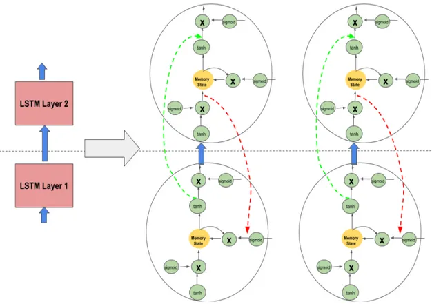
Next, the recurrent layer connectivity was fixed and neuroevolution was applied to discover new gated recurrent node architectures. The gated recurrent node can be represented as a tree. While, a LSTM node has a carefully designed gating logic, in this experiment, evolution was tasked to search for a better gating mechanism. A single LSTM node, when represented as a tree, can be considered as a five layer deep network (see Figure 2.2). Evolution enables search for deeper and larger gated recurrent nodes. Thus, the search space for node evolution is orders of magnitude larger than layer evolution. Sopshisticated neuroevolution techniques are needed to search such a large architectural space. A combined ge-netic programming and NEAT (called NEAT) is used for this purpose. GP-NEAT combines the best ideas from genetic programming (for e.g. structural tree distance and homologous crossover) with the advantages of NEAT (for e.g. speci-ation). New techniques are proposed in this dissertation to exhaustively compare tree structures and deduce their similarity, thus avoiding redundant trees in the population. Additionally, there were three key innovations that were developed in this dissertation for evolving gated recurrent nodes.

First, a new mechanism to encourage exploration of architectures was de-vised. An archive of already-explored areas (called Hall of Shame) is maintained during the course of evolution. This archive is used to drive architecture search towards new un-explored regions. The effect is similar to that of novelty search ( Lehman (2012)), but does not require a separate novelty objective, simplifying the search.

Second, experiments were conducted to show that evolution of neural net-work architectures in general can be speeded up significantly by using an LSTM network to predict the performance of candidate neural networks. After training the candidate for a few epochs, such a Meta-LSTM network predicts what

(15)

per-formance a fully trained network would have. That prediction can then be used as fitness for the candidate, speeding up evolution fourfold in these experiments. While network performance prediction has recently gained some attention ( Baker et al. (2017)), this is the first study that actually deploys fitness prediction mecha-nism to discover new and significantly improved gated recurrent architectures.

Third, taking inspiration from the results of layer evolution, where a new feedback connection led to performance improvement, an extra recurrent connec-tion is introduced within the node. Evoluconnec-tion is tasked with finding the appopriate gating logic within the recurrent node. Combining all these innovations speeds up evolution, resulting in the discovery a of new gated recurrent node that outper-forms LSTMs and other state-of-the-art recurrent nodes like NAS ( Zoph and Le (2016)) and RHN ( Zilly et al. (2016)) in the language-modeling domain (See Fig-ure 5.9).

Finally, the results from evolution were transfered to the music domain. Here, the best evolved recurrent node was used for polyphonic music generation. The data set used for training and evaluation consists of classical piano tunes. In-terestingly, in this domain, the evolved nodes were outperformed by the LSTMs. This suggest that evolution discovered a recurrent architecture customized for the language-modeling problem. An interactive music generation application was cre-ated that takes a few input notes from the user and then uses the gcre-ated recurrent networks to automatically compose a new musical piece.

1.4

Guide to the Reader

Chapter 2 describes the concepts used across this dissertation. It also dis-cusses previous work in gated recurrent network architecture search. Chapter 3 looks at RL based memory problems and proposes solutions to solve them using evolved LSTMs. Gated recurrent networks are evolved for supervised learning in Chapter 4 and 5. In chapter 4, the connectivity between two LSTM layer is evolved. Chapter 5 looks at evolving gated recurrent nodes while keeping the layer connectivity fixed. In Chapter 6, the best evolved solution from Chapter 5 is transfered to the music domain. This chapter also includes details about an application created to compose music using recurrent networks. Chapter 7 lists

(16)

possible future direction for this research. The contributions of this research and conclusions are provided in Chapter 8.

(17)

Chapter 2

Background and Related Work

Recurrent Neural Networks are generative models that produce outputs which can be used as inputs in future time steps. The experiments performed in this work demonstrate how to build such memory networks for RL and su-pervised learning tasks. The challenges in these two kinds of problems are dif-ferent. This chapter provides detail on the concepts used across the dissertation. For e.g. RNNs, LSTMs and their applications. Recently, techniques like regular-ization, batch normalization and architecture modifications have been proposed to improve the performance of LSTMs on supervised learning tasks. Since the LSTM networks for RL problems are much smaller than the ones used for super-vised tasks, these techniques do not yield as much performance improvements. RL problems come with their own set of challenges like deceptive rewards.

This chapter also briefly describes the existing neuroevolution technologies that are extended for LSTM evolution in later chapters. RL tasks in deep T-maze are used for evaluation in Chapter 3 and language and music tasks are used for supervised learning in subsequent chapters.

2.1

Vanishing Gradients in Recurrent Neural Networks

One major limitation of RNNs is that they are not able to maintain contexts for longer time sequences. This occurs because of two reasons. First, the memory state of a RNN keeps getting updated at each time step with new feedforward inputs. This means that the network does not have the control of what and how much context to maintain over time. This behavior negatively effects RNNs even when their weights are trained with gradient-free methods like evolution. Second, when RNNs are trained with backpropagation through time, they are not able to properly assign gradients to previous time steps due to squashing non-linearities. This is called as the vanishing gradient problem.

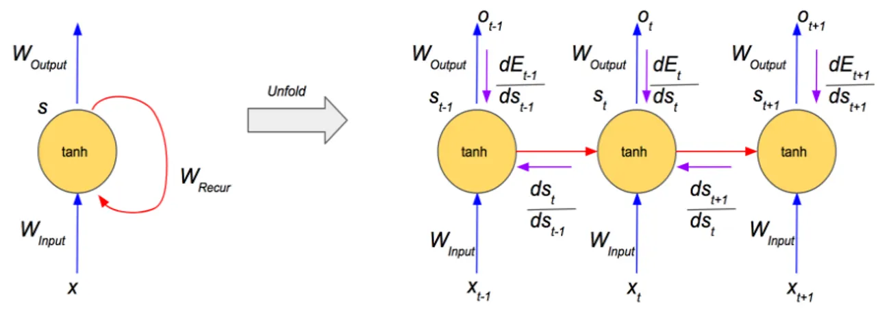
As shown in Figure 2.1, the gradient flows back through time in the unrolled RNN. Equation 2.1 describe the feedforward activation in each step of the RNN. Equation 2.2 and 2.3 describe the error that is backpropagated from time stept+ 1

(18)

Figure 2.1: Gradient flow in RNNs: on the left is a simple RNN and on the right is its unrolled version. Purple arrows depict gradient flow back in time.

to the time stept−1. Since the derivative oftanhis bounded between 0 and 1, the gradient can vanish during backpropagation (Pascanu et al. (2013) This vanishing gradient problem leads to poor performance of RNNs in deep sequential tasks.

st=tanh(Winputxt+Wrecurst−1+b) (2.1)

∂Et+1 ∂st−1 = ∂Et+1 ∂st+1 ∂st+1 ∂st ∂st ∂st−1 (2.2) ∂st ∂sk = t Y k+1 ∂si ∂si−1 = t Y k+1

Wrecurdiag(tanh0(si−1)) (2.3)

2.2

LSTM

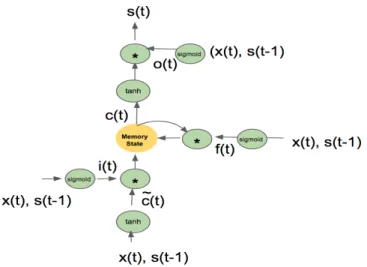
LSTMs were designed to overcome the vanishing gradient problem by con-trolling gradient flow using extra control logic and by providing extra linear path-ways to transfer gradient without squashing Hochreiter and Schmidhuber (1997b). LSTM include three types of control gates: write control that determines the input to the memory state (with linear activation), forget gate that controls how much of the stored memory value is transferred to the next time step, and output gate which regulates the output of the memory cell. In addition, LSTM units can in-clude extra peephole connections to probe the internal memory state. The

(19)

peep-hole connections allow the LSTM gates to be modulated based on value stored in the internal memory state. The output activation function is tanh. Structure of a single LSTM unit is depicted in Figure 2.2. Equations 2.4, 2.5, 2.6, 2.7, 2.8, 2.9 are the for the feedforward path. During backpropagation, the gradient for _∂s∂st

k

still goes through a couple oftanhnon-linearities. However, there is an additional linear pathway through memory cell ct that preserves the gradient based on the

control logic. Gated Recurrent Unit (GRU) is a variant LSTM in which the input and forget gates are merged for effeciency. Thus, gated recurrent networks outper-form RNNs in long sequence processing task and are therefore applicable in many domains.

it =σ(Winputixt+Wrecurist−1+bi) (2.4)

˜

ct=tanh(Winputcxt+Wrecurcst−1 +bc) (2.5)

ft=σ(Winputfxt+Wrecurfst−1+bf) (2.6) ot =σ(Winputoxt+Wrecurost−1+bo) (2.7) ct=ct−1∗ft+ ˜ct∗it (2.8) st=tanh(ct)∗ot (2.9) ∂ct ∂ct−1 =ft (2.10) ∂ct ∂ck = t Y i=k+1 ∂ci ∂ci−1 = t Y i=k+1 fi (2.11) ∂E ∂it = ∂E ∂ct ∂ct ∂it = ∂E ∂ct ˜ ct (2.12) ∂E ∂ft = ∂E ∂ct ∂ct ∂ft = ∂E ∂ct ct−1 (2.13) ∂E ∂c˜t = ∂E ∂ct ∂ct ∂c˜t = ∂E ∂ct it (2.14) ∂E ∂ct−1 = ∂E ∂ct ∂ct ∂ct−1 = ∂E ∂ct ft (2.15)

(20)

Figure 2.2: LSTM node architecture: LSTM include three types of control gates: write control that determines the input to the memory state (with linear activation), forget gate that controls how much of the stored memory value is transferred to the next time step, and output gate which regulates the output of the memory cell. For backpropagation, LSTM node is unrolled in time similar to RNN.

2.3

Applications of LSTMs

Gated recurrent networks like LSTMs and GRUs have made many real-world sequence processing applications possible, in particular those that include supervised training with time-series data. For e.g. they are widely used for su-pervised sequence learning problems like machine translation ( Bahdanau et al. (2015a)), image captioning ( Vinyals et al. (2015)), web traffic forecasting ( Suilin (2017)), speech recognition ( Bahdanau et al. (2015a)), handwriting recognition, automatic music transcription ( Ycart and Benetos (2017)), sentiment analysis and stock market prediction.

Converting a sentence from English to French is an example of a Machine translation problem. Sequence-to-sequence LSTM models are often used for this purpose Sutskever et al. (2014). They consist of two parts: an encoder and a de-coder. The input sentence is fed into the encoder one word at a time. The decoder outputs a sequence of words in the target language. The encoder outputs are ig-nored while the decoder outputs are used to compute the network loss. The ad-vantage of such sequence to sequence model is that they are effective even when the input and output sequences are of varying length. One such encoder-decoder

(21)

model is used in this work for network learning curve prediction (see Section 5.7). Image captioning is an example of LSTMs being used as a generative model. Given an input image, the goal is to generate a sequence of words describing that image. The model often consists of a convolutional network to process the im-age followed by a layer of LSTM. The LSTM layer functions as a type of languim-age model that takes the image embeddings in its first time-step and generates a se-quence of words in the subsequent time-steps (see Section 2.7.1 for more details on the language model).

Problems like speech and hand-writing recognition often use bi-directional LSTM Schuster and Paliwal (1997). Bi-directional LSTM process the data in both directions with two separate hidden layers, which are then fed forwards to the same output layer Graves and Jaitly ((2014).

LSTMs can also used be used for classification tasks like sentiment analysis. A set of text articles, tweets or reviews can be fed into the LSTM and the hidden value activation (st) of the final layer at the last time-step can be treated as an

embedding for the whole article. This embedding can then be used to predict the sentiment of the article.

2.3.1

LSTMs for Reinforcement Learning problems

Although LSTMs are commonly used in supervised tasks, they can be used in RL as well, as both policy controller and function approximator. For exam-ple, LSTM based network was used as a function approximator in the robot nav-igation task Bakker et al. (2003). In this work, the input sequence to LSTM was pre-processed to capture salient information from the environment. An unsuper-vised event extraction was performed by classifying stream of inputs into a vari-able number of distinct classes. Any change in input stream class is considered an event, and is fed into a RL model consisting of LSTM function approximator. One drawback of this method is that it can ignore sequential information that re-mains fixed during a trial but changes across trials. Wierstra et al. ((2010) applied policy gradient algorithm to train LSTM networks resulting in deeper memories for POMDP tasks. LSTM layers can be combined with Deep Q-Network (DQN) to integrate information over time and perform better in Atari games Hausknecht and Stone (2017). LSTMs can be trained through policy gradient algorithm to solve

(22)

meta-learning problems like network achitecture search Zoph and Le (2016) and learning new learning rules for gradient descent Andrychowicz et al. (2016).

Bayer et al.Bayer et al. (2009a) evolved custom LSTM memory cells using mutation operators. These custom cells are then manually instantiated to construct LSTM network for solving the T-maze problem. Their result suggests that evolving LSTMs can lead to interesting solutions to POMPD problems that are difficult to solve otherwise. Yet the evolved memory is not deep enough to be useful in real-world AI tasks (like deep T-maze or modeling hyena emotions). New methods are required to scale the evolution of LSTM to such tasks. Powerful neuroevolutionary techniques (like NEAT) is one candidate approach to achieve complex memory solutions. NEAT can evolve both the topology and weights of a LSTM network in a non-parametric manner. Chapter 3 describes one such approach of evolvng LSTMs for RL.

2.4

Improvements in LSTMs

In recent past, several techniques have been developed to improve the per-formance of LSTMs. For e.g. weight regularization, activation regularization, dropouts, modifed stochastic gradient descent, variable length back propagation through time and new recurrent node and network architectures. Such variations are usually developed] on supervised learning problems like language modeling but can be extended to reinforcement learning domain. These improvements are often independent and combining them gives additive gain in performance. The following sections describe such improvements in detail.

2.4.1

Regularization

Regularization is a widely used machine learning technique to prevent the overfitting of model to the training data. It is only applied during training and not during inference. There are several ways to regularize neural network models. The traditional approaches for regularization include adding L1 and L2 weight penalty to the network loss function. For e.g when used in logistic regression,L1

penalty leads to sparse connectivity andL2penalty leads to smaller weight values. Regularization through dropout in deep networks is a more recent advancement

(23)

and leads to better generarlization. In this method, a randomly selected subset of neurons are excluded from participating in the forward and backward pass. The model is forced to work even in the absence of dropped neurons and thus creates an ensemble effect and more robust model.

Initial experiments in applying standard feedforward dropouts to recurrent networks showed degradation in performance. Zaremba et al. (2014) proposed not dropping recurrent connections (Wrecur in Figure 2.1) and applying dropouts

only to feedforward paths (termed as vanilla recurrent dropout). Later, Gal and Gharamani (2015) showed that recurrent connections can be dropped but the same dropout mask should be applied across time steps within a sequence (termed as variational recurrent dropout). They also showed applying the same principle to input sequence dropout further improves generalization. Another approach is to limit updates to LSTM’s hidden state by dropping out updates to control gates instead of the hidden unit themselves Semeniuta et al. (2016).

Smaller models often generalize better. To take advantage of this fact, Press and Wolf (2016) showed that for a language model, sharing input embedding with output weights reduces overall parameter count and makes it easier to train even larger models.

Another form of regularization modifies the hidden unit activations includ-ing a technique called recurrent batch normalization ( Cooijmans et al. (2016)). Here, the hidden unit activations are whitened by scaling them to have zero mean and unit variance. The model activations thus stay in linear range of non-linearities liketanhand thus prevent vanishing gradients.

Experiments in Chapter 3 do not use any regularization since the models are relatively small. Layer evolution (Chapter 4) uses vanilla dropouts as pro-posed in Zaremba et al. (2014) and node evolution (Chapter 5) uses variational dropouts ( Gal and Gharamani (2015)), L2 weight regularization and shared em-beddings( Press and Wolf (2016)).

2.4.2

Improvements through Architecture Modifications

Experiments in feedforward networks have previously indicated that archi-tecture matters. Recent work suggests that the same could be true for recurrent networks. Grid-LSTMs ( Kalchbrenner et al. (2015)) and gated feedback recurrent

(24)

networks ( Chung et al. (2015)) are examples of LSTM variants with modified layer connectivity. Zilly et al. (2016) came up with a new kind of recurrent node called the recurrent highway network. It consists of a 10-layer deep network within each recurrent node. The internals of the weights are trained during backpropagation (unlike LSTM node where internal weights are fixed to 1.0).

Automatic design of networks is an emerging area of research and often described as meta-learning. The ’meta’ algorithm could be either a reinforcement learning algorithm, evolutionary algorithm or a recurrent network itself.

Initial work in discovering new recurrent architectures did not yield promis-ing results ( Klaus et al. (2014)). However, a recent paper from Zoph and Le (2016) showed that policy gradients can be used to train a LSTM network to find better LSTM designs. In Zoph and Le (2016), a recurrent neural network (RNN) was used to generate neural network architectures, and the RNN was trained with re-inforcement learning to maximize the expected accuracy on a learning task. This method uses distributed training and asynchronous parameter updates with 800 graphic processing units (GPUs) to accelerate the reinforcement learning process. Baker et al., (2017) have proposed a meta-modeling approach based on reinforce-ment learning to produce CNN architectures. A Q-learning agent explores and exploits a space of model architectures with an−greedy strategy and experience replay. These approaches adopt the indirect coding scheme for the network repre-sentation, which optimizes generative rules for network architectures such as the RNN. Suganuma et al. (2017) propose a direct coding approach based on Cartesian genetic programming to design the CNN architectures.

2.5

Evolutionary Techniques - Genetic Programming, NEAT

Evolutionary algorithms fall into the category of gradient-free global search techniques that are very effective for solving non-differentiable problems or prob-lems with very weak gradient information. For e.g. in reinforcement learning do-main, evolutionary algorithms like NEAT are quite competitive with Q-learning and policy gradient methods ( Stanley et al. (2003)). With the advent of deep learn-ing, the policy gradient methods have made a comeback. REINFORCE trick allows a non-differentiable reward to be converted into a differentiable surrogate that can

(25)

be used as an objective to train the policy neural network using stochastic gradient ascent ( Williams (1992)). One advantage of NEAT is that unlike policy gradient that only trains weights, NEAT can be used to evolve both the structure and the weights simultaneously.

Genetic Programming (GP) is another evolutionary technique that modifies tree structure instead of graphs (as in NEAT). Both NEAT and GP have variable length genotype encoding. The following two sub-section describe NEAT and GP in more detail.

2.5.1

NEAT

NEAT is a neuroevolution method that has been successful in solving se-quential decision making tasks (Stanley and Miikkulainen (2002; 2004), Lehman and Miikkulainen (2014)). When used for RL, the evolved network is used as a policy controller that receives sensory inputs and outputs agent actions at each time step. NEAT begins evolution with a population of simple networks and gradually modifies the network topology into diverse species over generations. As new genes are added through mutations, they are assigned unique historical markings called innovation number. During crossover, genes with the same histor-ical markings are recombined to produce offsprings. The population of networks is divided into different species based on number of shared historical markings. Speciation protects structural innovations in networks and maintains diversity by reducing competition among different species. The historical markings and specia-tion thus allow NEAT to construct complex task-relevant features. Memory can be introduced into the network by adding recurrent connections through mutations. NEAT is an ideal choice to evolve networks with memory in a non-parametric manner.

In Chapter 3, NEAT is used to evolve both the structure and weights of a LSTM policy controller network. In Chatper 4, a simplified version of NEAT with no speciation and crossover is used to evolve connectivity between two LSTM layers. NEAT is combined with GP to evolve gated recurrent nodes in Chapter 5.

(26)

2.5.2

Genetic Programming

Genetic Programming (GP) is an Evolutionary Computation technique that builds solutions represented as expresssions/programs. Similar to NEAT, it can start from a simple expression that eventually grows over time. At the start of evo-lution, a population of randomly generated simple expressions are evaluated. Ge-netic programming iteratively transforms a population of parent expressions into a new generation of the offspring by applying genetic operations like crossover and mutations. These operations are applied to individual(s) selected from the popu-lation. The individuals are probabilistically selected to participate in the genetic operations based on their fitness.

The expression in the tree is often represented as a tree with left and right branches. For e.g. in Chapter 5, the gated recurret node is represented as a tree and therefore can evolved using GP. A variant of GP, called cartesian genetic pro-gramming, allows evolution of graphs as well ( Suganuma et al. (2017)).

One of the challenges in scaling GP is that it can suffer from bloating i.e. programs can grow unnecessarily large without fitness improvements. To over-come this problem, the idea of diversity maintenance through speciation in NEAT can be combined with GP ( Tujillo et al. (2015)).

2.6

Diversity in Evolution

Fitness landscape in many high-dimensional problems is deceptive that can lead to local optima. When evolving topologies of the network, this effect can lead to bloating Tujillo et al. (2015). Speciation in NEAT addresses this problem by maintaining different kinds of networks in the population. The same ideas can applied to genetic programming (as shown in Chapter 5).

Diversity can be used to characterize the behavior of the network in RL or in supervised learning domains. For e.g. the set of actions that the agent takes within an episode could be its behavioral vector and the agent’s behavioral novelty can be measured in terms of the vector distance from agents’ actions ( Lehman (2012)). In the supervised problem like language modeling defining network diversity is more compute intensive because of the presence of vastly more data points. There-fore, diversity of network structure is often measured and maximized. Novelty

(27)

search is one such objective that can applied to either maximize behavioral or struc-tural diversity. Howerver, it converts the problem into multi-objective problem. In Chapter 5, structure diversity of recurrent nodes is maximized using a Hall of Shame. This includes keeping a fixed size archive of already explored regions in the architectural search space and preventing reproduction from spawning indi-viduals in those areas. Thus, we can induce structural novelty without explicitly maximizing it.

For RL problems, the problem of deception is more pronounced due to sparser rewards. For e.g. in a maze search problem, where a small reward can be found at a nearby corner from the agent and a high reward placed far away, the agent learns to greedily act and settle for smaller reward. To overcome this, Chap-ter 3 presents a new information maximization objective that motivates the agent to explore areas that provides new information. The information maximization objective quanitfies the novetly of information in terms of entropy. This additional objective is closely aligned with NEAT such that the evolved networks have max-imial information stored in LSTM nodes in the most efficient way possible.

2.7

Problem Domains

Three benchmark problems are used to evaluate the technology developed in this work. Deep T-maze is a RL problem used in Chapter 3. Chapter 4 and 5 use language modeling as a benchmark problem. The solution evolved in Chapter 5 for language modeling is then transfered to music data.

2.7.1

Language

The goal of language modeling is to estimate the probability distribution of wordsP(w)in a English language sentence.

This has application in speech recognition ( Graves and Jaitly ((2014)) and machine translation( Bahdanau et al. (2015b)) and text summarization. Training better language models (LM) improves the underlying metrics of the downstream task (such as word error rate for speech recognition, or BLEU score for transla-tion), which makes the task of training better LMs valuable by itself. Further, when trained on vast amounts of data, language models compactly extract knowledge

(28)

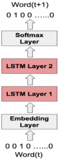
Figure 2.3: LSTM based Neural Network Language Model. Words are encoded as one-hot vectors and fed into a embedding layer. Two LSTM layers are stacked on top of the embedding layer and the final layer is softmax. The network outputs word probabilities for the next word in the sentence. In this manner, the network can be used for next word prediction.

encoded in the training data. For example, when trained on movie subtitles, these language models are able to generate basic answers to questions about object col-ors, facts about people, etc. ( Józefowicz et al. (2016))

Statistical language models have been previously used where the model learns probability of word occurrence based on examples of text. Bi-grams and tri-grams are examples of such N-gram models where word transition probabilities are computed by counting frequency of co-occurence of words in the training data. Such models are simple to design and work well for short sentences but are not powerful enough to capture dependencies in longer sentences.

Recently, the use of neural networks in the development of language models has become very popular, to the point that it may now be the preferred approach. Nonlinear neural network models solve some of the shortcomings of traditional language models: they allow conditioning on increasingly large context sizes with only a linear increase in the number of parameters, they alleviate the need for manually designing backoff orders, and they support generalization across differ-ent contexts.. Figure 2.3 shows example of one such LSTM model. In every time step, the model takes in a one hot encoded word as input. A linear embedding

(29)

layer converts the discrete word input into a real-valued vector to represent each word in the projection space. A stack of two LSTM layers combine the word em-bedding with the context stored in their memory. Finally the softmax layer outputs word probabilities. Such a model can be trained using stochastic gradient descent (SGD).

Recurrent Neural Networks based LMs employ the chain rule to model joint probabilities over word sequences:

p(w1, w2, ...wn) = N

Y

i=1

p(wi|w1, w2...wi−1) (2.16)

where the context of all previous words is encoded with an LSTM, and the probability over words uses a Softmax (see Figure 2.3).

A good language model is one which assigns higher probability to gram-matically correct or frequently observed sentences than ungrammatical or rare ones. One metric to measure this performance is called word perplexity.

P erplexity(w1, w2, ...wn) = P(w1, w2, ...wn)

−1

n (2.17)

P erplexity(wi) = exp(Average Cross Entropy Loss per W ord) (2.18)

Average Cross Entropy Loss per W ord=

N−1

X

i=0

−Pitargetlog(Pipredicted) (2.19)

A completely random model that assigns every word in the sentence equal probability (p= _N1, whereN is the vocabulary size) will have perplexity ofN. This is the worst case performance of the model. Thus, a model with lower perplexity value on the test data is considered better.

In this word, the experiments are focused on the task of predicting the next word in the Penn Tree Bank corpus (PTB), a well-known benchmark for language modeling Marcus et al. (1993). LSTM architectures in general tend to do well in this task, and improving them is difficult Zaremba et al. (2014) Jozefowicz et al.

(30)

(2015) Gal and Gharamani (2015). The dataset consists of 929k training words, 73k validation words, and 82k test words, with a vocabulary of 10k words. During training, successive minibatches of size 20 are used to traverse the training set sequentially.

2.7.2

Music

Music consists of a sequence of notes that often exhibit temporal depen-dence. Predicting future notes based on the previous notes can therefore be treated as a sequence prediction problem. Similar to natural language, musical struc-ture can be capstruc-tured using a music language model (MLM). Just like natural lan-guage models form an important component of speech recognition systems, poly-phonic music language model are an integral part of Automatic music transcrip-tion (AMT). AMT is defined as the problem of extracting a symbolic representa-tion from music signals, usually in the form of a time-pitch representarepresenta-tion called piano-roll, or in a MIDI-like representation. Despite being one of the most widely discussed topics in music information retrieval (MIR), it remains an open problem, in particular in the case of polyphonic music (Lewandowski et al. ((2012), Lavrenko and Pickens (2003.))..

MLM predict the probability distribution of the notes in the next time step. Multiple notes can be turned-on at a given time step for playing chords. The archi-tecture of MLM is very similar to the one shown in Figure 2.3. One key difference is that the output layer in case of MLM consists of a sigmoid layer (for chords). The loss function used for training the network is cross-entropy between predicted note and the target notes (see equation 2.19). The metric used to evaluate MLM is called the F-measure. F-measure is computed on the test data by taking the geo-metric mean of precision and recall.

The input is a piano-roll representation, in the form of an 88XT matrix M, where T is the number of timesteps, and 88 corresponds to the number of keys on a piano, between MIDI notes A0 and C8. M is binary, such that M[p, t] = 1

if and only if the pitch p is active at the timestept. In particular, held notes and repeated notes are not differentiated. The output is of the same form, except it only hasT1timesteps (the first timestep cannot be predicted since there is no previous information).

(31)

Piano-midi.de dataset is used as the benchmark data. This dataset currently holds 307 pieces of classical piano music from various composers. It was made by manually editing the velocities and the tempo curve of quantised MIDI files in order to give them a natural interpretation and feeling ( Ycart and Benetos (2017)).. MIDI files encode explicit timing, pitch, velocity and instrumental information of the musical score.

2.7.3

RL Memory Tasks

Most real-world RL applications are POMDPs and require some form of recurrency to solve the problem of state aliasing. In order to sucessfully solve such problems, a combination of sophisticated RL algorithm and simple memory architecture is required. For e.g. in the atari video game, while the overall agent performance improves with the addition of an LSTM layer, the same improvement can be achieved by feeding multiple consecutive frames to a feedforward network ( Hausknecht and Stone (2017)). Since the goal of experiments in Chapter 3 is to solve deep memory problems, a customized task is designed for this purpose called deep T-maze.

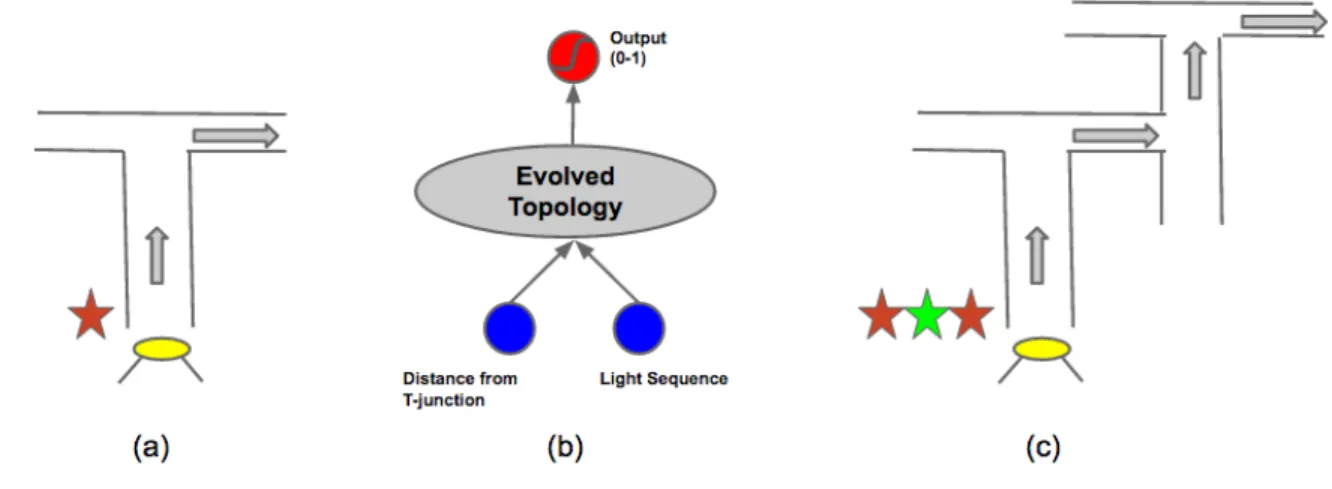
Standard T-mazes are widely used as testbed for RL problems. At the be-ginning of each trial, the agent observes one light. As the agent moves forward in the aisle towards the T-junction, it no longer has access to the light. The color of the light (red/green) indicates the direction (right/left) that the agent should take at T-junction in order to reach the goal. Therefore, to be successful, the agent needs to memorize the color of the light that was shown at the start. The problem of T-maze can be easily scaled to a Deep T-maze. In this case, there are multiple input lights at the start corresponding to the multiple T-junctions. In order to be successful, the agent is required to recall the input light sequence in the correct order at each T-junction. This task requires deeper memory than the simple T-maze (See Figure 3.2 for details).

(32)

Chapter 3

Evolving LSTM Network Structure and Weights using

Unsupervised Objective - InfoMax

In this chapter, NEAT (Neuroevolution of Augmenting Topologies) Stanley and Miikkulainen (2002) algorithm is extended to incorporate LSTM nodes (NEAT-LSTM). Since NEAT algorithm can evolve network topologies, it can discover the correct amount of memory units for the task. NEAT-LSTM outperform RNNs in two distinct memory tasks. However, NEAT-LSTM solutions do not scale as the memory requirement of the task increases. To overcome this problem, a secondary objective is used that maximizes the information stored in the LSTM units. The LSTM network is first evolved during the pre-training phase with this unsuper-vised objective to capture and store relevant features from the environment. Sub-sequently, during the task fitness optimization phase, the stored LSTM features are utilized to solve the memory task. This approach yields LSTM networks that are able to solve deeper memory problems. Two memory tasks are used to compare the performance of different algorithms: sequence recall and sequence classifica-tion.

3.1

Problem of Deception

From an optimization perspective, since the problem of evolving memory is deceptive, extra objectives (to promote solution diversity) can be used to over-come deception Lehman and Miikkulainen (2014), Ollion et al. (2012). In such ap-proaches, the evolutionary optimization problem is often cast as a multi-objective problem with two objectives - primary objective (task fitness) and secondary di-verstiy objective (like novelty search). However, there are no guarantees that such diversity objectives can aid the learning algorithm to capture and store useful his-torical information from the environment. Since the secondary diversity objective is unrelated to the task fitness, the network can also undergo unsupervised pre-training to optimize this objective. One such unsupervised objective is presented in this dissertation that maximizes the total theoretic information stored in the LSTM

(33)

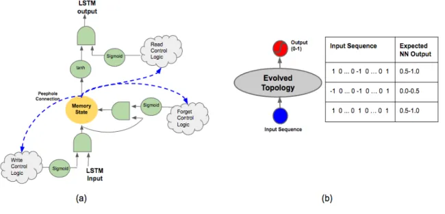
Figure 3.1: (a) The LSTM node with peephole connection: a single LSTM unit is comprised of three components: (1) green-colored multiplication gates and sig-moid/tanh activation function, (2) yellow-colored internal memory state with lin-ear activation, and (3) blue-colored peephole connections. There are three multi-plication gates (write, forget and read) that control the flow of information through the LSTM unit. The peephole connections allow the internal memory state of the LSTM unit to be probed. The peripheral control logic (shown in gray cloud-shaped boxes) and the peephole connection weights are modified during the course of evolution. (b) The Sequence-Classification Task: This is a binary classification task where the network has to count whether the number of 1s in the input se-quence exceeds the number of -1s (0s are ignored). At the start of evolution, the network consists of one input node and one output node. NEAT evolves hidden layer topology. A network requires memory in order to succeed in this task. Ex-ample of input-output sequence values are shown in the table.

(34)

network.

3.2

Unsupervised Training of LSTM

In supervised learning domain, unsupervised pre-training of neural net-works to initialize its parameters has been shown to improve the overall network task performance significantly. This idea of pre-training the network with unsu-pervised objective can also be extended to the RL domain. However, not much literature exists on the topic of unsupervised pre-training of LSTM for RL POMDP tasks. On a related note, Klapper-Rybicka et al. (2001) performed unsupervised clustering of musical data using LSTM networks. In this work, Binary Informa-tion Gain OptimizaInforma-tion (BINGO, Schraudolph and Sejnowski (1993)) was used as an unsupervised objective. BINGO maximizes the information gained from ob-serving the output of a single layer network of logistic nodes, interpreting their activity as stochastic binary variables. One limitation of BINGO is that it searches only for uncorrelated binary features (thus the solution ends up having zeros and ones in equal parts), which limits the amount of information the network can store. Instead, LSTM features with maximal information are evolved in this work. Specif-ically, the LSTM networks are evolved (using NEAT) to first extract and store in-dependent (and highly informative) real-valued features. These features are then later used to solve the memory task. Storing independent features in the LSTM en-sures that the network has maximal information from a theoretic perspective. This information-theoretic objective to train LSTM network is similar to the info-max approach published in Bell and Sejnowski (1995). However, the main difference is that there is no underlying assumption on the number of mixed features and the linearity of the mixture.

3.3

Memory Tasks

This section describes two memory tasks. Both the tasks are situated in a discrete maze where the agent moves one-step at each time-step of the trial. The first task, sequence classification, is a binary classification problem of streaming input. The second task, sequence recall, requires the agent to recall a previously

(35)

Figure 3.2: (a) Sequence Recall in simple T-maze: At the beginning of each trial, the agent observes one light. As the agent moves forward in the aisle towards the T-junction, it no longer has access to the light. The color of the light (red/green) indicates the direction (right/left) that the agent should take at T-junction in order to reach the goal. Therefore, to be successful, the agent needs to memorize the color of the light that was shown at the start. (b) Network architecture: In this task, the network has two inputs: one input represents the distance to the T-junction and the second input is the light sequence (active only during the first few time steps) (c) Deep T-maze: In the Deep T-maze, there are multiple input lights at the start corresponding to the multiple T-junctions. In order to be successful, the agent is required to recall the input light sequence in the correct order at each T-junction. This task requires deeper memory than the simple T-maze.

(36)

provided instruction input and use it to make future decisions (turn left or right at the T-junction). In both the tasks, the agent is required to store and to utilize the past events in order to be successful in the task.

3.3.1

Sequence Classification

This is a binary classification task, where given an input sequence of 1 and -1 (interleaved with 0s), the network needs to determine whether it received more 1s than -1s. The number of interleaved 0s in the input sequence is random and ranges between (10-20 time steps) . This task can be visualized as a maze positioning task. An agent situated at the center of a one-dimensional maze is provided instructions to move either left/right. It is expected to move left (west) when its input is -1 and move right (east) when its input is 1. When its input is zero, it is not expected to move. At the end of the sequence, the agent needs to identify whether it is on the right side of the maze or the left side i.e. has it taken mores steps towards east than west. Note, that input 0 does not affect this decision but only serves to confuse the agent. The number of turns (left/right) that the agent takes during a trial is defined as the depth of the task. For example, a sequence of four turns (total four 1/-1 inputs interleaved with 0 in the input sequence) is termed as 4-deep. Different sequence classification experiments are carried out by varying the depth of the task (4/5/6 deep). The network architecture and example input-output combinations are shown in Figure 3.1b.

3.3.2

Sequence Recall

In the simple T-Maze, at the beginning, an agent receives an instruction stimulus (like red/green light) (see Figure 3.2a). The agent then travel a corridor until it reaches the T-junction. At the junction, the path splits into two branches (left/right) and the agent needs to take the correct branch in order to reach the reward. The position of the reward is indicated by the instruction stimulus it re-ceived at the beginning. For example, red light can indicate presence of reward on the right-branch and green light can indicate the reward on left branch. A suc-cessful agent thus can only maximize collecting the reward by memorizing and utilizing its stimulus instruction. T-Maze has been widely used as a benchmark

(37)

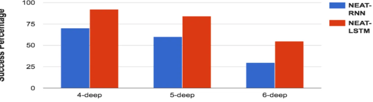
Figure 3.3: NEAT-LSTM vs. NEAT-RNN comparison on the Sequence-Classification task. The memory depth requirement is varied on the x-axis. The y-axis values represents the success rate of each method in 50 runs. The perfor-mance of NEAT-RNN and NEAT-LSTM is comparable for 4-deep sequence classifi-cation. As the task depth is increased to 6-deep, NEAT-LSTM significantly outper-forms NEAT-RNN. Successful solutions to the sequence-classification task should be able to retain an aggregate of previous inputs and should also continuously update this aggregate with new incoming inputs. The performance results indi-cate that LSTM-based networks can memorize information over longer intervals of time as compared to RNNs.

(38)

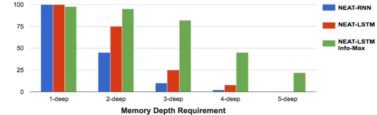
Figure 3.4: NEAT-LSTM, NEAT-RNN and NEAT-LSTM Info-max comparisons on Sequence-Recall task. Success percentage of each method is plotted for T-maze with varying depth. Both NEAT-RNN and NEAT-LSTM can quickly find the solu-tion to simple one-step T-maze. As the maze becomes deeper, NEAT-LSTM outper-forms NEAT-RNN. However, beyond 3-deep, the problem becomes too complex for both the methods. A solution to the deep T-maze problem requires memo-rizing the input light sequence in its correct order for several hundred time-step. NEAT-LSTM Info-max can successfully find solutions for even 5-deep recall. This suggests that pre-training of LSTM networks with unsupervised Info-max objec-tive results in the capture of useful information from the environment that can later be used to solve the memory task.

problem for evaluating agents with memory Bakker (2002), Bayer et al. (2009a), Lehman and Miikkulainen (2014), Ollion et al. (2012).

This simple T-maze (with one T-junction) can then be extended to a more complex deep T-maze which consists of a sequence of independent T-junctions (Figure 3.2c.). Here, the agent receives a sequence of ordered instructions (one corresponding to each T-junction decision) at the start of trial and it has to utilize the correct instruction at every T-junction in order to reach the goal. Risi et al. Risi et al. (2010.) used one such T-maze extension (double T-maze) to test plastic neural networks. The distracted sequence recall task used in Monner and Reggia (2012) is another variation of the deep T-maze recall, but it uses supervised training to learn the LSTM parameters. However, the approach presented in this dissertation uses a weak fitness signal (proportional to the number of correctly recalled input instructions) to train the memory network. Scaling the memory depth of network to recall long sequences in such RL settings has been a challenge.

(39)

3.4

Experiments

The following experiments have a three goals. First, to compare the perfor-mance of RNNs vs. LSTM in the memory tasks. Since LSTMs outperform RNNs in supervised domain, the hypothesis is that they can do the same in the RL do-main as well. Second, the LSTMs based networks are scaled to deeper memory tasks to understand their bottlenecks. Finally, a new unsupervised objective called Info-Max is presented that enables deeper LSTMs.

In each experiment, a population of 100 networks is evolved using NEAT for 15,000 generations. Each individual in the population is evaluated on all possi-ble input sequences. Deeper tasks therefore require more evaluations than shallow ones. The length of each trial also depends on the task-depth. For example, a 4-deep sequence classification task consists of at least four time steps (corresponding to four 1/-1) and 40 time steps of 0 inputs interleaved between 1/-1. During evo-lution, out of a total fitness of 100, the network receives a fraction for correctly predicting a part of the problem. For example, in a 4-deep sequence classification problem, if the agent correctly predicts its position in the maze (left or right side) after two turns, then it receives 50 fitness points. It is expected that such partial reward will shape the network towards evolving optimal behavior.

Data is collected from 50 runs of each experiment type and the average suc-cess rate (percentage of runs that yield solution with maximum fitness) is mea-sured to compare performance of different methods. At each time step, the net-work under evaluation is activated once. The value at the input of a node is propa-gated to its output in a single time step. Therefore, the number of time steps it takes for the network input to reach the output is equal to the shortest path between in-put and outin-put. This setup is critical in ensuring that the network captures the input sequence values and their order correctly in the recall task.

3.4.1

Experiment 1: Comparing RNNs vs. LSTM

First, RNNs are evolved using standard NEAT algorithm (labeled as NEAT-RNN). A user-defined parameter controls the probability (set to 0.1 in these exper-iments) of adding a new recurrent link. The recurrent links can be either self-loops or a longer loop consisting of several intermediate nodes. Next, NEAT is extended

(40)

to evolve LSTM-based networks that are compared with RNNs.

Method: NEAT-LSTM

Standard NEAT algorithm can add new nodes (sigmoid or rectified linear units) through mutation. In this work, NEAT is extended such that during its search process, it can add new LSTM units (probability of adding a new LSTM unit is 0.01). On being first instantiated, LSTM gates have default values - always write, always read and always forget. This setting ensures that initially, newly added LSTM units do not affect the functionality of the existing network. Each new instantiation of a LSTM unit is associated with the corresponding addition of a minimum of six network parameters - three connections from external logic to the control gates (depicted as cloud shaped gray boxes in Figure 3.1a) and three peephole connections (blue-colored links in Figure 3.1a). During the course of evo-lution, the existing parameters can be modified/removed and new ones can be added to suit the requirements of the task. No recurrent connections are allowed except the recurrency that exists within the LSTM unit.

Results

As shown in Figure 3.3, both NEAT-RNN and NEAT-LSTM can solve the 4-deep sequence classification task easily. As memory depth requirement increases to six, their success rate gradually decreases. NEAT-LSTM significantly outper-forms NEAT-RNN in all the cases (t-test; p<0.01). The sequence-classification task is relatively simpler than the sequence-recall task. The agent is required to update and store its internal state with each new valid input (1/-1). Therefore, the success-ful networks have simple architecture (consisting of only a few recurrent neurons in the case of NEAT-RNN and a single LSTM in the case of NEAT-LSTM).

In the sequence-recall task, both NEAT-RNN and NEAT-LSTM quickly find the solution to one-step T-maze (Figure 3.4). This result is expected and it matches the outcomes of previous papers that focused on this problem (Lehman and Mi-ikkulainen (2014), Wierstra et al. ((2010)). However, as the T-maze becomes deeper, the successful solutions are required to store input light sequence information for longer durations and in its correct order. Therefore, beyond 3-deep T-maze, the

(41)

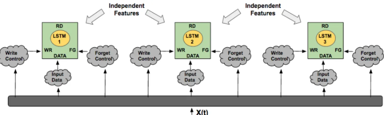
Figure 3.5: Unsupervised Pre-training using the Information Maximization objec-tive. Highly informative, independent LSTM features are incrementally added by modifying the write control, forget control and input data logic using NEAT. Unsu-pervised pre-training is carried out until evolution stops discovering independent features or at the end of 10000 generations. By the end of this pre-training phase, salient information observed by the agent is captured and stored in the LSTM net-work. The pre-training aids evolution of deeper memory solutions in two ways. First, it reduces the problem of deception by directing evolutionary search towards landscapes that provide new information. Second, by incrementally adding inde-pendent features, it avoids the problem of training a large number of LSTM pa-rameters simultaneously.

problem becomes too complex for both NEAT-RNN and NEAT-LSTM to solve.

3.4.2

Experiment 2: Scaling NEAT-LSTM

In the harder task of sequence recall, the agent needs to store the entire input sequence in correct order. Incremental evolution approach was applied in order to solve deeper recall problems (>4-deep). Networks were first evolved for 2-, 3-, and 4-deep recall problems; these networks were then used as a starting point (in the NEAT algorithm) to solve the more complex problems of increasing depth (>4-deep). However, this approach did not yield much success. The problem may be that as the length of the input sequence increases, the number of parameters to be evolved also increase (with each additional LSTM units). Also, the incremental evolution approach requires detailed knowledge of the problem domain that is not inline with the goal of this dissertation (i.e. to solve the memory task with limited domain knowledge).

(42)

Method: Information Maximization Objective

One way to overcome the problem of deception is by ensuring that evo-lution discovers unique time-dependencies by not re-discovering existing infor-mation. In solving POMDP tasks that require memory, the agent can benefit by capturing salient historical information from the environment and storing it in its neural-network controller. As the agent moves in the environment over multiple trials, it comes across a lot of information. For example, it can observe the wall (which are mostly static across trials) or it can observe a binary light (red/green in T-maze), which can provide possible clues for the location of the goal. It is difficult to discern which information should be stored for later use (blinking light) and which should be discarded (static walls).

One solution could be to store inputs (in their native form or in combination with other inputs) such that the total information stored in the network is maxi-mized. From a theoretical perspective, the information stored in a set of random variables is maximized when their joint entropy is maximized. The joint entropy of two random variablesXandYcan be defined as

H(X, Y) = H(X) +H(Y)−I(X, Y), (3.1)

H(X) = XP(X) logP(X), (3.2) whereH(X),H(Y )are the individual entropies ofXandYrespectively and I(X, Y )is the mutual information betweenXand Y. Thus, to maximize the information stored in the network, the individual entropy of its hidden unit activations should be maximized and their mutual information minimized. The mutual information can be expressed as Kullback-Leibler divergence:

I(X, Y) = XP(X, Y) log P(X, Y)

P(X)P(Y) (3.3)

Random variables with zero mutual information are statistically indepen-dent. Computing and storing highly informative, maximally independent features (i.e. features with high individual entropy and low mutual information) in the network is the unsupervised objective that will be used for NEAT (Info-max). The features are stored in the hidden LSTM units, since these units can retain

(43)

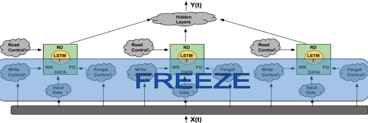
informa-Figure 3.6: RL training using the fitness objective. During the RL phase, the stored/memorized features are utilized to solve the memory task. The write con-trol, forget control and input data logic of the LSTM units (that store independent features) is frozen and the read control logic is evolved using NEAT. NEAT can add new hidden layers over the top of existing LSTM network.

tion over several time steps. Evolving independent features allows for pre-training the network and only augments the NEAT-LSTM approach as outlined in Section 4.1.1. The new learning algorithm now consists of two steps: The first one is an unsupervised objective phase where the independence of LSTM hidden units is maximized (see Figure 3.5), and the second is an RL phase where the fitness objec-tive is maximized (Figure 3.6).

A feature vector is constructed by concatenating the memory state values (yellow-colored circle in Figure 3.1) of the LSTM unit from each neural network activation across different trials. There is one distinct feature vector correspond-ing to each LSTM hidden unit. To compute entropy and mutual information, the feature vectors are treated as random variables. The real-valued features are par-titioned into 10 equal-sized bins, and a histogram is constructed by counting the number of elements in each bin. Entropy and pairwise mutual information (an ap-proximation of total mutual information) of feature histograms is then calculated using equation 3.2 and equation 3.3 respectively.

Evolving multiple independent features simultaneously can be challenging. This problem can be broken down using incremental evolution Gomez and Mi-ikkulainen (1997) (without the need for domain knowledge). Independent features (with their values stored in individual LSTM units) can be discovered one at a time

(44)

using NEAT. Since the primary goal of this work is to build networks with mem-ory, one simplifying assumption can be introduced: environment is not dynamic, i.e. it does not change over time. With this assumption, independent features once discovered and stored in LSTM need not change over a period of time. The station-arity assumption also entails that during the unsupervised training phase, only the write control logic, forget control logic and input data logic of the LSTM unit need to be modified. Once the independent features have been discovered, no more changes to the write, forget and input logic of the LSTM units are required (i.e. they are frozen). For the remainder of evolutionary search, NEAT can only add outgoing connections from the frozen network (to facilitate re-use of frozen logic). Often, there exists multiple solutions to the problem of finding networks with max-imum information. Some of these network solutions could be large. To bias NEAT towards evolving smaller solutions during unsupervised objective optimization, a regularization factor is introduced that penalizes larger networks. The size of the evolved network (equal to the number of network connections) is weighted by a regularization parameter (value varies between 0 and 1), and the resulting penalty term is subtracted from the unsupervised objective value. Unsupervised training is stopped either when NEAT cannot find any more independent features or at end of 10000 generations.

Subsequently, during the RL phase, the LSTM outputs are provided as extra inputs (in addition to the sensor inputs) to the NEAT algorithm. NEAT evolves the read control logic of the frozen LSTM units to utilize the stored features appropri-ately as deemed fit for the task. This approach makes neuroevolution computa-tionally more tractable.

Results

NEAT-LSTM with the information maximization objective (NEAT-LSTM Info-max) was evaluated on sequence-recall task, since it is the harder of the two memory tasks. As shown in Figure 3.4, NEAT-LSTM and NEAT-RNN outperform NEAT-LSTM Info-max in the 1-deep task. This is probably because NEAT-LSTM and NEAT-RNN are powerful enough to quickly find a solution to the shallow memory problem. As the memory depth requirement increases however, NEAT-LSTM Info-max consistently outperforms NEAT-NEAT-LSTM and NEAT-RNN (t-test;

(45)

p<0.01). NEAT-LSTM Info-max is able to solve 5-deep sequence recall problem about 20%of the time.

In the sequence-recall task, the networks evolved using NEAT-LSTM Info-max method can preserve information (in correct order) over hundreds of time steps. This result suggests that pre-training o