Machine Learning Methods for Fuzzy Pattern Tree Induction

(1)

Machine Learning Methods for

Fuzzy Pattern Tree Induction

Robin Senge

aus Bad Br¨uckenau

Fachbereich Mathematik und Informatik Philipps-Universit¨at Marburg

Dissertation zur Erlangung eines

Doktorgrades der Naturwissenschaften (Dr. rer. nat.) Marburg/Lahn, 2014

(2)

(3)

Vom Fachbereich Mathematik und Informatik der Philipps-Universi¨at Marburg (Hochschulkennziffer: 1180) als Dissertation angenommen am: 15.04.2014

Erstgutachter: Prof. Dr. Eyke H¨ullermeier Zweitgutachter: Prof. Dr. Christophe Marsala

weitere Mitglieder der Pr¨ufungskommission: Prof. Dr. Manfred Sommer

Prof. Dr. Bernhard Seeger

(4)

This thesis elaborates on a novel approach to fuzzy machine learning, that is, the combination of machine learning methods with mathematical tools for modeling and information processing based on fuzzy logic. More specif-ically, the thesis is devoted to so-called fuzzy pattern trees, a model class that has recently been introduced for representing dependencies between input and output variables in supervised learning tasks, such as classifi-cation and regression. Due to its hierarchical, modular structure and the use of different types of (nonlinear) aggregation operators, a fuzzy pattern tree has the ability to represent such dependencies in a very flexible and compact way, thereby offering a reasonable balance between accuracy and model transparency.

The focus of the thesis is on novel algorithms for pattern tree induction, i.e., for learning fuzzy pattern trees from observed data. In total, three new algorithms are introduced and compared to an existing method for the data-driven construction of pattern trees. While the first two algorithms are mainly geared toward an improvement of predictive accuracy, the last one focuses on efficiency aspects and seeks to make the learning process faster. The description and discussion of each algorithm is complemented with theoretical analyses and empirical studies in order to show the effectiveness of the proposed solutions.

Zusammenfassung

Diese Arbeit befasst sich mit einer neuen Methode im Bereich des “un-scharfen maschinellen Lernens”. Dieser Bereich umfasst Methoden, die eine Kombination von maschinellen Lernverfahren mit Konzepten aus der

(5)

Theorie unscharfer Mengen (Fuzzy Set Theory) darstellen. Im Speziellen beschäftigt sich die Arbeit mit der Modellklasse der sogenannten Fuzzy Pattern Trees. Diese Modellklasse wurde kürzlich vorgestellt und dient der Modellierung von Abhängigkeiten zwischen Ein- und Ausgabevariablen in Problemstellungen des überwachten Lernens (supervised learning) wie beispielsweise Regression und Klassifikation. Aufgrund ihrer hierarchischen und modularen Struktur sowie der Verwendung von unterschiedlichen, zum Teil nicht-linearen Aggregationsoperatoren ist die Modellklasse in der Lage, diese Abhängigkeiten flexibel und kompakt darzustellen. Dabei erreicht sie eine gute Balance zwischen prädiktiver Genauigkeit und Transparenz. Schwerpunkt dieser Arbeit ist die Entwicklung neuer Algorithmen zum Ler-nen von Fuzzy Pattern Trees aus Daten. Insgesamt werden in dieser Ar-beit neben einer Reihe von Heuristiken drei neue Algorithmen vorgestellt. Während die ersten beiden nahezu ausschließlich auf die Verbesserung der Prädiktionsgenauigkeit abzielen, wird mit dem dritten die Verbesserung der Laufzeit während der Trainingsphase erreicht. Die Beschreibung der Algo-rithmen ist immer sowohl von einer theoretischen Diskussion als auch einer empirischen Evaluierung begleitet, die die Effektivität und Effizienz der Al-gorithmen demonstriert und statistisch belegt.

(6)

(7)

(8)

During my PhD study, I was supported by the help of many people. Most importantly, I would like to thank my advisor Prof. Eyke H¨ullermeier. His advice and support were always very helpful and directed me to the right path for my studies. In particular, the discussions with him and his whole research group of Computational Intelligence in the Department of Math-ematics and Computer Science at the University of Marburg, were always challenging and productive. It was always fun to be part of a group, in which an environment of high-level scientific research culture exists and flourishes.

During my studies, I had the opportunity to work together with many great people. Besides Prof. Hüllermeier, I have the privilege to co-author papers with Dr. Stefan Bösner, Dr. Weiwei Cheng, Prof. Juan José del Coz, Dr. Krzysztof Dembczyński, Prof. Norbert Donner-Banzhoff, Dr. Thomas Fober, Jörg Haasenritter, Dr. Dominik Heider, Sascha Henzgen, Dr. Oliver Hirsch, Dr. Edwin Lughofer, Maryam Nasiri, Prof. Maria Rifqi and Ammar Shaker. In addition, I would like to thank Amira Abdel-Aziz for their help in revising the first versions of this thesis.

Last but not least, I would like to thank my wife Jennifer and my kids Jamila and Rodney. They not only have been a constant motivation to me to finish my studies on time, but they also reminded me that work is just a part of it all.

(9)

List of Figures

1.1 One possible formulization of a subjective perception of the fuzzy concept ”much older than 5 years”. . . 6 1.2 Example of two fuzzy numbers (top), which are combined with the

min-imum t-norm (middle) and with the maxmin-imum t-conorm (bottom). . . . 7 1.3 Example of elements existing in a 2-dimensional space, i.e. described by

two attributes (x1, x2). . . 9 2.1 An interpreted example of a fuzzy pattern tree. . . 14 2.2 The same FPT as in the previous figure with additional information

about the implementation of each node. . . 15 2.3 Example of a grid in two dimensions with two fuzzy sets for each dimension. 24 2.4 The implementation of the selector subtree S_pSel for the grid point p=

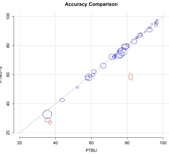
(c1, ..., c1). . . 25 2.5 The implementation of a constant function g(p). . . 25 2.6 The implementation of the function ˜g(·) using a fuzzy pattern tree. . . . 25 3.1 Algorithm by Huang, Gedeon and Nikravesh . . . 41 3.2 Creating a new candidate tree in a bottom-up manner. . . 42 3.3 Comparison of the accuracy of PTBU and PTBU-S on 40 datasets (one

ellipsoid per dataset). If both methods have the same mean accuracy, the center of the ellipsoids lay on the dashed diagonal. Ellipsoids depart from the diagonal indicate a difference in accuracy. The dimensions of the ellipsoid are determined by the standard error of the mean estimate. 49 3.4 Predictive accuracy and training runtime of PTBU-DOE for different

(12)

3.5 Predictive accuracy and training runtime of PTBU-LCH for different

values of k. Each line represents one of the 40 classification datasets. . . 53

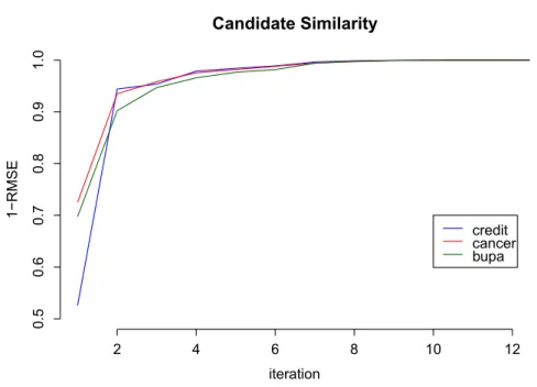
3.6 Pairwise similarity between candidate models (averaged over all pairs of candidates and over 50 random samples) for three binary datasets: credit, bupa, cancer. . . 57

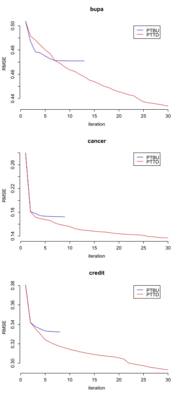
3.7 Error curve (top-down strategy in dashed, bottom-up strategy in solid line, averaged over the classes) on three datasets: bupa, cancer and credit. 58 3.8 Top-down induction: A leaf node is expanded through replacement with a three-node tree. . . 60

3.9 Top-down algorithm . . . 61

3.10 In this example, three of the six models (Box 1–3) remain in the race after this iteration. Models 4–6 can be excluded because their mean error is unlikely (< δ) to become better than the one of the current best model (Box 2). . . 69

3.11 Models compared to calculate the potential of leafL. . . 72

3.12 Result of the comparison between PTTD and PTTD-PH for different dmax values. The upper diagram shows the training time and the lower shows predictive accuracy of the methods including standard error bars. 75 3.13 Result of the comparison between PTTD, PTTD-R and PTTD-fast for different training set sizes. The upper diagram shows the training time of all three variants. The middle one only shows R and PTTD-fast to be able to visually distinguish them. Finally, the lower shows predictive accuracy of the methods. All diagrams are equipped with standard error bars. . . 78

3.14 Example for the cross-over procedure. The dashed subtrees in (a) and (b) are chosen randomly. They are interchanged to create two new indi-vidualsM₁0 andM₂0 for the next generation. . . 82

3.15 Example for the leaf mutation procedure. . . 83

3.16 Example for the operator mutation procedure. . . 84

3.17 Example for the subtree mutation procedure. . . 84

4.1 Pareto comparison of PTBU and PTTD. . . 89

(13)

LIST OF FIGURES

4.3 Pareto comparison of PTTD and PTCoEvo. . . 90 5.1 Two possible hierarchical structures for fuzzy rule-based systems. . . 104 5.2 A classical (non-fuzzy) decision tree trained to predict the quality of

wine. (See example introduced in Chapter 2.) . . . 106 5.3 An example of a small SPN. . . 108 5.4 An example of a model generated by a genetic algorithm. . . 109

(14)

(15)

List of Tables

2.1 Fuzzy operators: t-norms . . . 16

2.2 Fuzzy operators: t-conorms . . . 16

3.1 Properties of the datasets used in classification experiments. . . 31

3.2 Properties of the datasets used in regression experiments. . . 32

3.3 Average rank and number of wins for each surrogate loss function. . . . 45

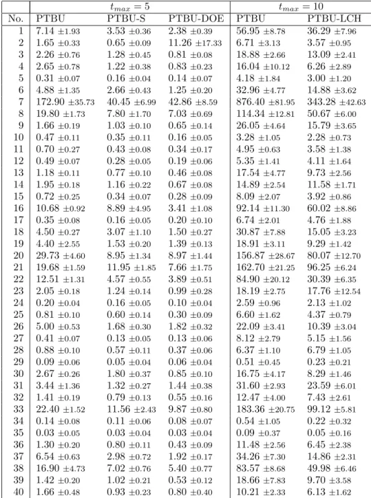
3.4 Mean accuracy measures with standard deviation comparing PTBU, PTBU-S and PTBU-DOE with τ = 0.1 and tmax = 5 on the left side. On the right side comparing PTBU and PTBU-LCH with k = 5 and tmax= 10. . . 54

3.5 Mean training runtime measures with standard deviation comparing PTBU, PTBU-S and PTBU-DOE with τ = 0.1 and tmax = 5 on the left side. On the right side comparing PTBU and PTBU-LCH with k= 5 andtmax = 10. . . 55

3.6 Average classification rates and standard deviation on test sets. . . 64

3.7 Difference in accuracy between training and test data . . . 66

3.8 Mean time and accuracy results (including standard error) of the com-parison between PTTD and PTTD-PH for differentdmax values. . . 74

3.9 Mean time and accuracy results (including standard error) of the com-parison between PTTD, PTTD-R and PTTD-fast for different training set sizes. . . 77

4.1 Wins of PTTD vs. PTTD-CI in terms of predictive accuracy and training runtime. . . 85

(16)

4.2 Predictive accuracy and training runtime results of PTTD and PTTD-CI for 40 benchmark datasets. . . 87 4.3 Average classification rates and standard deviation on test sets. . . 94 4.4 Average ranks of the algorithms (Quade) and results of the Holm test

(p-value and rejection of null hypothesis at the 5% significance level) . . 95 4.5 Experimental results in terms of RMSE. Additionally, for each dataset,

the rank of each method is shown in brackets. . . 97 5.1 An overview of some properties of the related model classes discussed in

this chapter. . . 100 7.1 Predictive accuracy results for different surrogate loss functions used

during induction withthe PTBU algorithm. Results include mean and standard deviation. . . 116 7.2 Part I: Mean accuracy measures with standard deviation comparing

PTBU-DOE with different values of τ (0.1−0.5). . . 118 7.3 Part II: Mean accuracy measures with standard deviation comparing

PTBU-DOE with different values of τ (0.6−1.0). . . 119 7.4 Part III: Mean accuracy measures with standard deviation comparing

PTBU-DOE with different values of τ (1.1−1.5). . . 120 7.5 Part IV: Mean accuracy measures with standard deviation comparing

PTBU-DOE with different values of τ (1.6−2.0). . . 121 7.6 Part I: Mean accuracy measures with standard deviation comparing

PTBU-LCH with different values ofk (1−5). . . 123 7.7 Part II: Mean accuracy measures with standard deviation comparing

PTBU-LCH with different values ofk (6−9). . . 124 7.8 Accuracy results of the three main variants selected for comparison in

Section 4.2. . . 126 7.9 Training runtime results in seconds (s) of the three main variants selected

(17)

1

Introduction

1.1

Machine Learning

Machine learning is one branch of the broad research field ofArtificial Intelligence (AI). The primary goal of machine learning is to develop strategies, i.e., computer programs, which make use of data to improve their behavior. To be a bit more formal, I want to recall a more prominent definition by Tom M. Mitchell:

“A computer program is said to learn from experience E with respect to some class of tasks T and performance measure P, if its performance at tasks in T, as measured by P, improves with experience E.” [67]

Several components are involved in this brief definition: To start with, we are talking about computer programs, the core of which mostly is an algorithm. Informally, an algorithm takes input values, processes these in a predefined sequence of instructions and returns a result as an output [26]. In general, algorithms are designed to solve well-defined problems. In the early days of computer science, several frameworks have been developed to describe the type of tasks (also called problems), which can be solved by certain kinds of algorithms. Some famous ones are: theTuring machine [103] introduced by Alan Turing and the lambda calculus [23] by Alonzo Church, just to name two.

Independent of the concrete definition, all these frameworks share one property: the algorithms have to be developed and implemented by humans. This circumstance introduces at least two difficulties: first, the programmer would need to know a solution to the problem at hand, and second, available human resources in terms of programming

(18)

craft are limited in number. These factors hinder the development of algorithms for difficult problems, because neither an exact nor an approximate solution is known or the implementation might take too long or costs too much to be economically efficient. Examples of such tasks can be drawn from many domains like biology, medicine, multi-media, finance and many more. Some examples are:

• determining the most effective medication for a given patient (medicine)

• recognizing and determining concepts like faces or other objects in digital images (multi-media)

• determining the risk of a loan default (finance)

• determining the quality of a good, produced in a factory (production)

These are just a few examples of typical tasks for which machine learning is used. The wide spectrum of industrial sectors involved already foreshadows the huge amount of potential applications of machine learning. However, there is also a potential draw-back in using a learning algorithm compared to a classical algorithm (if existing). The latter usually provides properties like completeness and correctness. In this case, a correct solution is provably existing for every instantiation of the problem at hand. In contrast, a learning algorithm usually does not guarantee a perfect solution. Rather, it produces a model which mimics the unknown mapping between a problem, taken as input, and its solution, provided as output with the help of examples provided as data. Coming back to the definition by Mitchell, a machine learning approach to the above problems uses data – referred to as experience – in order to enable the computer to learn and improve according to some predefined performance measure.

In the remainder of this thesis, we will focus on a specific but still prevalent problem of machine learning i.e. supervised learning. It is also referred to by learning from examples. In the following, we will briefly introduce the basic setting and notation. For a more comprehensive introductions see [34, 46].

Supervised Learning

Data usually comprises a set of examples. Emanating from a supervised learning [46] setting, an example is a tuple (x, y), where x= (x1, . . . , xm) ∈Xdenotes the input –

(19)

1.1 Machine Learning

also called instance – and y ∈Y denotes the output. X= X1 ×. . .×Xm denotes the

instance space, from which each instance is drawn. It often conforms to the Cartesian product of domainsXj, also referred to as attributes. Depending onY, several different

learning tasks can be distinguished. IfYis a set of categorical values, the task is about

classification. IfYequals the real numbers R, it is aregression task. Some more types

of learning problems will be introduced later.

Given atraining dataset T∈(X×Y)n, the aim of a supervised learning algorithm

Ais to find a mappingM :X→Y. Thus Aitself implements a mapping

A: [

n∈N

(X×Y)n→H.

H denotes the so-called hypothesis space. M is called hypothesis or model. Applying the model to an instance produces aprediction M(x) = ˆy.

In accordance with Mitchell’s definition, it is not enough to find an arbitrary hy-pothesisM. Instead, M must be evaluated in terms of a performance measure, which we seek to maximize. Or, equivalently, a loss functionL: (Y×Y)→Rto be minimized.

To be more precise, the ultimate goal is to find a modelM∗, which minimizes therisk of error R: M∗= argmin M∈H R (M) = argmin M∈H Z (x,y)∈(X×Y) P((x, y))·L(y, M(x)) d(x, y) (1.1)

Pdenotes the joint probability distribution overX×Y. SincePis usually unknown,

in practice, we have to rely on an estimate ofR. One common possibility is to use the

empirical risk Remp:

M∗= argmin M∈_H R emp₍_M_{) = argmin} M∈_H 1 |V| X (x,y)∈V L(y, M(x)) (1.2)

The validation set Vis a set of examples, which has not been seen by the learning algorithm before, and which we assume is drawn from the same distribution as the training dataset T. Since T and V are just samples, one seeks to be more sure about the risk estimate by repeating the steps of training and validation several times. A popular procedure in this regard iscross-validation. Given a datasetD, cross-validation randomly splitsDintok folds. Then the following steps are repeated for every fold:

(20)

1. Put the selected ith _{fold aside and run the learning algorithm on the remaining}

k−1 folds.

2. Calculate an error estimation on the ith fold.

In the end, all k error estimations are averaged. In practice, this procedure is used for model selection, i.e. many potential hypothesis classes are evaluated and the one which performs best usually is chosen for production. Since, this way the validation set become an intrinsic part of learning, the estimated error on the validation data is most often to optimistic. Therefore, it is recommended that another dataset, thetest set, is used to estimate the most realistic performance for a productive system.

Capacity Control

The kind of error we are interested in is the so-called generalization error. We are explicitly interested in a small error on unseen data. Or, the other way around, we are not primarily interested in a low training error (the error on the training set); because a low training error does not necessarily imply a small generalization error. A model with a low training error and a high generalization error is likely tooverfit the data it has seen. This is especially dangerous if a model class is very flexible like it is the case for FPTs.

In order to explain these phenomena, we assume some underlying (still unknown) data generating process, specified by P. This might for example be an underlaying functional relationship between the input and output variables. Since we are ignorant about the true relationship, we have to make some assumptions about it. This we do by selecting a hopefully well fitting model class (e.g., polynomials of degree 2). These assumptions strongly influence the learning process. Their implication on the resulting model is also calledinductive bias. Since we only make a guess about the correct model class, it is possible, that we either under- or overestimate their true complexity. For example, if the correct model class would be a polynomial of degree 3, then we have underestimated their complexity and we might encounter underfitting, whereas if the correct model class is a polynomial of degree 1 (linear function), then we are prone to overfitting.

There are many so-called regularization techniques to avoid overfitting [4, 15, 34]. Generally, they are based on the idea to restrict die complexity of a model class. The

(21)

1.2 Fuzzy Set Theory

specific technique to use of course strongly depends on the model class at hand. Stick-ing to the above example of polynomials, one way of restrictStick-ing complexity would be to upper-bound the maximum degree of the polynomials considered during learning. Furthermore, another common approach is to constraint the weight vector, making sure the weights are small in magnitude. This is referred to asshrinkage. Other model classes like decision trees [85] and also, as will be seen in later sections, fuzzy pattern trees can be regularized by restricting the size of a model. In this regard, the notion “size” will be defined as the number of subcomponents of the model and we will see, that this is a reasonable measure for its complexity.

As a side remark, the different goals of minimizing generalization vs. minimizing training error is also one of the main differences between the fields of machine learning and optimization [95].

1.2

Fuzzy Set Theory

Lotfi A. Zadeh first introduced his concept of a fuzzy set in [118]. Fuzzy sets extend the mathematical concept of a (regular or ordinary) set by allowing elements to be contained in the fuzzy set to a certain degree. To be more precise, a fuzzy set A is identified by its so-called membership function µA. A membership function is a

mapping µ : X → [0,1], where X denotes the domain or the universe of discourse. Elements x ∈X belong to A to the degree of membership (or simply degree) µA(x).

Note that µA(x) can take any value in the unit interval. As a special case, when µA

can only take two values (0 and 1), it is reduced to the characteristic function of an ordinary set.

Common choices for membership functions are piecewise linear functions like bounded linear functions, triangular or trapezoidal functions. Furthermore, also Gaussian mem-bership functions are used in many applications.

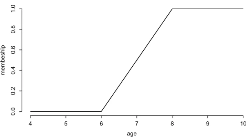
Zadeh’s intention was to enable a human user to precisely express his subjective perception of classes of objects, commonly refereed to in natural language. Examples are ”short people”, ”much older than 5 years”, or ”high temperature”. In the following, we will refer to such classes as fuzzy concepts or fuzzy terms. A membership function for the second fuzzy concept, which refers to numbers, might be the one illustrated in Figure 1.1.

(22)

age membeship 4 5 6 7 8 9 10 0.0 0.2 0.4 0.6 0.8 1.0

Figure 1.1: One possible formulization of a subjective perception of the fuzzy concept ”much older than 5 years”.

Working with fuzzy sets requires the ability to apply set operations. Basically, operations on fuzzy sets are defined in terms of their membership functions: The com-plement of A as denoted by ¯A is defined by µ_A¯ = 1−µA. Three more notions play a

central role for ordinary sets as well as for fuzzy sets. These arecontainment (A⊂B),

union (A∪B) and intersection (A∩B), which can be defined as:

• ∀x∈X : A⊂B ⇔µA(x)≤µB(x)

• ∀x∈X : µA∪B(x) = max(µA(x), µB(x))

• ∀x∈X : µA∩B(x) = min(µA(x), µB(x))

The operators (min and max) above, are the ones originally used by Zadeh. Mean-while, many more operators have been found, which can replace min and max, while keeping the same semantics of a conjunctive, respectively disjunctive, aggregation. These classes of operators are calledt-norms and t-conorms [59].

A t-norm >(·,·) is a generalized conjunction, namely a monotone, associative and commutative [0,1]2→[0,1] mapping with neutral element 1 and absorbing element 0. Likewise, a t-conorm⊥(·,·) is a generalized disjunction, namely a monotone, associative and commutative [0,1]2_→_[0_,_{1] mapping with neutral element 0 and absorbing element} 1.

(23)

1.2 Fuzzy Set Theory membership 0 1 0 1 2 3 4 5 6 "around 2" "around 4" membership 0 1 0 1 2 3 4 5 6

"around 2 and around 4"

number membership 0

1

0 1 2 3 4 5 6

"around 2 or around 4"

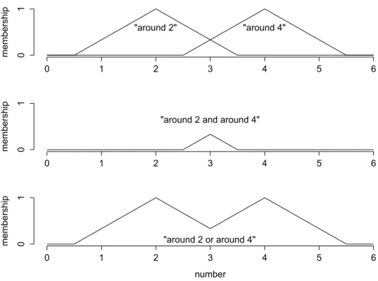
Figure 1.2: Example of two fuzzy numbers (top), which are combined with the minimum t-norm (middle) and with the maximum t-conorm (bottom).

Using t-norms and t-conorms, more complex fuzzy sets can be constructed by com-bining basic fuzzy sets. One simple example is shown in Figure 1.2. Starting with the fuzzy sets of two fuzzy numbers, namely around 2 and around 4 (top), one is able to derive the membership function of numbers, which belong to both sets simultaneously. In this example, the minimum operator was used as corresponding t-norm. The name of the derived fuzzy set might bearound 2 and around 4. In the same way, the member-ship function of numbers, which are around 2 or around 4 (bottom), is derived using the maximum operator.

Semantics of Fuzzy Sets

So far, we have set the theoretical foundations of fuzzy sets and their membership functions without caring about their semantics. Given a fuzzy setF and an elementx, what does it actually mean when we say: “µF(x) = 0.7”?

(24)

Like for probability theory, where probability is given a semantic meaning by either the “frequentist”, the “subjectivist” or even some other less prevalent views [33], for fuzzy set theory there exist at least three different meanings referring to a degree of membership. Dubois and Prade gave a comprehensive overview of possible semantics in their work [31].

• Similarity: This view relates membership degrees to distances. This view is prevalent in many data analysis applications, where the distance to prototypical elements defines the membership i.e. the proximity of other elements to a class or cluster. It is supposable the oldest view and was suggested in [10].

This view will also be the basis for this work and the methods which will be introduces in the following chapters.

• Utility: F in this case embodies a set of more or less preferred elements; µF(x)

then determines theutilityof each element. That is,µF(x) refers to the usefulness

of x. This way fuzzy sets can act as soft constraints to optimization problems. The view was put forward in [11].

• Uncertainty: Zadeh introduced this interpretation in his works about possibility theory[120] andapproximate reasoning [119]. A membership valueµF(x) in these

frameworks means the degree of possibility that a parameterx has a valueu.

Towards Classification

Being able to dynamically construct more complex fuzzy sets with the help of fuzzy logical operators is especially interesting from a machine learning perspective. Fuzzy sets can be used asgradual / fuzzy selectors of instances, which e.g. shall belong to the black class in Figure 1.3. There, a simple two-dimensional example is presented.

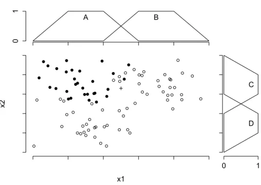
The instances are represented by a vector (x1, x2). As can be seen in the figure, they are obviously arranged in three major groups, which are to some extent overlapping and may not be clearly separated from each other easily. Two of the groups belong to the white class (bottom-left and up-right), the other one belongs to the black class (top-left). At the top and the right axis of the scatter plot, trapezoidal fuzzy sets are shown (A, B and C, D), which are defined on their respective domain. Of course,

(25)

1.2 Fuzzy Set Theory x1 x2 A B 0 1 C D 0 1

Figure 1.3: Example of elements existing in a 2-dimensional space, i.e. described by two attributes (x1, x2).

this example is idealized; in reality, class distributions seldom appear in such a strict arrangement.

Considering the task to select the instances of the black class, a reasonable choice of a fuzzy selector would be:

µSblack(x1, x2) =>(µA(x1), µC(x2)). (1.3)

Sblack as defined by its membership function in (1.3) conjunctively combines the

two fuzzy setsA and C. Roughly speaking, in order to belong to the fuzzy setSblack,

an instance has to belong to both fuzzy setsA and C, simultaneously. Here, the term ”belonging to” refers to a high membership value, i.e., the instance has to produce a high output for both membership functions.

In the same way, we are able to create a fuzzy set for the white class:

(26)

First we select each of the two white groups individually as we did before for Sblack,

and then we aggregate them using a t-conorm. In words: An instance belongs to the white class, if it either belongs toB and C or it belongs toAand D.

Membership in this case is interpreted as similarity. Taking fuzzy set Sblack as an

example, it is constructed in a way, that it relates the membership of an element to its proximity to elements of the black class. The same applies forSwhite, respectively.

This example already reveals an important benefit of using a fuzzy set instead of using an ordinary set in order to select instances of one class. The boundaries of the two classes are blurred, which is a common phenomenon in machine learning. Assuming sharp class boundaries when using ordinary sets (i.e. intervals) would not properly reflect the reality of the class distributions. Instead, for an instance, for which we do not know the actual class label and which is close to the class boundaries, both classes appear to be valid options to some degree.

Let us look at the instance xcross like the one indicated as a cross in Figure 1.3.

Concerning the white class, xcross is located at the margin of the group of white

ele-ments, still within reach but also not directly covered. Hence, it seems reasonable to not give a full membership of 1 nor a membership of 0. The same reasoning also applies to the black class, independently.

After constructing Sblack andSwhite we not only have a fuzzy logical description of

the two classes but we are also able to predict the class of an unknown instance x0. To this end, we simply compare the membership values Sblack(x0) and Swhite(x0) and

decide for the class with the higher membership.

As we already started to introduce fuzzy set theory in the realm of machine learning, in the following section we will further focus on this symbiosis.

1.3

Fuzzy Sets in Machine Learning

In the past, fuzzy set theory has already been used in the realm of machine learning in several regards. These include applications like fuzzy clustering [48], fuzzy rule-based systems [99, 109],fuzzy decision trees [54, 110] and fuzzy association analysis [21, 29], just to name a few.

In [51], H¨ullermeier points out some potential contributions of fuzzy set theory to the field of machine learning. These include the ability to express fuzzy (or gradual)

(27)

1.3 Fuzzy Sets in Machine Learning

concepts, like the ones we have discussed in the last section. In traditional machine learning, acquiring a definition of a general (non-fuzzy) concept by a set of positive and negative examples is also called concept learning [6]. Formally, a concept usually is expressed in terms of predicates, which are conditions on the properties of the ob-jects. For example, a bird is asmall to medium size, winged, feathered, usually able to fly animal. Extending concept learning to the fuzzy case has the following potential advantages:

• Many real world concepts are fuzzy by nature and do not have sharp boundaries. Therefore, it is inappropriate to make use of sharp constraints where there is no sharp boundary in the real world. Allowing fuzzy predicates enriches the concept description and makes it more realistic.

• A fuzzy concept can be considered particularly robust in the following sense: Comparing a standard interval on the real numbers with a fuzzy interval (trape-zoidal fuzzy set), the former is prone to a strange ”boundary effect”, whereas the latter is not. This effect refers to the fact that a small variation of the boundary points of the interval may have a strong influence on the model in the interval case. The effect is alleviated when using fuzzy sets instead of intervals.

• Fuzzy set theory provides an interface between an arbitrary (most often a nu-meric) scale and a symbolic scale, which usually consists of linguistic terms. This provides a first layer of abstraction by utilizing natural language to describe complex objects. This potentially improves the interpretability of the formal description of a concept.

• In line with their improved interpretability, many fuzzy methods enable us to combine modeling and learning. This is especially true for rule-based systems as well as fuzzy pattern trees. For rule-based systems, experts are able to formulate if-then rules, roughly describing the input-output relation of the system. Then, implementing the linguistic terms employed by the expert in terms of fuzzy sets, we are able to tune the parameters of these fuzzy sets in an optimal way using the data we have observed. This is just one example of incorporating expert knowledge into the learning process. Many more variants can be thought of.

(28)

(29)

2

Fuzzy Pattern Trees

Fuzzy Pattern Trees (FPT) have independently been introduced by Huang et al. [49] and Yi et al. [116], who called this type of modelFuzzy Operator Trees. The FPT model class is related to several other model classes includingfuzzy rule-based systems (FRBS),

fuzzy decision trees (FDT) and genetic programming (GP). These model classes and their respective differences in comparison to FPTs are discussed in Chapter 5.

In this chapter we first introduce the basic constituent parts of the model class, then these parts are assembled into a fuzzy pattern tree. The introduction is followed by a discussion about the interpretatability of FPTs and the potential capability of an expert to use the model class for typical modeling [71, 72, 91] and machine learning tasks. After this, we focus on some aspects of FPTs, which are adjuvant in many applications and also form the first contributions of this thesis.

2.1

Model Overview

A fuzzy pattern tree is a hierarchical, tree-like structure, whose inner nodes are marked with generalized (fuzzy) logical and arithmetic operators, and whose leaf nodes are associated with fuzzy predicates on input attributes. It propagates information from the bottom to the top: A node takes the values of its descendants as input, aggregates them using the respective operator, and submits the result to its predecessor. Thus, an FPT implements a recursive mapping producing outputs in the unit interval.

(30)

high quality wine AVG (Criterion I) OR alcohol is high density is high (Criterion II) OR (Criterion III) AND alcohol is low acidity is low sulfates is high

Figure 2.1: An interpreted example of a fuzzy pattern tree.

dataset1. It represents the fuzzy concept – a fuzzy criterion for – wine with a high quality. The node labels of the tree illustrate their interpretation and not yet their implementation.

In order to interpret the whole tree and grasp thefuzzy pattern it depicts, we start at the root node. It represents the final aggregation (a simple average in this case) and outputs the overall evaluation of the tree for a given instance (a wine). Then, we proceed to its children and so forth. The interpretation could be like this:

A high quality wine fulfills two criteria, which are able to compensate each other. We call these two criteria – the left and right subtree of the root node – criterion I and criterion II. Criterion I is fulfilled if the alcohol concentration of the wine is high or its density is high. Criterion II is fulfilled, if the wine has a high concentration of sulfates or a third criterion (III) is met. This is the case, if both alcohol concentration and the wines acidity is low.

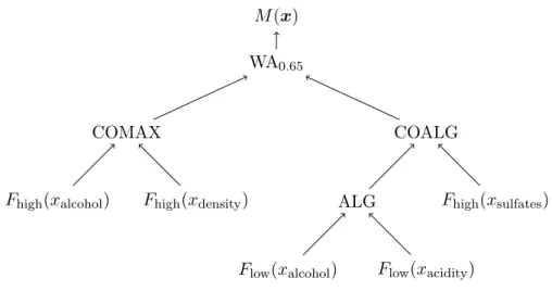
Next, we will proceed with the implementation of the tree. Figure 3.17 shows the same model, but this time with more detailed information about the concrete operators, their parameters and the fuzzy sets involved. The average in the root node is realized by a weighted average operator (WA), which assigns the weight 0.65 to the left subcriterion, whereas the right one receives the remaining weight of 0.35. The AND and OR nodes are implemented by generalized logical operators (t-norms and t-conorms). Finally,

(31)

2.2 Aggregation and Structure

M(x) WA0.65

COMAX

Fhigh(xalcohol) Fhigh(xdensity)

COALG

ALG

Flow(xalcohol) Flow(xacidity)

Fhigh(xsulfates)

Figure 2.2: The same FPT as in the previous figure with additional information about the implementation of each node.

fuzzy sets – defined on their corresponding attribute domains – will be used in order to express the fuzzy linguistic terms contained in the leaf nodes.

2.2

Aggregation and Structure

As described above, internal nodes represent the aggregation of two membership val-ues. The original set of aggregation operators used in [49] include three families of aggregation operators. These are generalized conjunctions (t-norms) and generalized disjunctions (t-conorms) as they where introduced in Section 1.2. Furthermore, two different averaging operators are used, which are the simple weighted average and the

ordered weighted average [90, 114].

The operator set used in [49] is shown in Tables 2.1–2.2. The variables u and v denote the membership values, to be aggregated.

An ordered weighted average (OWA) combination of k numbers v1, v2, . . . , vk is

defined by OWAw(v1, v2, . . . , vk) df = k X i=1 wivτ(i), (2.1)

whereτ is a permutation of{1,2, . . . , k}such that v_τ₍₁₎≤v_τ₍₂₎≤. . .≤v_τ₍_k₎ and w= (w1, w2, . . . , wk) is a weight vector satisfyingwi ≥0 fori= 1,2, . . . , kandPki=1wi= 1.

(32)

Name Definition Code

Minimum min(u, v) MIN

Algebraic uv ALG

Lukasiewicz max(u+v−1,0) LUK Einstein ₂₋₍_u₊uv_v₋_uv₎ EIN

Table 2.1: Fuzzy operators: t-norms

Name Definition Code

Maximum max(u, v) MAX

Algebraic u+v−uv COALG

Lukasiewicz min(u+v,1) COLUK

Einstein ₁₊u+_uvv COEIN

Table 2.2: Fuzzy operators: t-conorms

by a set of weights. However, a weight does not directly refer to an argument, like in WA, but instead to a rank: wi is the weight of the i-th smallest value among

v1, v2, . . . , vk.

Note that fork= 2, which is the case of FPT, (2.1) boils down to

OWAγ(u, v) =γ·min(u, v) + (1−γ)·max(u, v), (2.2)

which is simply a convex combination of the minimum and the maximum. In fact, the minimum and the maximum operator are obtained, respectively, as the two extreme casesγ = 1 and γ = 0.

When defining an order relation ”” on aggregation functions in agreement with the standard (point-wise) order on functions, then conjunctive aggregationsAare those withAmin, compensatory (averaging) those withminAmax, and disjunctive those for which maxA [41].

Therefore, the class of OWA operators nicely “fills the gap” between the largest conjunctive combination, namely the minimum t-norm, and the smallest disjunctive combination, namely the maximum t-conorm.

(33)

2.2 Aggregation and Structure

2.2.1 Extending the Set of Operators

The original selection of operators is to some extent arbitrary. In general, there exist many different t-norm and t-conorms. Especially, there are parameterized families like theDubois & Prade t-norm [35],

DPα(u, v) =

u+v−uv−min(u, v,1−α)

max(1−u,1−v, α) , where 0≤α≤1 (2.3)

theHamacher t-norm [45] Hα(u, v) =

uv

α+ (1−α)(u+v−uv), where 0≤α≤+∞ (2.4) and many more. Parametric operators like these have an important advantage in the realm of machine learning. Their parameters can be optimized to best fit the data at hand. This potentially allows a more accurate fit of the overall model. It should be noted, however, that allowing for more and more operators also yields a higher runtime of the learning algorithms, which will be introduced in Chapter 3. Therefore, it is desirable to find a set of operators, which on the one hand is small and can efficiently be optimized, and on the other hand is at least as expressive as the original operator set. So far, we are not aware of a single parameterized operator family, which could be used to substitute all originally used t-norms, respectively t-conorms. In the following, three parameterized operators are proposed to be used for the FPT model class, one for each class of aggregation operators: t-norms, t-conorms and averaging operators.

To start with, WA and OWA are replaced by the so-called Choquet integral (CI) [41]. In order to define this operator in a formally correct way, it should be written as an integral of a function with respect to a suitable non-additive measure. However, in the discrete case with only two input arguments, one can show that it reduces to the following simple expression:

CI(u, v) = (

(1−β)u+βv ifu≤v

αu+ (1−α)v ifu > v , (2.5)

where α, β ∈ [0,1]. Note the following special cases: CI = min and CI = max for (α, β) = (0,0) and (α, β) = (1,1), respectively; forβ= 1−α, one obtains the WA and forβ=α the OWA operator.

(34)

Especially interesting from a computational point of view, is the existence of an efficient way to approximate the optimal parameters α and β. For this purpose, we first use a closed form solution in order to minimize the squared loss of the operator on our training data. This solution, however, does not ensure the parameters to reside in [0,1]. Hence, we simply force them to: If α is smaller than 0, we set it to 0; if it is bigger than 1, we set it to 1. The same procedure is applied to β. This may yield a suboptimal solution, however, in the general case it is assumed to be close to optimal. This procedure is commonly used for constraint optimization problems [18] and was also implemented by Huang et al. to determine the parameters of the WA and OWA operators.

In order to further provide a real extension of the current t-norms, respectively t-conorms, we use two convex combinations:

CC(u, v) :=γ1·MIN(u, v) +γ2·ALG(u, v)+ γ3·LUK(u, v) +γ4·EIN(u, v)

COCC(u, v) :=γ1·MAX(u, v) +γ2·COALG(u, v)+ γ3·COLUK(u, v) +γ4·COEIN(u, v) where γi ≥0, i∈ {1,2,3,4} and 4 X 1 γi = 1.

Note that CC and COCC are actually no longer t-norms, respectively t-conorms, be-cause they do not satisfy the associativity property. However, one can easily prove, that CC is aweak t-norm and COCC is aweak t-conormas they were introduced by Yager in [115]. Although CC and COCC do not satisfy associativity, they at least satisfy quasi-associativity. Furthermore, associativity is never used in the realm of FPT. Although the interpretation of weak t-(co)norms is not exactly the same as of t-(co)norms, [115] describes them as being “and-like” and “or-like”, respectively. This is obvious for some special cases ofγi. Whenever there is one γi, which takes all the weight (e.g. γ1 = 1), the CC and COCC operators actually coincide with the i-th t-(co)norm.

In order to find good parameters for these operators as well as parametric t-norms and t-conorms, there might be the need for optimization methods likegradient descend

(35)

2.3 Important Properties of Fuzzy Pattern Trees

2.3

Important Properties of Fuzzy Pattern Trees

Apart from the properties of the FPT model class we already discussed, it exhibits two other very interesting properties.

Monotonicity

The first one is the ability to modelmonotonicity constraints[32, 79]. The type of mono-tonicity constraint which is meant here refers to the type of mapping a tree implements. All operators introduced so far are monotonically increasing in their arguments, i.e.

µA(x)≤µA(x0) and µB(x)≤µB(x0)⇒φ(µA(x), µB(x))≤φ(µA(x0), µB(x0)), (2.6)

whereφ(·,·) denotes an operator, µA(·) andµB(·) denote membership functions andx

andx0 denote attribute values. Since every single operator is monotonically increasing, every composition of these operators is also monotonically increasing. This means that the whole tree is monotonically increasing in the membership values given by the leaf nodes. Therefore, the question of how the output of the tree is influenced by an attribute depends on how the leaf nodes’ membership depends on its attribute.

Note however, that the fuzzy sets in a tree are not necessarily monotonic. A regular triangular or trapezoidal fuzzy set, for example, is not a monotonic function. Never-theless, there are of course fuzzy sets, that are monotonic (e.g. Figure 1.1). They can even be monotonically increasing or decreasing. This actually allows us to constrain the influence of each single attribute in a way, which is suggested by background knowledge about the problem domain.

Consider, for example, the problem of making a diagnosis for a given patient. To be able to decide whether or not the patient is suffering from a certain disease, the physician conducts several tests – e.g. measuring the temperature, blood pressure, gathering important information by asking the patient or even measuring the level of certain ingredients in the blood of the patient. Assuming that each single test returns a score (or probability), in many cases these scores monotonically increase or decrease together with the risk of actually suffering from the disease. TheMarburg heart score

[19] constitutes a prevailing example. Roughly speaking, it aggregates several risk factors for the purpose of predicting a severe heart disease. The presence compared to

(36)

the absence of a risk factor, in this case, shall only increase the probability of suffering from the disease.

In order to learn an aggregation function on data of that kind, monotonically con-straining the influence of each single test by only allowing monotonically increasing fuzzy sets like ’high of age’ (cf. Figure 1.1) can guide the learning process and improve the results.

This is especially true for problems with sparse data as was shown in [5]. Sparsity in this regard means that there are only relatively few observations available to learn from, compared to the dimensionality of the problem. This situation is also referred to as curse of dimensionality [9]. Roughly speaking, when the dimensionality increases, the volume of the instance space and in the same way the size of the hypothesis space increases so fast that the available data becomes sparse. In this case, each type of background knowledge reducing the model space, including monotonicity constraints, will be useful.

Handling Missing Values

A common obstacle in machine learning is the problem of dealing withmissing values. A missing value refers to the absence of a value for a certain attribute of an instance. Missing values can be treated in many different ways, depending on the assumptions about the reason of missing the value. In the literature [87, 89], three main types are distinguished, namely missing completely at random (MCAR), missing at random

(MAR) andmissing not at random (MNAR).

MCAR denotes the situation where missing values of an attribute occur for a random subset of instances. The second type denotes missing values, which occur (statistically) depending on an observed attribute. In this regard, the name MAR is vexing, since the values do not occur completely at random considering the information of the de-pendent attribute. Nevertheless, the dependence between an observed attribute and the occurrence of a missing value in another attribute may be of any strength. Except for full dependence, the occurrence stays random. MNAR denotes the setting, when the reason for a missing value (potentially fully) depends on unknown or unobserved information.

It can be determined from data, whether data is MCAR, whereas it is impossible to determine the cases of MAR and MNAR [87, 89].

(37)

2.3 Important Properties of Fuzzy Pattern Trees

The simplest way to handle missing values is to entirely exclude instances with missing values from the dataset, which is called complete case analysis. When data is MCAR, complete case analysis leads to unbiased results. However, in many cases data is not MCAR, but MAR or MNAR. In these cases, omitting every incomplete instance leads to biased results [89]. Another drawback of the complete case analysis is a loss of information. Especially for small datasets with many missing values, this reduces the information to learn from dramatically. Therefore, it is desirable to deal with incomplete instances differently.

Depending on the machine learning technique one wants to apply, it is necessary to include a preprocessing step and applyimputation methods. These methods replace missing by estimated values. How the estimations are calculated depends on the impu-tation method. Van Buuren provides an overview on impuimpu-tation techniques in [104]. However, it is more elegant, if a machine learning method is capable of directly dealing with missing values in a reasonable way. For FPT, this is the case, as will be explained in more detail in the remainder of this subsection. To this end, we will show how a tree is evaluated in case of missing values. This is sufficient for all of our current induction algorithms to work properly with missing values.

Assuming that we have to determine the membership degree of an instance x˜ ∈X

with missing values for the fuzzy pattern treeM, we will make use of the monotonicity of the tree in the following way. x˜ shall exhibit missing values at an arbitrary but positive number of attributes, for example x˜ = (x1, x2,ø, x4,ø), where ø denotes a missing value. In this example, the values for the third and fifth attribute are missing. For simplicity and without loss of generality, we also assume that there is only one fuzzy set for each attribute (µ1(·), ..., µ5(·)). This means, that we are not able to evaluate the fuzzy sets µ3(·) and µ5(·), but we definitely know in which range the unidentified membership values must reside, namely [0,1].

Now, for the following, it is adjuvant to defineM to beM after replacing all fuzzy sets in the leaf nodes by the identity functionid(·). Then it yields that

M((·,·,·,·,·))≡M((µ1(·), µ2(·), µ3(·), µ4(·), µ5(·))). (2.7) Due to monotonicity, we additionally know that

(38)

ν:= M((µ1(x1), µ2(x2),0, µ4(x4),0))

≤ M((µ1(x1), µ2(x2),1, µ4(x4),0))

≤ M((µ1(x1), µ2(x2),1, µ4(x4),1)) =:ν

Due to the monotonicity of the tree in the membership values, we can now conclude, that the proper membership degree for the incomplete instance x˜ must reside in ν = [ν, ν]. In principle, this interval could be directly returned to the user. Although, we were not able to identify the proper exact membership because of the missing information, at least we are able to confine the interval of possible values. If we are forced to make a point prediction, the simplest way is just predicting the mean ofν, ν. Depending on the learning task, which we will discuss in the next chapter, it is sometimes already enough to know ν in order to make a prediction (e.g., in classifica-tion). Additionally, we will see that we can utilize the ability to determineν efficiently, in order to reduce the costs of a prediction.

2.4

Universal Approximation Property

As we have seen in the Chapter 1, learning in our case involves the minimization of the empirical risk (1.2). Assuming our data comes from a probabilistic data generating processPand let

f(x) = argmin ˆ y E(L(ˆy, y)|x) (2.8) = argmin ˆ y Z L(ˆy, y) dP(x, y) (2.9)

be the so-called Bayes predictor, which attains the lowest possible prediction error. Then the question arises, if we are able to closely approximate f by means of a fuzzy pattern tree model. This would be a hint towards the belief that we are able to succeed in the minimization of (1.2).

(39)

2.4 Universal Approximation Property

To be more precise, in this section, we will give a proof, that there always exists an FPT M to approximate an arbitrary function g : [0,1]m → _R up to any degree of accuracy. This ability is called universal approximation property.

The proof is constructive in the sense that given a functiong, we construct an FPT, which implements a function ˜g, to fulfill the desired approximation.

Theorem. (FPTs are Universal Approximators) Let m ∈ _N and g : [0,1]m → [0,1]

be an arbitrary continuous function. Let ∈_R with >0. Then, there exists a fuzzy pattern tree M, which implements a function g˜, with

|g(x)−g˜(x)|< ∀x∈[0,1]m.

Proof. Because g is continuous, for every x1 ∈ [0,1]m and every > 0 there exists a δx1,>0, such that

∀x2 ∈[0,1]m:|x1−x2|< δx1,⇒ |g(x1)−g(x2)|< (2.10)

(Weierstrass definition) [86]. Because a continuous function, defined on a compact set isuniformly continuous, it even holds that:

∃δ>0 ∀x1,x2∈[0,1]m:|x1−x2|< δ ⇒ |g(x1)−g(x2)|< (2.11)

Let us selectδ according to (2.11).

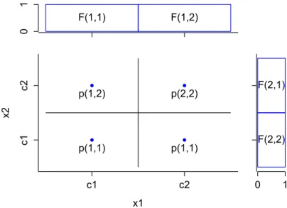
In the following, we want to span a grid in [0,1]m_{, for which it holds, that:}

∀x∈[0,1]m ∃p(j)∈G:|x−p(j)|< δ

Such a finite grid exists, because [0,1]m is bounded and δ >0. In order to create the

grid, let

γ= r

(2δ)2

m . (2.12)

γ is the maximum Euclidean distance, which two neighboring grid points may have when they get projected onto one dimension. Now, let

k= 1 γ and γ0 = 1 k ≤γ (2.13) Let{c1, c2, ..., ck}={γ 0 2, 3γ0 2 , ..., (2k−1)γ0

2 }be the possible grid point values on each single dimension. Then we finally can define the grid points as:

(40)

x1 x2 c1 c2 c1 c2 p(1,1) p(1,2) p(1,1) p(2,2) F(1,1) F(1,2) 0 1 F(2,1) F(2,2) 0 1

Figure 2.3: Example of a grid in two dimensions with two fuzzy sets for each dimension.

This yields|G|=km. Figure 2.3 illustrates the grid by an example.

For each pointp∈Glet us create a small subtreeSp, which by itself consists of two

parts: the selector subtree S_pSel and the value subtree S_pV al. Both are then aggregated by means of the conjunctive min operator. SSel

p ”selects” exactly one grid cell, which

means, it assigns full membership to those instances xthat are close enough to pand zero membership to all other. This is accomplished with the help of a set of k fuzzy setsF i, j for each of them dimensions. Thei-th fuzzy set of the j-th dimensionFi,j is

defined as: Fi,j(x) =    1 cj−γ 0 2 ≤xi < cj+ γ0 2 0 otherwise (2.15)

Figure 2.4 shows a selector for the grid cell centered by (c1, ..., c1) = (γ

0

2, ...,

γ0

2). S_pV al will output a constant value of g(p). We could either just use a constant membership function at the membership degree g(p), but this fuzzy set would not be normalized, which is a common requirement. Therefore, instead we use an aggregation of the two fuzzy sets:

low(x) =    1 x1 <0.5 0 else

(41)

2.4 Universal Approximation Property M IN . .. M IN F1,1 F2,1 F·,1 Fm,1

Figure 2.4: The implementation of the selector subtree SSel

p for the grid point p =

(c1, ..., c1).

OWA_g₍_p₎

high low

Figure 2.5: The implementation of a constant functiong(p).

high(x) =    1 x1≥0.5 0 else

Aggregating these two fuzzy sets with an OWA operator with a weight ofα=g(p) produces the desired membership function. Figure 2.5 illustrates the value subtree.

Then, we construct a tree, which implements the following function: ˜

g(x) = max

p∈G{µSp(x)}

This is achieved by successive pairwise aggregation of all subtreesSp for allp∈G.

Figure 2.6 demonstrates the tree structure.

. .. M AX M AX S_p(1) S_p(2) S_p(3) S_p(4)

(42)

Now, we have to reason about |g(x)−˜g(x)|. Letxˆ∈[0,1]m _{be arbitrary but fixed.}

LetG0 ={p∈G:|xˆ−p| ≥δ} and letG+={p∈G:|xˆ−p|< δ}. Then, it holds:

1. ∀p∈G0:µSp(xˆ) = 0

2. ∀p∈G+:|µSp(xˆ)−g(xˆ)|< 3. G+ is not empty.

Therefore, we can conclude, that also |˜g(xˆ)−g(xˆ)|< .

This proof holds for all functions g : [0,1]m → _R. In Section 3.1, however, we will introduce a technique that enables us to easily extend the input space ofg from [0,1]m to any compact set X.

2.5

Vapnik-Chervonenkis Dimension

The well-known Vapnik-Chervonenkis (VC) dimension [17, 105, 106, 107] is a general measure of the potential capacity of model classes. This number is interesting for at least two reasons. First, it provides a rough idea of how powerful a model class is. ”Powerful”, in this regard, means the ability of dealing with complex (especially non-linear) problems. Second however, for a potentially very complex model class, it is easier to overfit (see Section 1.1) than for less complex classes. This has to be taken into account when using it and therefore, we will analyze the model class of fuzzy pattern trees in the following.

Assuming a number ofdpointsX={xi|i= 1, ..., d} in the input space. Then, it is

theoretically possible to assign a positive or negative class (setting of binary classifica-tion) to every point in 2d many ways. This is equivalent to selecting a subset C ⊂X

of arbitrary size. Such a subset is also denoted asconcept.

A model class Mis said toshatter dpoints, if for every conceptC⊂Xthere exists a modelM ∈M, which isconsistent withC. Consistency, in this regard, means

M(x) = 1⇔x∈C.

The model classM exhibits a VC-dimension of d, if dis the largest number for which the above condition holds.

(43)

2.5 Vapnik-Chervonenkis Dimension

In order to prove, that the VC-dimension of a model class isd, one has to proceed in the following way. First prove that the VC-dimension is at least d and then, that it is notd+ 1. In our case however, we will easily prove that the model class of fuzzy pattern tree classifiers has an unlimited VC-dimension.

Theorem. The model class of fuzzy pattern tree classifiers has a VC-dimension of∞. Proof. Let d∈_Nbe arbitrary but fixed. Let X be a set of dpoints{x(1)_{, . . . ,}_x(d)_{} ⊂} [0,1]m. Let the elements of X+ ⊂ X be labeled positive (1) and the elements of

X−=X\X+ be labeled negative (0).

Like in the previous proof, we span a grid in [0,1]m. This time, each cell of the grid shall contain at most one pointx∈X. Such a grid exists, becauseXis finite. In order to create the grid, let

γ= min|x(_ij)−x(_ij0)|

∀i∈ {1, ..., m} and j, j0 ∈ {1, ..., d} .

γ is the minimum gab between a pair of points projected onto one dimension. Still, we need to take the smallest distance between a point and the boarders ofXinto account.

Therefore, let

γ0 = min

γ,(1−x(_ij)), x(_ij) ∀i∈ {1, ..., m} and j ∈ {1, ..., d} .

Just like before, let {c1, c2, ..., ck} = {γ

0

2, 3γ0

2 , ...,

(2k−1)γ0

2 } be the possible grid point values on each single dimension. Then we can define the grid points as:

G={(ci1, ..., cik)|cij ∈ {c1, ..., ck}} (2.16)

See Figure 2.3 for an illustration of the grid.

The construction of the tree complies with the one in our previous proof with one exception. The value subtreeS_pV al will output a constant value of 1 only in case there exists a pointxi ∈X+ located within the cell centered by p, else it outputs 0.

Concluding the construction, the resulting tree will output 1 for a pointx∈[0,1]m if and only ifxbelongs to a cell of the grid, which already contains an element ofX+_. Therefore, the output of the elements ofX+ themselves is 1. Due to the construction of the grid (each cell at most contains one element ofX) all elements ofX− receive an output of 0.

Hence, the tree shatters X and because dwas set arbitrarily we have proven that the VC-dimension of fuzzy pattern tree classifiers is∞.

(44)

This result suggests, that for arbitrarily complex concepts, there is an FPT model, which is adequate in terms of capacity. Having said that, as already mentioned before, highly flexible model classes are prone to overfitting. This is especially true, when the VC-dimension is even infinite. Theoretical results in the realm of the PAC Learning Theory [57] have shown, that it might be even impossible at all to learn for such model classes. Therefore, it is important to be able to adjust the models’ class complexity as needed.

One way of doing this is to limit the size of the trees. Smaller trees are less ex-pressive and hence exhibit a lower VC-dimension. In later sections when we introduce algorithms, for building fuzzy pattern tree models from data, we will see, that these algorithms always start with small trees, which stepwise become larger until they ter-minate. This way, the effective VC-dimension stays finite and in fact, it dynamically increases to hopefully match the complexity of the learning task.

This approach is in line with other algorithms inducing models of different model classes likerule-based systemsanddecision trees. These will be discussed in Chapter 5. Just like for fuzzy pattern trees these algorithms start with small, hence simple, models that grow until some termination criterion is met.

In the realm of PAC learning, this basic strategy is justified by theoretical results [57]. The so-called Occam algorithms not only try to find a consistent hypothesis but additionally prefer small ones. The size of an hypothesis usually is defined by the length of its representation. The idea of Occam algorithms is that a simpler hypothesis better generalizes to unseen data than complexer ones. This is basically whatOccams razor [16] suggests. Hence the name.

(45)

3

Learning Fuzzy Pattern Trees

In the last chapter, we have seen how an expert is able to model an FPT using his/her expert knowledge, hence this approach can be entitled knowledge-driven. In this sec-tion, we focus on another way of FPT construcsec-tion, namely algorithmic ordata-driven

approaches to induce FPT models. As already seen in the introductory section, data usually comprises a set of training examples

T = {(x(i), y(i))}n

i=1 ⊂X×Y .

Being able to induce FPT models utilizing data is helpful in at least two regards. First, sometimes one is facing a new prediction problem for which there is no expert knowledge available. In this situation, there is no expert able to model an FPT. And second, even though there might be expert knowledge available, comparing an expert model with an algorithmically induced model can yield new insights and ignite an alternating development process.

To this end, we will introduce several algorithms starting with an already existing one by Huang, Gedeon & Nikravesh [49], followed by several new ones. For each algorithm, we first motivate its development by a discussion about drawbacks of existing approaches, then introduce the method itself as a potential solution to these drawbacks and in the end validate its success in an experimental study.

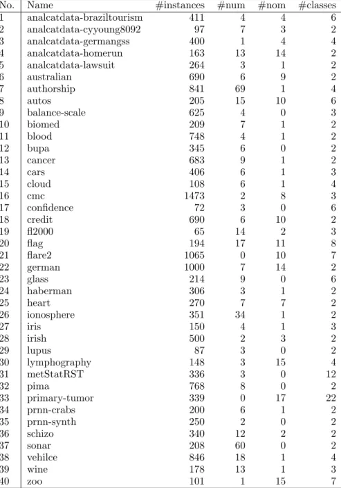
In order to provide comprehensive overall studies, the experimental setup is con-sistent throughout this work. When comparing learning algorithms1 we always use a 3-times 10-fold cross validation procedure. Most of the time we will use 40 classification

(46)

datasets listed in Table 3.1 for comparing different variants of FPT induction. How-ever, in Section 4.4 we will evaluate the performance of FPT on 12 regression datasets. Both sets are assembled from and freely available at the UCI [7] and STATLIB [66] repositories. Tables 3.1 and 3.2 also summarize some of their properties: the number of instances (#instances), the number of numerical attributes (#num) and the number of nominal attributes (#nom). Additionally, for classification datasets the number of classes (#classes) and for regression datasets the mean and the standard derivation of the output variable are provided.

Before we actually concentrate on the learning algorithms we have to take care of two prerequisites. In the following section we start with the preparation of data. Since FPTs are designed to work with “fuzzy data” and most data is not of this type, we have to add a pre-processing and a post-processing step. These steps can be implemented with the help of an expert. However, because an expert might not be available, in the following section we propose a generic way to transform regular data into data applicable to FPTs. The second requirement concerns the optimization of parameters for the newly introduced CI operator. The optimization procedure will be an important component used by every algorithm discussed.

(47)

No. Name #instances #num #nom #classes 1 analcatdata-braziltourism 411 4 4 6 2 analcatdata-cyyoung8092 97 7 3 2 3 analcatdata-germangss 400 1 4 4 4 analcatdata-homerun 163 13 14 2 5 analcatdata-lawsuit 264 3 1 2 6 australian 690 6 9 2 7 authorship 841 69 1 4 8 autos 205 15 10 6 9 balance-scale 625 4 0 3 10 biomed 209 7 1 2 11 blood 748 4 1 2 12 bupa 345 6 0 2 13 cancer 683 9 1 2 14 cars 406 6 1 3 15 cloud 108 6 1 4 16 cmc 1473 2 8 3 17 confidence 72 3 0 6 18 credit 690 6 10 2 19 fl2000 65 14 2 3 20 flag 194 17 11 8 21 flare2 1065 0 10 7 22 german 1000 7 14 2 23 glass 214 9 0 6 24 haberman 306 3 1 2 25 heart 270 7 7 2 26 ionosphere 351 34 1 2 27 iris 150 4 1 3 28 irish 500 2 3 2 29 lupus 87 3 0 2 30 lymphography 148 3 15 4 31 metStatRST 336 3 0 12 32 pima 768 8 0 2 33 primary-tumor 339 0 17 22 34 prnn-crabs 200 6 1 2 35 prnn-synth 250 2 0 2 36 schizo 340 12 2 2 37 sonar 208 60 0 2 38 vehilce 846 18 1 4 39 wine 178 13 1 3 40 zoo 101 1 15 7

(48)

No. Name #instances #num #nom mean stddev 44 auto-mpg 390 8 0 23.42 7.81 45 concrete 1030 9 0 35.82 16.71 46 flare1M 323 8 3 0.14 0.48 47 flare2C 1066 8 3 0.3 0.84 48 forestfires 517 11 2 12.85 63.66 49 housing 506 14 0 22.53 9.2 50 imports-85 205 16 10 13207.13 7868.77 51 machine 209 7 2 105.62 160.83 52 servo 167 3 2 1.39 1.56 53 slump 103 11 0 36.04 7.84 54 winequality-red 1599 12 0 8.32 1.74 55 winequality-white 4898 12 0 5.88 0.89

(49)

3.1 Fuzzification and Defuzzification

3.1

Fuzzification and Defuzzification

Fuzzification

We proceed from the common setting of supervised learning as already introduced in Section 1.1 and assume data to be a set of instances exhibiting an attribute-value representation, which means that an instance is a vector

x∈_X=X1×X2×. . .×Xm ,

whereXi is the domain of thei-th attribute Ai. In addition to these input attributes,

every instancex is assigned to an output value y∈Y. For now, we only consider two

cases: eitherY=R(regression) orY={0,1}(binary classification), where 0 indicates

the negative and 1 indicates the positive class.

Each domain Xi is discretized by means of a fuzzy partition, that is, a set of fuzzy

subsets

Fi,j : Xi→[0,1] (j= 1, . . . , ni) (3.1)

such thatPnj

j=1Fi,j(x)>0 for allx∈Xi. TheFi,j are often associated with linguistic labels such as “small” or “large”, in which case they are also referred to asfuzzy terms

(the identifier of an underlaying fuzzy concept).

To make fuzzy pattern trees amenable to numerical, ordinal, nominal or binary attributes, these attributes have to be “fuzzified” and discretized beforehand. The fuzzy partitions are either provided by an expert, who uses his expert knowledge to define comprehensible and reasonable fuzzy sets for each attribute domain. If an expert is not available, there are generic methods to infer fuzzy partitions from data.

Discretization of data by means of an automatically generated fuzzy partition is far from trivial. First, since the fuzzy partition is the main building block for every kind of fuzzy logic-related machine learning method, the discretization should suite the method it is used in and enable it to capture the dependencies and structure in the data. Second, and equally important, the discretization must be comprehensible by an expert of the application field. Otherwise, one of the main benefits of fuzzy systems, namely their interpretability, would be lost.

In the following, one way of generating a fuzzy partition is presented, which will also be used in the experiments in the following sections. To accommodate our supervised setting, we will explicitly take the output

(50)

We discretize a domain Xi using three fuzzy sets Fi,1, Fi,2, Fi,3 associated, respec-tively, with the terms “low”, “medium” and “high”. The first and the third fuzzy set are defined as Fi,1(x) =      1 x < min 0 x > max 1− x−min

max−min otherwise

, Fi,3(x) =      1 x > max 0 x < min x−min

max−min otherwise

,

withminandmaxbeing the minimum and the maximum value of the attribute domain. It is clear that these fuzzy sets can capture two types of influence of an attribute, namely a positive and a negative one: If the value of a numeric attribute increases, the membership of the “high”-term of that attribute also increases (positive influence), whereas the membership of the “low”-term decreases (negative influence). Due to the monotonicity of all aggregation operators (see Section 2.3), this furthermore implies the same kind of influence towards the output of the whole tree.

Apart from monotone dependencies, it is of course possible that a non-extreme attribute value is “preferred” by a class or coincides with the maximum numerical output value. The fuzzy set Fi,2 is meant to capture dependencies of this type. It is defined as atriangular fuzzy set with centerc:

Fi,2(x) =            0 x≤min x−min c−min min < x≤c 1− x−c max−c c < x < max 0 x≥max (3.2)

The parameter c is determined so as to maximize the absolute (Pearson) correlation between the membership degrees of the attribute values in Fi,2 and the corresponding binary class information on the training data. In case the correlation is negative, Fi,2 is replaced by its negation 1−Fi,2.

Nominal attributes are modeled as degenerated fuzzy sets: For each value v of the attribute, a fuzzy set with membership function

Fi,v(x) =

(

1 x=v

(51)

3.1 Fuzzification