The Commitment Problem of Secured Lending

The Commitment Problem of Secured Lending

Cass Business School

Anna Maria C. Menichini‡ University of Salerno and CSEF

September 2012

Abstract

The paper investigates optimal financial contracts when investment in pledgeable assets is endogenous and unobservable to financiers. We show that a secured credit contract is time-inconsistent: Upon being granted credit, the entrepreneur has an incentive to alter the original input combination, jeopardizing bank’s revenues. Anticipating the entrepreneur’s opportunism, the bank offers a non-collateralized credit contract, reducing the surplus from the venture. One way to commit to the contract terms is to purchase inputs on credit. Observing the input investment, the supplier acts as a guarantor that inputs will be purchased as contracted and facilitates access to collateralized bank financing.

Keywords: collateral, commitment, trade credit, bank financing. JEL classification: G32, G33, K22, L14.

∗

We thank Stefan Ambec, Alberto Bennardo, Arnoud Boot, Mike Burkart, Murillo Campello, Giuseppe Coco, Andrew Ellul, Emilia Garcia-Appendini, Gustavo Manso, Holger Mueller, Marco Pagano, Adriano Rampini, Maria Grazia Romano, Enrique Schroth, Peter Simmons, Lucy White and the participants to seminars at the University of Amsterdam, Bocconi University and Cass Business School, to the 2010-EEA Congress in Glasgow, the 7th CSEF-IGIER Symposium in Economics and Institutions in Capri, the 2011-EFA Congress in Stockholm, the 2011 SIE conference in Rome for useful discussions. The usual disclaimer applies.

†

Contact address: Faculty of Finance, Cass Business School, 106 Bunhill Row, London, EC1Y 8TZ, UK. E-mail: [email protected]

‡

Department of Economics and Statistics, University of Salerno, Via Ponte Don Melillo, 84084 Fisciano (SA), Italy. Tel.: +39 089 962174. Fax. +39 089 963169. E-mail: [email protected]

Introduction

Collateral is often a key element of lending arrangements. Berger and Udell (1990) and Harhoff and Korting (1998) document that nearly 70% of commercial industrial loans in the U.S., the U.K., and Germany are secured. The main explanation in the literature is that collateral boosts firms’ debt capacity when credit frictions arise. However, a related strand of literature argues that asset characteristics may be important determinants of firms’ debt capacity. Some authors, for example, focus on the degree of asset tangibility (Almeida and Campello, 2007), while others relate the asset’s debt capacity to redeployability (Williamson, 1988; Shleifer and Vishny, 1992; Marquez and Yavuz, 2011), to ease in transferring ownership to creditors in case of distress (Hart and Moore, 1994), or to the speed of depreciation (Rajan and Winton, 1995).1 The present paper identifies a new characteristic: investment contractibility. We argue that if the investment in a given asset is not contractible, pledging it as collateral does not necessarily increase external financing. Collateral might introduce a problem of moral hazard in the form of asset substitution. We show that the entrepreneur can use trade credit to mitigate this problem.

We construct a model where firms produce a good facing uncertain demand. They use two inputs, capital and labor, with different collateral values. For simplicity, only capital can be pledged to financiers. All input purchase must be entirely financed by external financiers. Being specialized financial intermediaries, banks offer the cheapest source of financing. If banks observed the amount of inputs purchased and thus invested, the optimal contract would be secured debt. The input combination would be tilted towards capital inputs, which are fully pledged as collateral. Collateral would give the bank protection against losses in default, thereby increasing the amount of external financing and the total surplus of the lending relation. However, if the investment were not observable, upon receiving the bank loan the entrepreneur would have an incentive to alter the original combination towards the input with low collateral value and higher productivity. This jeopardizes the bank’s expected revenues, by reducing the liquidation income in case of default. Anticipating that it will not break even, the bank gives up the secured contract, thus causing an efficiency loss.

One way for the firm to commit to the contract terms with the bank is to purchase the capital input on credit and pledge it to the supplier in case of default. As the provider of the input, the supplier observes input investment. Knowing the investment level and having a stake in the default state, he

1_{These theoretical predictions are supported by empirical evidence that asset tangibility and salability increase debt}

capacity (see, among others, Almeida and Campello, 2007; Benmelech, 2009; Campello and Giambona, 2010; Rampini and Viswanathan, 2010).

implicitly guarantees that the quantity of inputs specified in the financial contracts, and thus available for liquidation to all creditors, is actually purchased, thus restoring the benefits of collateralized bank finance. It follows that when investment is non-contractible, buying inputs on account facilitates access to secured bank lending. The extent of these benefits depends on input characteristics. First, the input bought on credit must be collateralizable, otherwise there is no reason to take trade credit in our model. Moreover, the inputs must be substitutes, otherwise there would be no incentive for the entrepreneur to alter ex-post the input combination. Thus, the greater the liquidity of the pledgeable input and the higher the degree of substitutability between inputs, the greater the benefit of the joint use of collateralized bank and trade credit.

This analysis assumes that the entrepreneur is the only contracting party with a commitment problem, but of course once the loan is granted, supplier and entrepreneur could agree together to alter the input combination at the bank’s expense. In this case, having the supplier act as financier only shifts the commitment problem: from the entrepreneur to the entrepreneur and supplier jointly. If the cost of such a collusive deal is not too high, a greater fraction of inputs must be bought on credit from the supplier to make the deviation costlier and thus unprofitable for the entrepreneur. It follows that the optimal mix of trade and bank credit and the type of contract (collateralized or not) depends on the cost of collusion. Moreover, since a different mix of bank and trade credit corresponds to a different input combination, the cost of collusion also affects the latter. Specifically, the easier it is for entrepreneur and supplier to collude, the smaller the share of inputs paid for in cash, through bank credit, the greater the share on account, through trade credit, and the smaller the tangible-asset share in the firm’s technology choice.

In practice, firms largely use secured loans rather than financing based on cash flows. Different types of secured loans are offered and some of them are sensitive to the commitment problem we set out. Our paper is particularly well suited to describe Asset Based Lending (ABL), short-term financing (typically, with a three years maturity) used to fund working capital. The bank avoids paying screening costs and lends in exchange for generic collateral that generally includes equipment, machineries, inventories, and accounts receivable. In the last two decades in the U.S. there has been a steady increases in ABL: In 1992, this instrument amounted to $90 billion, but by 2002 the figure came to $326 billion (corresponding to almost a quarter of total short-term credit) and $590 billion in 2008.2 Since the value of the assets pledged as collateral in ABL is clearly affected by input purchases

2

that are not easily observable by the bank, ABL is particularly vulnerable to the commitment problem analyzed in this paper. Moreover, most of these assets (inventories, machineries and equipment) are likely to be bought on credit by the firm, which is consistent with our theoretical setting.3

Our paper is related to two strands of the literature. One focuses on the role of collateral in lending relations, the second on the determinants of trade credit use.

The literature on collateral sets out several theoretical reasons for the popularity of secured lending. First, collateral reduces the lender’s losses in case of default (lender risk reduction). Second, it mitigates asymmetric information, both in case of adverse selection (Bester, 1985; Chan and Kanatas, 1985; Besanko and Thakor, 1987a, 1987b) and in case of moral hazard, such as asset substitution (Jackson and Kronman, 1979 and Smith and Warner, 1979), or under-investment, or inadequate effort supply (Stulz and Johnson, 1985; Chan and Thakor, 1987; Boot and Thakor, 1994). All these papers point to the idea that borrowing not only against returns but also against assets protects the lender against losses in the event of default and increases the firm’s capacity to borrow. This conclusion is obtained in settings where projects mostly use one input and the entrepreneur pledges outside collateral.

Our paper contributes to the analysis by extending the setting to a multi-input technology with inside collateral. By allowing investment in pledgeable assets and financing to be jointly and endogenously chosen, we obtain new economic insights that downsize the importance of collateral. Specifically, our conclusion that any secured bank contract becomes time-inconsistent when investment is endogenous and not observable to financiers challenges the accepted view that collateral boosts the firm’s debt capacity through lender risk reduction. Moreover, in contrast with the risk-shifting literature, where collateral is shown to mitigate a problem of asset substitution when the project is financed through unsecured debt, our analysis shows that it is the use of collateral itself that introduces a problem of entrepreneurial opportunism in the form of ex-post asset substitution, absent in the unsecured contract.4

Two ingredients are crucial to the time inconsistency of the collateralized contract: a multi-input

3_{Real-estate-based lending or loans secured by movable goods (cars, trucks, etc.) have instead characteristics that}

depart from our theoretical setting. First, the problem of investment non-observability is not so relevant in this case, since the goods are registered and their actual purchase is accordingly certifiable to the bank. Second, the credit is generally granted directly to the seller of the asset, to the notary (for real assets), or to the leasing company (for movable goods). This implies that the entrepreneur cannot misuse the loan.

4_{The risk-shifting literature identifies an asset substitution problem in the use of unsecured debt by assuming conflicts}

of interests `a la Jensen and Meckling (1976) between shareholders and creditors and shows that this problem can be mitigated using collateralized debt contracts (Jackson and Kronman, 1979; and Smith and Warner, 1979). In our model, the problem of asset substitution arises only when the project is financed through secured debt, since it is the collateral, in its role of inside asset, that gives the entrepreneur the incentive to shift to a different input combination.

technology and the non-observability of investment. With only one input, the non-contractibility of investment would be immaterial, as the loan size could be used to infer the input choice. With investment observability, no commitment problem would arise, as the entrepreneur could commit credibly to the ex-ante efficient investment.

Our paper is also related to the literature on trade credit. Trade credit has been documented to be an important source of short-term external finance for firms around the world (Petersen and Rajan, 1997; Beck et al, 2008). Some papers have sought to explain why agents might prefer to borrow from firms rather than from financial intermediaries. The traditional explanation is that trade credit plays a non-financial role. That is, it reduces transaction costs (Ferris, 1981), allows price discrimination between customers with different creditworthiness (Brennan et al., 1988), fosters long-term relationships with customers (Summers and Wilson, 2002), and even provides a warranty for quality when customers cannot observe product characteristics (Long et al., 1993). Financial theories hold that suppliers are at least as good as banks as financial intermediaries. In Biais and Gollier (1997) and Burkart and Ellingsen (2004) this is ascribed to information advantages. Within a context of limited enforceability, Cu˜nat (2007) shows that suppliers can enforce debt repayment better than banks by threatening to stop the supply of intermediate goods. Fabbri and Menichini (2010) show that trade credit can be cheaper than bank credit because of the supplier’s liquidation advantage.

We contribute to the above literature by developing a new theory of trade credit, where firms buy inputs on account to restore the benefits of collateralized bank finance. Our paper is thus most closely related to the financial theories and in particular to Burkart and Ellingsen (2004) and Biais and Gollier (1997). Like in Burkart and Ellingsen (2004), the supplier’s information advantage stems from observing input purchases. However, their model is deterministic and there is no collateral. Like in Biais and Gollier (1997), trade credit works as a signaling device and facilitates bank lending, but the content of the information signalled is completely different. In their paper, extending trade credit signals the borrower’s quality to the bank and induces the latter to extend credit to entrepreneurs with profitable projects that would have been rejected otherwise. In our model, by signaling that the investment in the collateralized asset has taken place as expected, trade credit makes the secured bank loan available.5 Thus, collateral is crucial in our story, and plays no role either in Biais and Gollier (1997) or Burkart and Ellingsen (2004).

By arguing that buying inputs on account facilitates access to secured bank lending, our theory

5

In Burkart and Ellingsen (2004), trade credit also raises bank credit ceiling, but this is a second-order effect holding only for a selected group of firms.

suggests complementarity between bank and trade credit, which is in the spirit of some recent empirical evidence. Cook (1999) documents that accounts payable raise the likelihood of a Russian firm obtaining a bank loan. Giannetti et al. (2008) show that U.S. firms getting credit from suppliers can secure financing from relatively uninformed banks. Alphonse et al. (2006) document that the more trade credit U.S. firms use, the more indebted they are to banks, more so for firms with short banking relationships. Along the same lines, Gama et al. (2008) find that the use of payables allows younger and smaller firms in Spain and Portugal to increase the availability of bank financing. Finally, Garcia-Appendini (2010) documents that small, non-financial U.S. firms are more likely to get bank credit if they have been granted trade credit from their suppliers. The above evidence also suggests that the complementarity hypothesis is more relevant for young and small firms with a short banking relationship. This could be explained within our theoretical framework. Young, small firms with a short banking relationship are more opaque and may also lack incentives to commit to the contract terms in lending relations (or they may simply be perceived by banks as lacking incentives) since the cost of deviating from the contracts (i.e., losing reputation) is still relatively small. So, these firms are the ones that benefit most from the use of trade credit.

The remainder of the paper is organized as follows. In Section 1 we present the model. In Section 2 we describe the commitment problem that plagues an entrepreneur-bank lending relation when the project to be financed uses multiple inputs. In Section 3, we show that trade credit can solve the commitment problem and we characterize the properties of the optimal financing contract. In Section 4, we extend the model to allow for collusion between entrepreneur and supplier. Section 5 delivers new testable predictions on firms’ decisions, exploiting cross-sectional differences in input characteristics (liquidity and substitutability) and in the cost of collusion. Section 6 discusses the robustness of our theoretical setting along several directions. For example, we investigate whether alternative bank contracts could solve the commitment problem and question the role of the supplier as an informed lender. Moreover, we focus on the degree of information-sharing between supplier and bank and we discuss the role of exclusivity in the lending relation. Section 7 concludes. All proofs are in the Appendix.

1

Model setup and assumptions

A risk-neutral entrepreneur has an investment project that uses two inputs, called capital (K) and labor (N). LetIK, IN denote their investment levels. The amount of the input invested is converted

into a verifiable state-contingent output Y ∈ {0, y}.The good state (Y =y) occurs with probability

p. Uncertainty affects production through demand (i.e., production is demand-driven). At times of high demand, the invested inputs produce output according to a homothetic, strictly quasi-concave production function f(IK, IN). At times of low demand, there is no output (Y = 0), but unused

inputs have a scrap value and can be pledged as collateral to creditors. Inputs are substitutes, but a positive amount of each is essential for production. Cross partial derivatives fN K are positive.6

The entrepreneur is a price-taker both in the input and in the output market. The output price is normalized to 1, and so is the price of the two inputs.7

The entrepreneur has no wealth, so he needs external funding from competitive banks (LB ≥0)

and/or suppliers (LS ≥0). We assume that lending is exclusive: the entrepreneur may not borrow

from multiple banks or suppliers.8 Banks and suppliers play different roles. Banks lend cash. The supplier of labor provides the input, which is fully paid for in cash. The supplier of capital, however, not only sells the input, but can also act as a financier, by delaying the payment of the inputs supplied. Each party is protected by limited liability.

Cost of funds. Banks have an intermediation advantage relative to suppliers: lower cost of raising funds on the market (rB < rS). This assumption is consistent with the role of banks as specialized

financial intermediaries.

Collateral value. Inputs have value for creditors when repossessed in default.9 We assume that only capital inputs can be pledged while labor has zero collateral value. Financiers are equally good at liquidating the unused capital inputs, whose scrap value in case of default is given by C =βIK,

with 0< β <1.10

Information. Banks and suppliers differ in the information they possess. Providing the input, suppliers of capital costlessly observe that an input transaction has taken place. As input provision and lending are simultaneous, suppliers can condition their lending on the investment. Banks cannot observe input transactions when providing credit, and the cost of acquiring this information is assumed

6_{This is tantamount to saying that having more of one input increases the marginal product of other input.}

This condition is satisfied by the most commonly used production functions (e.g., Cobb-Douglas, CES, and their transformations).

7

This normalization is without loss of generality since we use a partial equilibrium setting.

8

In Section 6.3, we discuss the relevance of this assumption in our analysis.

9_{We assume that inputs not pledged to any creditor are valueless to the entrepreneur in case of default. In Section}

6.1, we discuss the implications of having the entrepreneur seize the inputs.

10_{This assumption allows us to highlight the commitment role of trade credit. Giving the supplier a comparative}

advantage in liquidating the capital input would not alter our qualitative results, as long as this advantage is not too great, i.e.,βS ≤ (1

−p)βBrS

(rB−prS) . In this latter case, the liquidation advantage would make trade credit cheaper than bank

too high to make observation worthwhile.11 Thus banks cannot condition their lending on the investment. The supplier’s information advantage is commonly accepted in the theoretical literature and frequently interpreted as a natural by-product of its business. Suppliers are often in the same industry as their clients, and they often visit their customers’ premises. In our setting, this assumption is even more reasonable, given that the information asymmetry refers to the input purchase. Extensive anecdotal evidence supports the supplier’s information advantage. The most recent example is the case of Siemens, which in 2010 has created its own bank, Siemens Bank Gm-bH, mainly to provide lines of credit to its most important customers.

Contracts. Since there is no output in the bad state, limited liability implies that repayments to banks and suppliers in the bad state are zero. Financiers can still get repayment in default if they have the right to a share of the scrap value of unused inputs. The contract between entrepreneur and bank thus specifies the loan, LB, the repayment obligation in the good state, RB, and the fraction

of the collateral obtained in case of default, γ ∈[0,1]. The contract with the supplier of the capital input specifies the input purchase,IK, the amount of credit,LS, the repayment obligation in the good

state,RS,and the fraction of the collateral obtained in case of default, (1−γ). Last, given that labor

is fully paid for when purchased, the contract between entrepreneur and workers specifies the amount of labor, IN.

Figure 1 shows the sequence of events. Att= 1, banks and suppliers make contract offers specifying the size of the loans,LB, LS,the repayment obligations,RB,RS , the share of the collateral that goes

to the bank and the supplier in case of default,γ,(1−γ), the amount of capital input to be purchased,

IK. Specifically, banks (and suppliers) propose a set of contracts which may range from fully secured,

withγ = 1, to unsecured, withγ = 0, passing through partially secured, with 0< γ <1. Att= 2, the entrepreneur chooses among contract offers and receives credit from the bank; att= 3 the investment decisions are taken,IK, IN, and trade credit is provided; att= 4, uncertainty resolves; and at t= 5,

repayments are made.

2

The firm-bank contract without commitment

In this section, we show that the non-contractibility of the investment makes any secured loan contract time-inconsistent and therefore not available to contracting parties. To make this clear, we first analyze

11_{Full non-observability by the bank and full observability by the supplier are not crucial to our analysis. We could}

still get our results assuming that both banks and suppliers can partially observe the inputs, as long as suppliers keep having an information advantage.

B and S make contract offers

Payoff realizes and repayments made E chooses among offers Investment Uncertainty resolves t Figure 1: Time-line

the benchmark case, where the investment is observable to the bank and therefore contractible. We derive the well-known result that secured lending is optimal since it increases the surplus of the lending relation through risk reduction for the lender. Then we consider the case of non-contractible investment.

Benchmark Case: Contractible Investment. In period t = 1, all financiers make contract offers. Since bank credit is cheaper than trade credit, in period t= 2 firms only sign bank contracts and get financing. In period t = 3, firms buy and invest the inputs. The amount of inputs and financing are obtained by solving the following optimization problem (PF B_):

max

IK,IN,LB,RB

Π = p[f(IK, IN)−RB] (1)

s.t. pRB+ (1−p)C ≥ LBrB, (2)

LB ≥ IN +IK. (3)

Condition (2) is the bank’s participation constraint: it states that banks participate in the venture if their expected returns cover at least the opportunity cost of funds. Competition among banks implies that (2) is binding. The resource constraint (3) requires that input purchase cannot exceed available funds. Solving (2) for RB and using the resource constraint (3), the objective function (1) becomes:

max

IK,IN

Π =pf(IK, IN)−rB(IK+IN) + (1−p)βIK. (4)

Proposition 1 When investment is contractible, the bank offers a collateralized credit contract with loan LF B_B =I_KF B+I_NF B, repaymentRF B_B = 1_p I_NF B+I_KF BrB−(1−p)βIKF B in the good state and

βI_KF B in the bad state, withI_KF B, I_NF B solving the first order conditions (17) and (18) in the Appendix.

Point A in Figure 2 represents the optimal input combination - the first-best - under the collateralized credit contract. The input mix is tilted towards capital. The collateral value makes the actual price of capital equal to rB−(1−p)β, lower than the price of labor, rB. Notice that in

our model, the actual input price depends on the selling price and on the cost of finance, i.e. the cost of the credit for input purchases. Since the selling price is set at 1 for both inputs by assumption, differences in the input price reflect only differences in the cost of finance. For example, when both inputs are financed with bank credit and a collateralized contract is signed, the cost of finance of the capital input is lower than that of financing labor, the difference being the collateral value of capital. In this case, the two inputs have different actual prices although they are both financed by the bank and the selling price is the same. In contrast, when both inputs are financed through an unsecured contract, both inputs have the same financing cost, namelyrB, and thus also the same actual price.

IK

.

First-best: collateralized bank credit contract A -rB/[rB-(1-p)β]<-1

I

Figure 2: Contractible investment. Point A (first-best) represents the optimal input combination and the level of production under the collateralized bank credit contract.

Non-contractible investment. The result in Proposition 1 is obtained under the assumption that the entrepreneur can commit to the investment level specified in the bank contract att= 1. But, if investment is unobservable, then att= 3,once the loanLF B_B has been granted, the entrepreneur can increase his profit by altering the input combination, as long as he honors his repayment obligation in

non-defaulting states.12 Thus, the entrepreneur re-optimizes by solving programme ˆP: max IK,IN,RB pf(IK, IN)−pRB (5) s.t. RB ≥RBF B, (6) LF B_B ≥IN +IK, (7)

where constraint (6) requires that repayment in the good state be no less than that promised in the secured first-best contract (i.e., RF B

B in Prop. 1), while the resource constraint (7) requires that the

ex-post total input expenditure be no greater than the loan obtained in the secured first-best contract (i.e.,LF B_B in Prop. 1).

The input combination solving the previous problem is represented by point D in Figure 3; the level of investment in the two inputs is equal to ˆIK LF BB , RF BB

,IˆN LF BB , RF BB

. Point D lies to the right of point A on a higher isoquant and on a flatter isocost than that going through point A (first-best contract). The slopes of the two isocost lines (tangent to isoquants yA and yD) represent

the ex-ante and ex-post input price ratios, i.e., those obtained before and after the bank loan has been received. The ex-ante input price ratio is that implied by the collateralized credit contract (point A). As the contract is collateralized, the ratio is rB/[rB−(1−p)β]> 1, and hence is lower, the higher

the collateral value of the pledgeable input. Conversely, since the contract used by the bank to finance the input purchase of point D is uncollateralized, the financing cost of the two inputs is the same and equal to rB. Therefore the ex-post input price ratio is 1. Since at the new input prices it must

still be possible to afford the original contract, the new isocost line has to pass through the initial optimum (point A). By the quasi-concavity of the production function, the new input combination lies on a higher isoquant, and implies a decrease inIK and an increase inIN. The difference between the

ex-ante and the ex-post input price ratios is precisely why the entrepreneur can obtain higher profits by choosing an input combination that is different from the ex-ante efficient one.

However, point D is not an equilibrium. Because of the decreased investment in capital inputs, in case of default the firm fails to meet its obligations. Anticipating that it will not break even, at the contracting stage the bank offers an unsecured credit contract with all the repayment obligations paid for in the good state. SettingC = 0 in the bank participation constraint (2), solving for RB and the

12

Because output is verifiable, any return from production will be claimed by creditors and the entrepreneur will get zero return if he does not repay the loan in full.

.

.

.

Figure 3: Contractible and non-contractible investment. Point A represents the optimal input combination when the investment is contractible. The bank offers a secured credit contract (first-best). Point B shows the optimal input combination when the investment is not contractible and the entrepreneur cannot commit to the first-best contract. The bank offers an unsecured loan contract. Point D is the input combination that the entrepreneur would choose ex-post after deviating from the first-best equilibrium upon receiving the bank loan. This is not an equilibrium contract, since the bank does not break even.

resource constraint (3) forLB, the objective function (1) becomes:

max

IK,IN

pf(IK, IN)−(IN +IK)rB

which, compared with the objective function (4) of the benchmark case (first-best), shows the decrease in profits due to the inability to pledge collateral. The solution to the maximization problem is described in Proposition 2:

Proposition 2 When investment is non-contractible, the bank offers an unsecured credit contract, lending LU_B =I_KU +I_NU < L_BF B, and getting a repayment only in non-defaulting states RU_B = 1_pLU_BrB.

The level of investment in the collateralizable input is IU

K < IKF B. There is an efficiency loss due to

the inability to pledge inputs as collateral.

Point B in Figure 3 is the optimal input combination when investment is not observable to the bank and the entrepreneur cannot commit to the input combination specified in the efficient contract. The new isoquantyBlies belowyA. While the bank is indifferent between points A and B – it gets zero

profit either way – the entrepreneur’s profits are strictly lower at B, because the lower debt capacity implied by the inability to pledge input as collateral reduces the overall investment and therefore output. The distance between isoquants yA−yB stands for the benefits of collateral lost due to

investment unobservability. It follows that the entrepreneur would rather commit to the investment level of the collateralized credit contract (point A). Notice also that at B the actual price of the two inputs is the same and equal torB, which implies an equal amount of capital and labor (as in point

D).

So far we have shown that the fully unsecured contract is the equilibrium contract when investment is not observable. However, one could argue that partially collateralized contracts can also work as long as the bank can internalize the entrepreneur’s deviation and change the contract terms (increasing the repayment in the good state and decreasing collateral as well as the loan size) so as to break even under the investment chosen under deviation. Unfortunately, any partially collateralized contract would still be time-inconsistent. So long as the ex-ante and the ex-post input price ratios are different, the entrepreneur will retain the incentive to alter the input mix in favor of labor. This incentive is removed only if input prices are equal, i.e. when no assets are pledged as collateral. This is exactly what happens with a fully unsecured contract.

3

The commitment role of trade credit

So far we have shown that when the project needs two inputs and the investment in the pledgeable one is non-observable, any collateralized debt contract (full or partial) has a problem of input substitution, which makes this type of loan unprofitable to the bank. The unsecured loan eliminates this problem, but also the benefits of collateral.

In this section, we introduce the supplier of the collateralized input as a second financier. By observing the input transactions, he has a natural information advantage. The entrepreneur can use this to restore his ability to pledge collateral to the bank.13 _{In particular, he can sign a partially}

collateralized credit contract with the supplier. Observing the input transaction and having a stake in the default state, the supplier guarantees that the input investment is carried out as contracted. This induces the bank to offer a partially collateralized credit contract as well, mitigating the efficiency loss due to the lack of commitment.14

While finance from the supplier enables the firm to overcome the commitment problem with the bank, this comes at a cost since trade credit is more expensive than bank credit given banks’

13

In our model, the supplier acts as an informed lender. In Section 6, we discuss an alternative interpretation of the informed lender.

14

For trade credit to work as a commitment device, either the entrepreneur must be unable to resell the inputs purchased on credit in a secondary market or else the transaction costs must be high enough to fully offset the benefits of deviation.

intermediation advantage (rS> rB). To avoid the uninteresting case in which the cost is greater than

the benefit, we introduce:

Assumption 1 rB p ≥ 1−γ_prS+ γ p rB, ∀γ ∈[0,1] .

The left-hand side of Assumption 1 represents the financing cost of the pledgeable input when the entrepreneur does not take trade credit and thus only has access to unsecured bank financing. The right hand side is the financing cost when the entrepreneur takes trade credit and also has access to collateralized bank credit. When Assumption 1 holds, the cost of finance under the uncollateralized bank contract is no less than under any mix of collateralized trade and bank credit. Thus, taking trade credit is beneficial. In this case, the financing cost is a weighted average of the fund-raising costs of bank (rB) and supplier (rS), with weights that depend on the share of inputs pledged as collateral

to each and on the probability of default. This financing cost has rS as upper bound. Moreover, the

higher the probability of default (p) and larger the share of collateral accruing to the bank (γ) in case of default, the higher (the lower) the multiplier of the bank (supplier) funding cost, so the lower the average financing cost of inputs. Indeed, when default is very likely and the bank liquidates most of the firm’s inputs, having access to the collateralized bank loan through trade credit is enormously beneficial, since it reduces the overall cost of financing the inputs. In the extreme situation in which

γ = 0, i.e. when the firm uses collateralized trade credit and uncollateralized bank credit, the financing cost reaches its upper bound, rS. In this case, Assumption 1 only depends on the model’s parameter

values and can be rewritten as rB

p ≥rS. The previous condition turns out to be a sufficient condition

for Assumption 1 to be satisfied.

To find the optimal firm-bank-supplier contract, we proceed in three steps. First, we find the contract for any genericγ. Next, we show that if the amount of trade credit is too small (γ too high), the entrepreneur could still cheat at the expense of the bank. Finally, we derive the entrepreneur’s profits under deviation and introduce the entrepreneur’s incentive compatibility condition that ensures that deviation is unprofitable. This allows us to determine the incentive-compatible γ and therefore to fully characterize the optimal contract.

following (Pγ_): max LB,LS,RB,RSIK,IN,γ Π = p[f(IK, IN)−RB−RS], (8) s.t. pRB+ (1−p)γC = LBrB, (9) pRS+ (1−p) (1−γ)C = LSrS, (10) LB+LS ≥ IN +IK, (11) RS ≥ (1−γ)βIK (12)

where (8) denotes the entrepreneur’s expected profits. Conditions (9) and (10) represent the participation constraints of competitive banks and suppliers, respectively. The parameterγ represents the share of the collateral going to the bank (1−γ that going to the supplier). Condition (11) is the resource constraint when trade credit is also available. Last, constraint (12) requires repayments to the supplier be non-decreasing in revenues.15

Proposition 3 describes the solution to programmePγ_:

Proposition 3 The firm-bank-supplier contract has investment I_K∗ (γ), I_L∗(γ) solving (26) and (27) in the Appendix and displays the following properties:

a. the supplier gets a secured contract with flat repayments across states: an amount L∗_S(γ) =

1

rS (1−γ)βI

∗

K(γ) is lent in exchange for the right to a share 1−γ of the collateral value of

the unused inputs (βI_K∗ (γ)) in the default state and a repaymentR∗_S(γ) = (1−γ)βI_K∗ (γ) in the good state; the share of inputs bought on accountL∗_S(γ)/I_K∗ (γ) is decreasing inγ;

b. the bank gets a secured contract with increasing repayments: an amount L∗_B(γ) = I_K∗ (γ) +

I_N∗ (γ) − _r1

S (1−γ)βI

∗

K(γ) is lent in exchange for the right to a share γ of the collateral

value of the unused inputs (βI_K∗ (γ)) in the default state and a repayment R∗_B(γ) =

1

p[L ∗

B(γ)rB−(1−p) (1−γ)βIK∗ (γ)] > γβIK∗ (γ) in the good state. L∗B(γ) is increasing in

γ. c. expected profitsΠ∗ =pf(I_K∗ (γ), I_N∗ (γ))−(I_K∗ (γ) +I_N∗ (γ))rB+ h rB rS (1−γ) + (γ−p) i βI_K∗ (γ) are increasing in γ and β; d. asset tangibility IK∗(γ) I∗ N(γ) is increasing in γ. 15

Proposition 3 derives the properties of the optimal contract for any generic γ. This implicitly assumes that sticking to the contract is optimal for any γ. However, this is not always so. The entrepreneur could increase production and thus profits by signing the collateralized credit contract with the bank, taking the agreed loan, L∗_B(γ) and then choosing a different input combination, with more labor and less capital. In evaluating the profitability of such a strategy, the entrepreneur has to consider that the supplier will refuse to sell goods on credit after observing the change in input purchase, because with decreased use of capital inputs the supplier himself would not break even on the new input combination and the initial contract terms. As a consequence, he will not provide credit. Thus the entrepreneur faces a trade-off when he deviates: changing the input combination increases production, but giving up trade credit reduces financial resources and hence output. In what follows, we determine the value ofγ that makes the entrepreneur indifferent between the commitment contract with collateralized bank and trade credit and the deviation contract with no trade credit. To this end, we define the profits from deviation and derive the incentive compatibility constraint that prevents it.

Definition 1 Define ΠD(γ)≡p

f I_KD, L∗_B(γ)−I_KD

−R∗_B(γ)

as the entrepreneur’s expected profits after deviating from the contract specified in Proposition 3, where I_KD(L∗_B(γ)) is the level of capital chosen under deviation and satisfying programmePD in the Appendix.

Given all profitable deviations, the optimal contract requires that deviation be less profitable than honoring the ex-ante efficient contract. This is ensured by adding to programme Pγ the following incentive compatibility constraint:

ΠD(γ)−Π∗(γ)≤0. (13)

Proposition 4 Under mild conditions, the set of bank contract offers that ensures that deviation is unprofitable has 0 ≤γ ≤ γ∗, where γ∗ satisfies condition 13 with equality. Since the firm’s expected profitsΠ∗(γ) are increasing inγ, the entrepreneur will choose the contract with the highest possibleγ, i.e.,γ =γ∗.

Proposition 4 identifies the optimal share of collateral going to the bank as the upper bound of the set of contract offers that are incentive-compatible for the entrepreneur. Usingγ∗ in Proposition 3, we fully characterize the optimal three-party contract. This is the commitment contract: trade credit is used as a commitment device and its amount is the lowest possible amount that makes commitment credible to the bank.

.

.

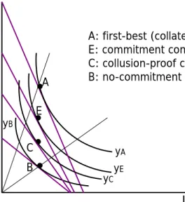
E: commitment contract with TC D: deviation contract B: no-commitment contract IN IK TC to give up to deviate yA A

.

.

Figure 4: The commitment role of trade credit.

Point E in Figure 4 depicts the input combination and the level of output corresponding to the commitment contract implied by Proposition 4. Point D represents the level of output obtained under deviation. Suppose that initially the entrepreneur signs the commitment contract and then decides to deviate. When he sees the entrepreneur altering the input provision, the supplier refuses to sell inputs on credit. This implies a decline in trade credit, hence in external financing, with a subsequent decline in the scale of production that makes deviation costly. By construction of the commitment contract, this decline is such that the entrepreneur is indifferent between sticking to the original contract and deviating. Graphically, points D and E lie on the same isoquant and thus involve the same level of output. The vertical distance between the isocost line intersecting point E and the one tangent to point D represents the amount of trade credit the entrepreneur has to give up to make the contract incentive-compatible. This guarantees that point E is the equilibrium outcome, i.e., the commitment contract.

This discussion implies that whether deviating from the original contract is profitable or not depends on the amount of trade credit the entrepreneur is getting under the original contract, which corresponds to the amount he has to forgo in case of deviation. It follows that the bank can always prevent deviation by reducing its supply of financing in such a way that the amount of trade credit the entrepreneur gives up by deviating reduces production so much as to make him prefer to honor the original contract. With more bank financing and less trade credit, the entrepreneur would still have an incentive to deviate, as the extra profits from altering the input combination would more than offset the lower investment due to lack of trade credit.

Notice that point E lies between point A (first-best) and point B (uncollateralized bank contract). The commitment contract cannot replicate the first-best, since the cheaper bank credit is partially replaced by more expensive trade credit. However, the commitment contract gives greater profits than the uncollateralized bank contract. By signaling that the bank loan will be used to purchase the inputs as specified, trade credit makes the collateralized bank contract available to the parties. The bank does not need to observe the firm-supplier contract. It can foresee the participation of the supplier in the venture and anticipate the commitment effect of trade credit, which arises from the fact that the supplier provides a share of the capital inputs on credit and has the right to a share of its collateral value in case of default. Both conditions have to be satisfied for the entrepreneur to have no incentive to alter the input mix ex-post.

Finally, since the commitment effect of trade credit allows the entrepreneur to access collateralized financing, point E has a more capital-intensive input combination than point B.

The foregoing analysis allows us to derive the following predictions:

Prediction 1. When investment is non-contractible, trade credit facilitates access to secured bank financing.

Prediction 2. Firms using trade credit and collateralized bank credit invest more intensively in pledgeable assets than firms using only uncollateralized bank credit.

4

Firm-supplier collusion

In Section 3, we argue that trade credit enables the firm to overcome its problem of commitment to the bank. This is because the supplier will always refuse to extend credit after observing the entrepreneur’s deviation, as he will fail to break even on the new input combination. Thus, the use of trade credit implicitly tells the bank that the entrepreneur is sticking to the original contract. However, the supplier might still be willing to extend credit even after detecting deviation, as long as the terms of the contract were renegotiated to allow him to at least break even. In this section, we extend the model to allow for collusive agreement between entrepreneur and supplier. Suppose that entrepreneur, bank and supplier have agreed on the contract terms described in Proposition 3, with γ =γ∗. Once the loan from the bank, L∗_B(γ∗) is obtained, the entrepreneur may then seek an agreement with the supplier to alter the input mix at the expense of the bank, i.e. to reduce the investment in capital and increase that in labor. If the supplier is to accept, they must renegotiate the contract terms, i.e. loan

size and repayments, so as to enable the supplier to at least break even:16

pRS+ (1−p) (1−γ)βIK ≥LS(γ)rS. (14)

If agreed, the new arrangement would allow an increase in overall profits at the expense of the bank. Any collusive rent - the difference between the returns under deviation and commitment - is then shared between entrepreneur and supplier. For simplicity, we assume that any collusion rent is seized by the entrepreneur.17

This allows us to define the gross collusion rent and describe its properties in Proposition 5.

Definition 2 Define ΠC(γ) as the profits from collusion for a generic γ solving programme PC in the Appendix andΠC(γ)−Π∗(γ)as the gross collusion rent, whereΠ∗(γ) are the profits from commitment as defined in Prop. 3 for a generic γ.

Proposition 5 The gross collusion rentΠC(γ)−Π∗(γ) is increasing inγ and is zero iffγ = 0.Thus, any collateralized firm-bank-supplier contract is vulnerable to collusion between firm and supplier at the expense of the bank.

Proposition 5 states that a collusive agreement to change the input combination ex-post, causing losses to the bank, is always profitable for entrepreneur and supplier. Thus, while incentive-compatible in the case of unilateral deviation, the commitment contract is not collusion-proof. The only way for the bank to stop the other parties from colluding, therefore, is to offer an unsecured contract (γ = 0). However, reaching a collusive agreement may be costly. This cost may be due to the time and effort spent in writing and enforcing the side contract, or to the risk of being prosecuted. It may also be the effect of reputational concerns.18 To capture this cost, defineα ∈[0,1] as the fraction of the profits from deviation that is lost in reaching such an agreement and [(1−α) ΠC(γ)−Π∗(γ)] as the net rent from collusion. This formulation enables us to find an interiorγ that stops parties from colluding. In particular, for a small cost of collusion the bank can always preclude it by restricting the set of contract offers to those that guarantee a non-positive collusion rent, i.e. those that satisfy the following constraint:

(1−α) ΠC(γ)−Π∗(γ)≤0 (15)

16_{An alternative agreement would keep the loan size fixed (L}∗

S(γ)) and alter only the repayments schedule. However,

while this would not alter the qualitative properties of the collusion-proof contract, there is no real reason to impose this constraint on the renegotiation. Moreover, renegotiating all the contract terms and not only repayment is profit-maximizing, as it gives the firm the possibility of reducing its reliance on costly trade credit.

17_{This is without loss of generality, as alternative distributions would not alter our qualitative results.} 18

Is the commitment contract collusion-proof when we measure the collusion rent net of bargaining costs? More specifically, at γ = γ∗ (the value of γ that ensures no unilateral incentive to deviate), is constraint (15) satisfied? The answer depends on the cost of collusion, α. Let us define α∗(γ∗) as the value of α at which the the collusion-proof condition (15) is satisfied with equality when γ =γ∗. Whenα≥α∗(γ∗), the value ofγ that solves (15) is greater thanγ∗,so that the commitment contract can also accommodate collusion. When α < α∗(γ∗), the value of γ that solves (15) is less than

γ∗ and the commitment contract is open to collusion. This amounts to saying that the value of γ

that accommodates both unilateral deviation and collusion has to solve the following global collusion proofness constraint:

max

(1−α) ΠC(γ),ΠD(γ) −Π∗(γ)≤0. (16) This allows us to state the result in Proposition (6):

Proposition 6 The set of collusion-proof bank contract offers hasγ = ˆγ(α)≤γ∗, whereγˆ(α)satisfies condition 16. The properties of the collusion-proof firm-bank-supplier contract are those described in Proposition 3, with γ = ˆγ(α).

Corollary 1 Under the collusion-proof contract, the share of inputs bought on credit is decreasing in the cost of collusion α, while the share of inputs paid for in cash, asset tangibility and expected profits are increasing in α.

The above analysis shows that the properties of the optimal contract depend on the cost of collusion. Three possible scenarios can arise. First, collusion can be so costly that it is never profitable:

α(γ∗) ≤ α ≤ 1. The rent from collusion is lower than the rent from deviation, so that the global collusion-proof condition (16) coincides with the incentive-compatibility condition (13). This case corresponds to the case already analyzed in Section 3: The entrepreneur buys commitment from the supplier through trade credit and takes a partially collateralized loan from the bank. The equilibrium is point E in Figure 5.

Second, collusion may be costly but profitable: 0< α < α(γ∗). The rent from collusion is greater than from deviation, so that the global collusion-proof condition (16) coincides with collusion proof condition (15). The bank can reduce the scope for collusion by further reducing its participation in the venture: its stake in the bad state the maximum share of the collateral to be liquidated -and the loan size both shrink. The lower the cost of collusion, the less the bank’s participation -and

the larger the amount of trade credit necessary to make the contract collusion-proof. The properties of the optimal contract are those described in Proposition 3 with γ = ˆγ(α). The equilibrium point corresponding to this case is represented by point C in Figure 5. This point is located between point E (commitment contract) and point B (uncollateralized bank contract), the exact position depending on the cost of collusion. The lower the cost, the further from point E and the closer to point B the new equilibrium is. Also, notice that a decrease in the cost of collusion that shifts the equilibrium from point E towards point B, also makes the input combination more labor-intensive, since the relative price ratio (capital/labor) decreases.

Lastly, collusion may be costless (α = 0). Entrepreneur and supplier can grab the entire surplus from their agreement. In this case, the only way for the bank to break even is by offering an unsecured credit contract. No longer having a stake in the firm’s bad state return, the bank is reimbursed only in the good state. This arrangement completely removes any incentive to collude. Trade credit can still be used, but only to exploit the liquidation ability of the supplier, not to buy commitment. In this case, the supplier finances and liquidates the full collateral value of the capital inputβIK.19

.

.

B: no-commitment contract (un-collateralized BC)

IN IK yA A

.

.

Figure 5: The collusion-proof contract.

19

We are implicitly assuming here thatrS < r_pB, i.e. that Assumption 1 holds with strict inequality when γ = 0.

In this case, the equilibrium point will still be located away from point B and to its right. The entrepreneur can at least pledge some collateral to the supplier, therefore improving on the case in which only uncollateralized bank credit is available (point B). IfrS= r_pB, the entrepreneur is indifferent between taking trade credit only or a mix of trade and

bank credit. The benefit of pledging inputs to the supplier is fully offset by the higher cost of trade over bank credit. The equilibrium point corresponding to this case is point B.

5

Testable Predictions

This section uses the analysis developed in Sections 3 and 4 to identify new testable predictions on how firms’ investment and financing decisions vary across sectors and markets. Specifically, Subsection 5.1 exploits cross-sectional differences in input characteristics such as liquidity and substitutability, and Subsection 5.2 focuses on differences in the cost of collusion.

5.1 The commitment problem in the cross-section of firms

In our model, trade credit solves the commitment problem between bank and entrepreneur and restores the benefits of collateral, which can be defined as the difference between the entrepreneur’s profits under the commitment and under the unsecured contract. Entrepreneur’s profits under commitment are increasing in input liquidity, β, as shown in Proposition 3. Profits under the unsecured contract do not depend on input liquidity, since assets are not pledged. Thus the benefits of trade credit are greater the greater input liquidity is. To some extent, input liquidity reflects industry characteristics. For example, standardized goods are likely to have more scrap value than differentiated products or services. Thus, firms using standardized products are more likely to take trade credit to access secured bank financing. This allows the following prediction:

Prediction 3. Firms buying standardized inputs are more likely to use collateralized bank and trade credit than firms buying differentiated inputs or services.

A second important characteristic of the inputs is degree of substitutability. The commitment problem arises because the entrepreneur can change the input combination after the loan has been granted. For trade credit to play a role as a commitment device, then, it is crucial that the project uses inputs that are at least partially substitutes. The higher the degree of substitutability between inputs, the more severe the commitment problem between entrepreneur and bank and the more valuable trade credit is. In the extreme case where inputs are used in fixed proportions, there is no extra-profit to be gained by changing the input combination. Since there is no incentive to deviate, the entrepreneur has access to collateralized bank financing with no need to take trade credit. Thus, we get the following prediction:

Prediction 4. Firms with a higher degree of substitutability between inputs are more likely to use collateralized bank and trade credit.

5.2 Firm decisions and the cost of collusion

From Proposition 6 and Corollary 1, the properties of the financial contracts with bank and supplier depend on the cost of reaching a collusive agreement. In this section, we inquire more thoroughly into the relation between cost of collusion, optimal financing contracts (including not only the amount of bank and trade credit but also the specific type of contract (secured/unsecured)) and investment decisions. Figure 6 summarizes the use of trade and bank credit and the level of output for different levels of collusion costs.

Costly collusion Medium-cost collusion

Costless collusion Trade credit

- share of capital inputs

bought on credit Independent of α Decreasing in α

Bank credit

- share of icapital inputs

bought on cash , increasing in α

- type on contract Collateralized (γ=γ*) Collateralized (0<γ<γ*) Uncollateralized (γ=0) Output level Point E Point C Close to point B

0 = α *) ( 0<α<αγ ) 1 ( −β β α γ*( )] 1 [ − 1 *) (γ ≤α≤ α β γ*) 1 ( − β β γ* γ*(α)β

Figure 6: Financing and investment decisions when the cost of collusion varies.

In our setting it is optimal to take the smallest possible amount of trade credit that still guarantees a credible commitment. The first line of Figure 6 shows the share of capital inputs bought on account,

LS/IK for different levels ofα. If the cost of collusion is sufficiently high, α∗(γ∗)≤α≤1, this share

is equal to the scrap value of inputsβ multiplied by the share of collateral accruing to the supplier in case of default under the commitment contract, 1−γ∗, and is thus independent of α. When the cost of collusion falls below α∗(γ∗) and keeps decreasing, the share of inputs bought on credit increases since the entrepreneur needs to increase the supplier’s stake in the venture, 1−γ∗(α), to credibly signal commitment to the bank. In the extreme case of costless collusion (α = 0), entrepreneur and supplier always cheat at the expense of the bank. Thus, the bank only offers an uncollateralized credit contract. The firm still uses trade credit, but only in order to exploit the liquidation technology of the supplier in case of default, not as a commitment device. The share of capital inputs bought on credit reaches its maximum, namely the collateral value of the inputβ.

The pattern of the share of capital inputs paid for in cash (through bank credit) is the mirror image of that bought on account; it is described in the second line of Figure 6. The share is equal to

the scrap value of inputs, β, multiplied by the fraction of the collateral value accruing to the bank in case of default, γ. The share of input paid for in cash is constant for any α ≥ α∗(γ∗) and decreases when the cost of collusion decreases below α∗(γ∗, since the bank needs to reduce its stake in order to avoid collusion. For any positive cost of collusion, the bank offers a collateralized contract. When

α= 0, the bank only offers an unsecured loan, which is used to finance (1−β) of the tangible inputs and all the intangibles.

If we define the benefit of trade credit as the difference between the entrepreneur’s profits under the collusion-proof contract and under the no-commitment contract, these benefits are shown to be greater, the lower the cost of collusion. Figure 5 gives an indication of how profits change for different costs of collusion. In particular, for any α∗(γ∗) ≤ α ≤ 1, the equilibrium is point E, very far from point B. Here the benefits of trade credit are greatest. When the cost of collusion falls belowα∗(γ∗), the equilibrium is represented by point C, which gets closer to point B the easier it is to collude. In the extreme situation in which collusion is costless, the benefits are low or nil, depending on whether it is still profitable to use trade credit for its liquidation value. The equilibrium is located at or very close to B.

Finally, notice that at different production levels correspond different degrees of input tangibility as represented in Fig. 5. For any α∗(γ∗) ≤ α ≤ 1, the degree of input tangibility is greater than 1, independent of α and represented by the slope of the expansion path running through point E. The input combination is biased towards capital inputs due to the lower financing cost implied by their collateral value. When the cost of collusion falls below α∗(γ∗), input tangibility decreases, as shown by the slope of the expansion path running through point C. The lower the cost of collusion, the further down the equilibrium point C will be, and the lower the degree of input tangibility. In the extreme case of costless collusion, if we assume that the actual costs of trade and bank credit are equal (rS = r_pB), the degree of input tangibility is 1 (slope of the expansion path through point B).

The foregoing discussion allows us to get the following predictions:

Prediction 5. The share of inputs bought on account is decreasing in the cost of collusion.

Prediction 6. The share of inputs paid for in cash, through bank credit, is increasing in the cost of collusion.

Prediction 7. The benefits of using trade credit are larger, the costlier it is to collude.

Prediction 8. Firms use technologies more intensive in tangible assets the costlier it is to collude.

and enforcing a side contract, which in turn may depend on the strength of the firm-supplier relation. For example, if the firm in our story is an important customer of the supplier, the time and effort spent in convincing the supplier to accept the collusive contract should be not too high. The firm becomes an important customer when it is the only buyer of the good produced by the supplier or if the good supplied is customized i.e., made to the customer’s unique specification. In this case, the supplier cannot easily resell the good to a different buyer. The opposite argument holds if the product is standardized, or if the market structure of the product is very competitive i.e., there are many potential customers for the good sold by the supplier. Restated, Predictions 5 to 8 could identify relations between the financing and investment decisions on the one hand and product characteristics on the other hand. These predictions are still empirically unexplored.

6

Discussion

Here we discuss the robustness of our theoretical setting. Subsection 6.1 investigates whether alternative bank contracts could solve the commitment problem. Subsection 6.2 focuses on the degree of information-sharing between supplier and bank. Subsection 6.3 discusses the assumption of the exclusive lending relation. Subsection 6.4 questions the role of the supplier as an informed lender and provides alternative interpretations. Subsection 6.5 discusses the seniority rule implied by the optimal contract.

6.1 Can alternative bank contracts solve the commitment problem?

In the previous sections, we have shown three main points. First, any even partially collateralized bank contract is plagued by a commitment problem that makes it non-viable. Second, the uncollateralized contract removes this problem but also eliminates the benefits of collateralizing inputs. Third, the commitment problem can be overcome without forgoing the benefits of collateralized bank loan by involving the supplier in the lending relation. In this section, we investigate whether alternative contracts can solve the commitment problem.

In our setting, the entrepreneur has an incentive to change the input combination after the loan has been made because the ex-ante input price ratio is different from the ex-post, the difference being the collateral value of capital inputs. It follows that a contract in which inputs are not pledged to creditors in case of default but are seized by the entrepreneur, and the bank gets paid only in the good state, would completely realign the entrepreneur’s incentives, by making the ex-ante and ex-post

input prices equal. The optimization problem corresponding to this contract would be the same as with investment observability (see the benchmark case in Section 2). The crucial question here is whether this contract is viable or not. In practice, when a firm is unable to repay its creditors, it can call for the bankruptcy stay. Any legal system automatically requires that all assets still in place be kept away from the entrepreneur and used to repay creditors following a scale of priority that depends on the specific characteristics of the contract. Thus, in practice the firm’s assets are also used to repay unsecured claims. It follows that even if the bank contract is not secured, the assets are usedde facto

to repay the bank. To conclude, an agreement providing that in case of default all assets in place be seized by the entrepreneur, although contractually optimal, is overcome by the actual provisions of the legal system.20

Alternatively, one could argue that there is no need to use trade credit if the bank can condition financing on the number of employees. This could work as a commitment device if the deviation consisted in cutting the number of employees ex-post and labor market rules did not allow workers to be easily fired. However, in our setting the entrepreneur has an incentive to increase (rather than reduce) the number of employees, and this can be easily done in any labor market.

Finally, the literature on risk-shifting has investigated asset substitution in a context of conflict of interest between shareholders and bondholders. This literature has also identified instruments that can mitigate this problem. One might then wonder whether these instruments could help solve our commitment problem as well. Smith and Warner (1979), among others, show that some kinds of asset substitution problems that induce excess risk-taking can be mitigated by loan covenants that constrain investment or financing decisions. In our context, debt covenants that specify the investment projects the firm is allowed to undertake, as by requiring the manager to accept only projects with a given combination of inputs, could solve the commitment problem. Debt covenants are in fact widespread, but the constraints generally do not specifically limit investment policy, possibly because they would be expensive to enforce. Rather they restrict the firm’s financial investment, the disposition of assets and the firm’s merger activity.

Green (1984) shows that the risk-shifting problem can be mitigated by resorting to convertible debt. Besides the fact that there is no unanimity on the properties of convertible debt contracts, the theoretical setting and the predictions of the literature on risk-shifting are very different from ours.21

20_{One could assume that the entrepreneur could hide these assets and resell them before the bankruptcy procedure}

starts. This would again realign incentives, but only if all the assets were diverted. If instead only a share were diverted, the incentive to deviate would still remain.

21

In this literature, the asset substitution problem plagues a pure (uncollateralized) debt contract, owing to conflicts of interest between shareholders and bondholders. In our model, there are no conflicts of interest when the project is financed with a pure debt contract. It is the use of collateral that introduces an asset substitution problem. This difference is crucial and means that the convertible debt contract is not a viable instrument to solve our commitment problem.

6.2 How much information-sharing between financiers?

As we have seen, trade credit can signal the entrepreneur’s willingness to abide by the ex-ante efficient bank contract. When the bank gets this signal, it offers a collateralized loan. Does our story imply that the bank needs to observe the amount of trade credit taken or even the full properties of the supplier-entrepreneur contract? How much information-sharing between bank and supplier is needed to access a collateralized bank loan?

In our model, the bank only needs to know that there is some supplier willing to lend money to the entrepreneur. All the other relevant information, including the specific amount of trade credit offered can be inferred by solving the entrepreneur’s optimization problem. The intuition is as follows. In period t = 1, bank and supplier offer a menu of incentive-compatible contracts (see the time-line in Figure 1). Each contract offer solves the entrepreneur’s optimization problem for any given combination of bank and trade credit.22 The entrepreneur then chooses the contract that minimizes the total cost of external financing. Thus, from the choice of a given bank contract, the bank immediately infers how much trade credit will be taken by the entrepreneur as well as the repayment to the supplier in the good and in the bad state.

While the degree of information-sharing assumed in our setting is small, ample anecdotal evidence suggests that in considering a loan application banks usually ask for financial information and for balance-sheet data, including accounts payable (Garcia-Appendini, 2010). In addition, banks may have access to valuable information about trade credit through credit bureaus. For example, the firm’s trade credit payment history is routinely included in the credit reports provided by credit bureaus or business information exchanges such as the Dun & Bradstreet (Kallberg and Udell 2003). This evidence suggests that in practice banks are likely to have more information about suppliers’ payment practices than our model implies.

to its perceived role, can produce shareholders’ risk-shifting incentives.

22

Contracts merely satisfying the bank’s participation constraint would not be incentive-compatible for the entrepreneur and so are not offered.

6.3 Exclusive lending relations

In Section 1 we have assumed that the entrepreneur has exclusive lending relations with bank and supplier. Is exclusivity a necessary condition? What happens if the entrepreneur buys inputs from several suppliers? In this case, the optimal contract implies that each supplier loan is tied closely to the amount of inputs provided by that supplier, not to the total amount of inputs. Thus, each supplier only observes his own fraction of the input purchases. Unless we assume some sort of information-sharing among suppliers, no supplier actually knows whether the ex-ante optimal input combination has been purchased. Thus, the entrepreneur cannot be prevented from deviating and trade credit no longer solves the commitment problem.

To get this intuition, suppose that the optimal input combination requires 10 units of capital and 8 workers. The amount of trade credit that would remove the entrepreneur’s incentive to deviate is 6, and the bank is willing to finance the rest (4 units of capital plus the 8 workers). If there is only one supplier, our story works. But suppose there are two suppliers: one selling 6 units of capital on credit and having the right to 10% of the collateral value of these inputs in case of default; the other selling 4 inputs in cash. Rather than abiding by the efficient contract, the entrepreneur could take just the 6 units on credit from the first supplier and use the loan of 4 from the bank to hire workers rather than buy the remaining 4 units of capital. The supplier would not be aware of the deviation and would still break even. But the bank would get negative expected profits, since the total collateral value would be less than expected. Anticipating the entrepreneur’s deviation, the bank would never offer a collateralized contract. That is, with more than one supplier trade credit no longer works as a commitment device, since its provider would be unable to detect and avoid deviation.

Similar reasoning applies to the bank lending relation. With several banks, the aggregate credit obtained from all the banks could be larger than the incentive-compatible amount, giving the entrepreneur an incentive to deviate. Anticipating this, each bank would offer an uncollateralized contract and trade credit would play no commitment role. Thus, here too exclusivity in the lending relation is necessary, unless we assume information-sharing among banks such that each knows the amount lent by all the other banks involved in the project.

6.4 Is the supplier the only informed lender?

In our analysis, we assume that the more costly, informed lender is the supplier and the cheaper, uninformed financier is the bank. Other interpretations are possible, however. We could assume that