Probabilistic topographic information visualisation

Some pages of this thesis may have been removed for copyright restrictions.

Probabilistic Topographic Information

Visualisation

I

AIN

T

IMOTHY

R

ICE

Doctor Of Philosophy

ASTON

UNIVERSITY

June 2015

c

Iain Timothy Rice, 2015

Iain Timothy Rice asserts his moral right to be identified as the

author of this thesis

This copy of the thesis has been supplied on condition that anyone who

consults it is understood to recognise that its copyright rests with its author

and that no quotation from the thesis and no information derived from it

may be published without appropriate permission or acknowledgement.

A

STON

U

NIVERSITY

Probabilistic Topographic Information

Visualisation

I

AIN

T

IMOTHY

R

ICE

Doctor Of Philosophy, 2015

Report Summary

The focus of this thesis is the extension of topographic visualisation mappings to al-low for the incorporation of uncertainty. Few visualisation algorithms in the literature are capable of mapping uncertain data with fewer able to represent observation uncertainties in visualisations. As such, modifications are made to NeuroScale, Locally Linear Em-bedding, Isomap and Laplacian Eigenmaps to incorporate uncertainty in the observation and visualisation spaces. The proposed mappings are then called Normally-distributed NeuroScale (N-NS), T-distributed NeuroScale (T-NS), Probabilistic LLE (PLLE), Prob-abilistic Isomap (PIso) and ProbProb-abilistic Weighted Neighbourhood Mapping (PWNM). These algorithms generate a probabilistic visualisation space with each latent visualised point transformed to a multivariate Gaussian or T-distribution, using a feed-forward RBF network.

Two types of uncertainty are then characterised dependent on the data and mapping procedure. Data dependent uncertainty is the inherent observation uncertainty. Whereas, mapping uncertainty is defined by the Fisher Information of a visualised distribution. This indicates how well the data has been interpolated, offering a level of ‘surprise’ for each observation.

These new probabilistic mappings are tested on three datasets of vectorial observa-tions and three datasets of real world time series observaobserva-tions for anomaly detection. In order to visualise the time series data, a method for analysing observed signals and noise distributions, Residual Modelling, is introduced.

The performance of the new algorithms on the tested datasets is compared qualita-tively with the latent space generated by the Gaussian Process Latent Variable Model (GPLVM). A quantitative comparison using existing evaluation measures from the litera-ture allows performance of each mapping function to be compared.

Finally, the mapping uncertainty measure is combined with NeuroScale to build a deep learning classifier, the Cascading RBF. This new structure is tested on the MNist dataset achieving world record performance whilst avoiding the flaws seen in other Deep Learning Machines.

Contents

2.2.1 The PCA/MDS Mapping . . . 20

2.2.2 Locally Linear Embedding . . . 23

2.2.3 Sammon Mapping & NeuroScale . . . 27

2.3 Graph Distance Mappings . . . 30

2.3.1 IsoMap . . . 30

2.3.2 Laplacian Eigenmaps . . . 33

2.4 Latent Variable Models . . . 35

2.4.1 Generative Topographic Mapping . . . 36

2.4.2 Gaussian Process Latent Variable Model . . . 40

2.5 Quality Criterion . . . 44

2.5.1 Rank . . . 44

2.5.2 Trustworthiness and Continuity . . . 44

2.5.3 Mean Relative Rank Error . . . 46

2.5.4 Local Continuity Meta-Criterion . . . 47

2.5.5 Quality of Open Box embeddings . . . 47

2.6 Conclusion . . . 50

3 Incorporating Observation Uncertainty into Visualisations 52 3.1 Introduction . . . 52

3.2 Current approaches to uncertainty mappings . . . 53

3.2.1 Probabilistic NeuroScale . . . 54

3.2.2 Geometry of hyperspheres . . . 55

3.2.3 Geometry of hyper-ellipsoids . . . 56

3.3 Elliptical Gaussian Probabilistic NeuroScale - N-NS . . . 58

3.4 Elliptical T-distributed NeuroScale - T-NS . . . 61

3.4.1 Shadow Targets for T-NS . . . 64

3.5 Probabilistic Locally Linear Embedding - PLLE . . . 66

3.6 Probabilistic Isomap - PIso . . . 70

3.7 Probabilistic extension to Laplacian Eigenmaps - PWNM . . . 71

CONTENTS

4 Interpreting Uncertainties In Visualisations 74

4.1 Introduction . . . 74

4.2 Uncertainty Surfaces . . . 75

4.2.1 Similarities with GTM and GPLVM . . . 76

4.3 Mapping Uncertainty . . . 77

4.4 Feed Forward Visualisation Mappings . . . 82

4.4.1 RBF PLLE . . . 82

4.4.2 RBF PWNM . . . 84

4.4.3 RBF PIso . . . 85

4.4.4 Mapping Uncertainty with T-NS . . . 87

4.5 Conclusion . . . 87

5 Visualisation of Vectorial Observations 89 5.1 Introduction . . . 89

5.2 MNist Dataset . . . 91

5.3 Four Clusters Dataset . . . 99

5.4 Punctured Sphere Dataset . . . 105

5.5 Overview . . . 112

6 Visualisation of Time Series: The Method of Residual Modelling 116 6.1 Introduction . . . 116

6.2 Residual Modelling . . . 117

6.3 Univariate Time Series: Dutch Power Data . . . 121

6.4 Multivariate Time Series: EEG Seizure data . . . 127

6.5 Univariate Time Series & Noise Model: SONAR dataset . . . 136

6.6 Overview . . . 148 7 Cascading RBFs 150 7.1 Introduction . . . 150 7.2 Background . . . 151 7.2.1 Deep MLPs . . . 151 7.2.2 Convnets . . . 153 7.2.3 Issues . . . 154 7.3 The Cascading RBF . . . 155 7.3.1 The Process . . . 155

7.3.2 The Test: MNist . . . 159

7.3.3 Unstable Functions . . . 160 7.3.4 Unreliable Mappings . . . 163 7.4 Overview . . . 165 8 Conclusions 166 8.1 Review Of Thesis . . . 166 8.2 Contributions . . . 168 8.3 Future Work . . . 168

CONTENTS

B Non-Topographic Visualisation Mappings 185

B.1 Introduction . . . 185

B.2 T-SNE . . . 186

B.3 AutoEncoder . . . 191

B.4 Deep Gaussian Process . . . 191

C Optimisation of GTM 193 D Derivation of Fisher Information 196 E Gradients for SONAR Noise Model 199 E.1 The Model . . . 201

E.2 The Gradients . . . 203

List of Figures

2.1 Visualisation algorithms taxonomy diagram . . . 18

2.2 3-dimensional plot of the Open Box dataset. . . 20

2.3 Open box embedded by PCA/MDS. . . 24

2.4 Open box embedded by LLE. . . 27

2.5 Open box embedded by Sammon mapping. . . 28

2.6 Open box embedded by Isomap using four neighbours. . . 32

2.7 Open box embedded by Isomap with eight neighbours. . . 33

2.8 Open box embedded by Laplacian Eigenmapping with four neighbours. . 35

2.9 Open box embedded by GTM. . . 38

2.10 Open box embedded by GTM with points superimposed upon the magni-fication factors. . . 39

2.11 Open box embedded by GPLVM with back constraints. . . 42

2.12 Open box embedded by GPLVM with back constraints with posterior probability surface shown. . . 43

2.13 Quality criterion for visualisations of the Open Box dataset . . . 48

5.1 Examples of nine images taken from the MNist dataset (left) and his-togram of dissimilarities (right). . . 91

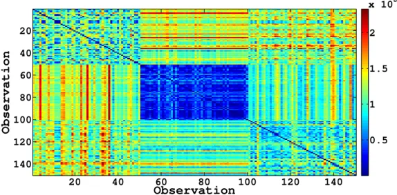
5.2 Dissimilarity matrix for 150 sample subset of the MNist database incor-porating uncertainty. . . 92

5.3 Sammon mapping for 150 samples from the MNist database accounting for uncertanties in observations. . . 93

5.4 Visualisations of the MNist dataset using N-NS, T-NS and PLLE . . . 94

5.5 Visualisations of the MNist dataset using PIso, PWNM and GPLVM . . . 95

5.6 Quality criteria for the probabilistic MNist visualisations. . . 97

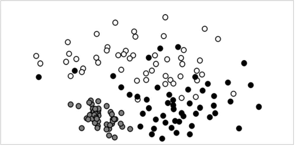
5.7 Plot of the four clusters dataset and histogram of dissimilarities. . . 99

5.8 Dissimilarity matrix for four clusters dataset. . . 100

5.9 Visualisations of the four clusters dataset using N-NS, T-NS and PLLE . . 102

5.10 Visualisations of the four clusters dataset using PIso, PWNM and GPLVM 103 5.11 Quality criterion for visualisations of the four clusters dataset . . . 104

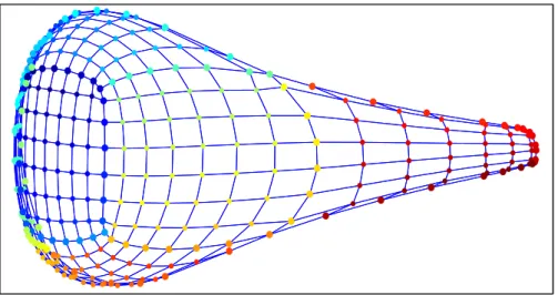
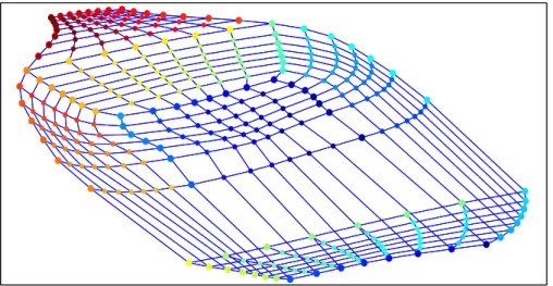
5.12 Plot of the Punctured Sphere dataset and histogram of dissimilarities. . . . 106

5.13 Dissimilarity matrix for the uncertain punctured sphere dataset. . . 107

5.14 Visualisations of the uncertain punctured sphere dataset using N-NS, T-NS and PLLE. . . 108

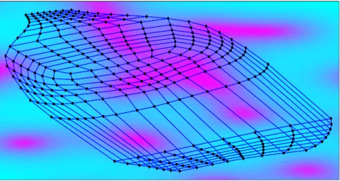
5.15 Visualisations of the uncertain punctured sphere dataset using PIso, PWNM and GPLVM. . . 109

5.16 T-NS mapping of the uncertain punctured sphere dataset withν=35. . . 112

LIST OF FIGURES

6.1 Sample of the Dutch Power dataset and histogram of dissimilarities. . . . 121

6.2 Nonlinear PACF and residuals for the Dutch Power dataset . . . 122

6.3 α-βplot for the Dutch Power dataset . . . 123

6.4 Dissimilarity matrix for the Dutch Power dataset . . . 124

6.5 Visualisations of the Dutch data using N-NS, T-NS and PLLE. . . 125

6.6 Visualisations of the Dutch data using PIso, PWNM and GPLVM. . . 126

6.7 Quality criterion for visualisations of the Dutch Power dataset . . . 128

6.8 Sample of the EEG dataset and histogram of dissimilarities. . . 129

6.9 Nonlinear PACF errors for the EEG dataset. . . 130

6.10 Dissimilarity matrix for the EEG dataset. . . 131

6.11 Visualisations of the EEG data using N-NS, T-NS and PLLE. . . 132

6.12 Visualisations of the EEG data using PIso, PWNM and GPLVM. . . 133

6.13 Quality criterion for visualisations of the EEG dataset . . . 135

6.14 Signal energy and histogram of dissimilarities for the SONAR dataset. . . 138

6.15 Nonlinear PACF and residuals for the SONAR dataset. . . 139

6.16 Negative log-likelihoods for the mixture model fit to the SONAR dataset. 140 6.17 Mixture weights for the mixture model fit to the SONAR dataset. . . 141

6.18 Dissimilarity matrix for the SONAR dataset. . . 143

6.19 Visualisations of the SONAR data using N-NS, T-NS and PLLE. . . 144

6.20 Visualisations of the SONAR data using PIso, PWNM and GPLVM. . . . 145

6.21 Quality criterion for visualisations of the SONAR dataset. . . 147

7.1 Training procedure for deep MLPs. . . 152

7.2 Adversarial example used to cause misclassification in a Convnet. . . 154

7.3 Schematic for a three layer cascading RBF. . . 156

7.4 Schematic for a three layer Cascading RBF used on MNist dataset. . . 159

7.5 Test of adversarial examples against a Cascading RBF. . . 162

7.6 Histogram of mapping uncertainties for the trained, test and random im-ages for the MNist dataset Cascading RBF. . . 164

B.1 Open box embedded by T-SNE. . . 188

B.2 Quality criterion for the T-SNE and Sammon mappings of the Open Box dataset. . . 189

B.3 T-SNE and Sammon mapping visualisations of a randomly generated 2-dimensional dataset embedded in 3-2-dimensional space. . . 190

List of Tables

2.1 STRESS measures for Open Box mappings. . . 50 3.1 Comparison of cost functions from standard methods with proposed

al-gorithms. . . 73 5.1 Best and worst performance of visualisation quality criterion for vectorial

datasets . . . 114 6.1 Comparison of mapping quality criteria for time series datasets. . . 148 7.1 Misclassification rates for several leading MNist classification methods. . 161

List of Frequently Used Symbols

xi Theith observation vector

ti The target corresponding to observationi

yi Theith visualised vector corresponding to observationXi

Γ The Gamma function

Λ The diagonal matrix of eigenvalues in descending order φ Nonlinear function or functional

φφφi The nonlinear vector given byφ d(Xi,Cj)

Φ The matrix set ofφφφivectors of dimensionsN×M

Ψ The Digamma function Σ A covariance matrix

A† The Moore-Penrose pseudo-inverse of a matrixA Cj The jthcentre of an RBF network

D A squareN×N dissimilarity matrix where thei jth element is given byd(i,j) d(i,j) A pairwise dissimilarity measure between observations or latent pointsiand j.

d_x(i,j) The dissimilarity between observationsiand j d_y(i,j) The dissimilarity between visualised pointsiand j E_x The expectation overx

I_O×P An augmented Identity matrix of the firstPcolumns of the Identity matrixI_O IP The Identity matrix of dimensionsP×P

M The number of centres,C_j, in an RBF network

N The number of observations

p(z) The probability distribution overz

S An observed or estimated covariance matrix

LIST OF TABLES

W A weight matrix

X The set of all observationsX_i. In the case whereX_iis a vector,xi,X is a matrix of

dimensionsN×O.

X∗ A new, unseen observation

X_t−m:t A delay matrix of observations from timet−mto timet (current)

Y The matrix set of visualised pointsyiof dimensionsN×P

RO Set of real numbers in observation dimension,O RP Set of real numbers in latent / visualised dimension,P

N

Acknowledgements

First and foremost I am grateful to my supervisor Professor David Lowe for all of the support, guidance and encouragement I have received throughout my time at Aston.

I wish to thank Thales, EPSRC and the KTN for their financial support which has allowed me to complete my PhD. I am particularly thankful to Les Hart, Rob Taylor, Geoff Williams, David Allwright and Roger Benton for their support on what has been an entirely different collaboration project for Thales.

Throughout my PhD studies I have received the strongest support from my wife Becky and son Ryan, as well as from my parents Joe and Joyce and from Tina and Shaun, without whom this work would not have been possible.

1

Introduction

‘If people do not believe that mathematics is simple, it is only because they do not realise how

complicated life is.’

- John von Neumann

1.1

Motivation

The work in this thesis stems from the inescapable fact that real world data is, in some way or another, uncertain. Data uncertainties are typically characterised as the result of the observation, measurement or analysis frameworks. Moreover, the data we are often most interested in is complex and, in the case it is vectorial, high dimensional.

Non-vectorial data poses its own set of unique problems. With these elements coupled it makes the task of understanding and generating reliable conclusions from data a difficult task. The mathematical analysis performed on such data typically conforms to the

Chapter 1 INTRODUCTION

general supervised regression or classification framework, involving a mapping from data observations to a set of targets. These scenarios have dominated research in pattern analysis over the past fifty years, [1],[2],[3].

Sometimes, however, there don’t exist any targets to map the data to. In this case one approach is to use summary statistics as a descriptor for data, or some feature-based representation of the data. An alternative, and often more useful analysis tool, is to generate a low-dimensional visualisation space, allowing for human interpretation of the data. The ability of humans in deciphering patterns in data, taking into account expertise, historical information or additional information not characterised in observations can surpass that of automated systems. Mapping observed data to a space where it can be visually interpreted relies on a visualisation algorithm. The ‘optimum’ positions of data observations in this (typically 2 or 3-dimensional) visualisation space depends on the algorithm being used. In general, the aim of such a mapping algorithm is to preserve global or local data structure, in which case they are called ‘topographic’. A prominent issue in the field of data visualisation is that many algorithms, for instance Locally Linear Embedding [4] or Isomap [5], suffer in quality when data is noisy, or uncertain. In addition to this there are often assumptions made as to the underlying manifold on which observations sit. These deficiencies presents a significant problem for real world data analysis.

In order to tackle the data uncertainty problem, this thesis extends current algorithms to incorporate inherent observation uncertainty and the uncertainty imposed by the

mapping from observation to visualisation space. A framework for representing these uncertainties in visualisations is also introduced, allowing for an informative

visualisation of data. Finally it is shown that the benefits of a thorough approach to manifold leaning, through topographic mapping, extends beyond data visualisation to areas such as deep learning classifiers.

Chapter 1 INTRODUCTION

1.2

Contributions

In this thesis a probabilistic framework is outlined for topographic information visualisation accounting for uncertainty. Specifically:

• Probabilistic extensions to NeuroScale, Locally Linear Embedding, Isomap and Laplacian Eigenmaps are introduced, accounting for observation uncertainty, allowing for feed-forward projection of new data.

• A framework for interpreting observation uncertainty and the imposed mapping uncertanty in visualisation spaces is outlined.

• A novel method for detecting anomalies in time series data using topographic visualisation is described.

• A new form of deep learning machine consisting of topographically pre-trained RBF networks is implemented in a classification setting.

1.3

Thesis Organisation

Chapter 2 offers an introductory background to some of the popular methods for

visualising data. Three criteria for quantitatively analysing visualisation performance are also outlined. Chapter 3 extends the deterministic mappings outlined in chapter 2 to allow for observation uncertainty. Chapter 4 proposes a method for representing both the uncertainties generated by observations and the visualisation mapping itself. Chapter 5 implements the methods of chapters 3 and 4 on three vectorial datasets, accounting for data uncertainty. In chapter 6 a process for visualising anomalies in time series data is introduced and demonstrated on three datasets. Chapter 7 combines topographic mapping with a deep learning machine in a classification setting. Finally, chapter 8 concludes the thesis.

2

Background

‘A mathematician is a device which turns coffee into theorems.’

- Alfred Rényi

2.1

Data Visualisation

This chapter forms an introductory section for the thesis describing the tools used for visualisation of data.

Firstly, the notion of visualisation must be described in terms of some data. The simplest and most intuitive case being where the data consists of a set of vectors. A few popular visualisation mechanisms require the data to be of this form (for instance [6], [7] and [8]). The purpose of a visualisation algorithm in this case is to reduce the dimensionality of these vectors such that the observations,x∈_RO_{, are mapped by some function to a}

Chapter 2 BACKGROUND

so that the new points,y, can be visually interpreted.

Many other visualisation algorithms do not require pointwise observations and can construct a visualisation space with only relative pairwise dissimilarities, in the form of a dissimilarity matrix,D, as inputs, the most commonly used being the Sammon map [9]. This allows for perceptual analysis of more abstract notions than data-points; for

instance, in visualising different time series, probability distributions or graphs. This is a significant benefit since these notions cannot be properly characterised by an observed vector point.

2.1.1

Methods

As with all areas of Machine Learning, there exist multiple different methods for construction of the functional mappings which generate a visualisation space. Each of these offer different results depending on the data and mapping parameters. These methods can be split into 3 groups:

1. Dissimilarity Mappings (section 2.2) 2. Graph Distance Mappings (section 2.3) 3. Latent Variable Models (section 2.4)

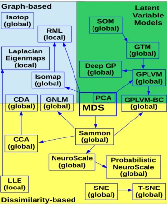
A taxonomy diagram showing examples of visualisation algorithms conforming to these groups and their links is shown in figure 2.1. Some of these algorithms are not included in this thesis but are shown for completeness. The Geodesic Nonlinear Mapping

(GNLM) [10] is a special case of the Sammon map with Geodesic dissimilarities, but the Sammon map in general does not specify the input dissimilarity; so GNLM is not

discussed in this thesis. Curvilinear Component Analysis (CCA) [11], and also

Curvilinear Distance Analysis (CDA) [12], extnsions to the Sammon map (and GNLM) requiring the specification of a neighbourhood weighting function and, for many popular function choices have little global impact on the visualisations generated. As such these are not discussed in this thesis. The Deep GP [13] and T-SNE [14] are not topographic,

Chapter 2 BACKGROUND Graph-based Dissimilarity-based Latent Variable Models MDS Isotop (global) PCA Isomap (global) Laplacian Eigenmaps (local) RML (local) SOM (global) GTM (global) GPLVM (global) GPLVM-BC (global) Deep GP (global) LLE (local) SNE

(global) (global)T-SNE Sammon

(global) NeuroScale

(global) Probabilistic _NeuroScale (global) CCA

(global) CDA

(global) (global)GNLM

Figure 2.1: Taxonomy diagram showing the grouping and links between popular visuali-sation algorithms. Arrows indicate a connection between algorithms, with arrows show-ing extensions to previous techniques. Most algorithms can be shown to be extensions to, or reliant upon, Multidimensional Scaling (MDS), of which PCA is a special case. but it may not be clear initially why and as such are included in Appendix B.

Riemannian Manifold Learning (RML) [15] is a principled local approach to manifold learning with impressive results. It does, however, require a background in Differential Geometry and is thus outside the scope of this thesis. Isotop [16] is an altogether different method for generating data visualisations, again with impressive mapping performance [17]. Despite this there is no clear cost function or knowledge of how it generates these visualisations and as such is not included in this thesis.

Firstly, Principal Component Analysis (PCA) [6] will be discussed in section 2.2. It will be shown that since it is a special case of metric Multidimensional Scaling (MDS) [18], it can be thought of as a dissimilarity-based mapping. Following this Locally Linear Embedding (LLE) [4] and Sammon mapping [9] will be introduced. These methods reconstruct observations by attempting to preserve the relative dissimilarities between the observations. Graph distance mappings including Isomap [5] and Laplacian

Chapter 2 BACKGROUND

and preserve the graph distances when generating visualised points. Latent Variable models such as Generative Topographic Mapping (GTM) [7] and the Gaussian Process Latent Variable Model (GPLVM) [8] attempt to define the most likely latent visualisation space which generates the observation space. These methods impose specific restrictions on the latent space and require observations to be pointwise vectors. The figures

generated in this thesis rely upon Matlab toolboxes for their implementation. The list below shows the algorithms and their relevant toolboxes:

• PCA/MDS, Isomap, LLE, Sammon Mapping, LE - drtoolbox [20],

• GTM, NeuroScale - Netlab toolbox [21],

• GPLVM - GPMat toolbox [22].

These toolboxes are widely used and thus considered robust for analysis in this thesis. In order to gain insight into the differences between the algorithms, and to later introduce mapping performance criteria, a comparison dataset will be used for

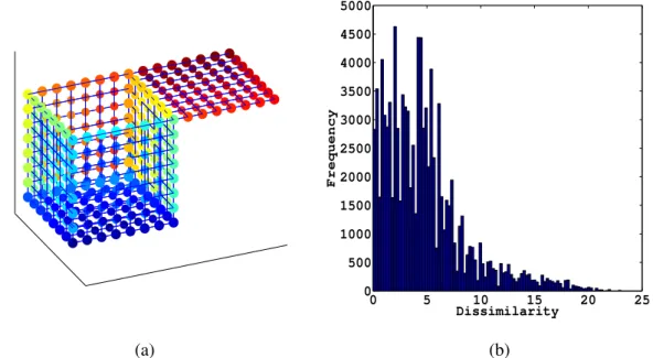
visualisation by all algorithms introduced in this chapter. The Open Box dataset [23] is a suitable benchmark, existing in 3-dimensional space with six 2-dimensional connected faces, one of which is an open lid. This is shown in figure 2.2a. The structure is

extensively analysed using variants of the nonlinear MDS in [24] and used to compare many different visualisation algorithms in [17]. The colouring of points represents the topological ordering of observations. The visualisations generated in this chapter should preserve the local neighbourhoods, keeping points from the base (dark blue), front face (cyan), sides (orange and light blue), connected side (yellow) and lid (red) in similar groupings. This benchmark serves as a comparison; however, it is an entirely artificial dataset and is therefore useful for visual comparison but not for drawing definitive conclusions as to which algorithm is ‘best’. The histogram of dissimilarities, where the dissimilarities between observations are the Euclidean distance, is shown in figure 2.2b. It is clear that the structure consists largely of local neighbourhoods withd_{i j}≤5. Larger dissimilarities exist because of the distance between the points on the lid at the far right of the plot and those in the bottom left corner of the front face.

Chapter 2 BACKGROUND (a) 0 5 10 15 20 25 0 500 1000 1500 2000 2500 3000 3500 4000 4500 5000 Dissimilarity Frequency (b)

Figure 2.2: 3-dimensional plot of the Open Box dataset. It is clear that the structure is composed of six 2-dimsensional planes with an open lid (red). The points here have been connected to their nearest neighbours to assist in checking how the visualisation algorithms distort neighbourhoods in the mapping process (left). The histogram of dis-similarities is also shown where the disdis-similarities are taken as the Euclidean distance between points (right).

2.2

Dissimilarity Mappings

2.2.1

The PCA/MDS Mapping

Principal Component Analysis (PCA) and Multi-Dimentional Scaling (MDS) are essentially different sides of the same coin as they both construct the same latent representations through slightly different methods. Firstly, PCA is introduced prior to explaining the process of MDS, following which the link between the two will be shown. PCA has been the standard method for visualising data across multiple fields for many years and is the starting point for many more robust visualisation algorithms shown in figure 2.1.

PCA can be derived from multiple perspectives, the two most popular being the minimal reconstruction error approach [6] or maximal preserved variance and decorrelation [25]. In this thesis the former is the more suitable so it will be introduced in that format. The minimal reconstruction error approach was derived by Pearson [6] where the dual

Chapter 2 BACKGROUND

relationship in the linear model is defined as:

RO→RP,xi→yi=WTxi, (2.1) RP→RO,yi→xi=Wyi. (2.2) W is an orthogonal matrix such thatWT =W†, whereW†is the Moore-Penrose

Pseudo-Inverse ofW. This ensures thatWTW =W†W =I_P. ThePsubscript here indicates the identity matrix is a square matrix of dimensionsP×P. The squared reconstruction error is given by:

EPCA=EX

kxi−WWTxik22

,

wherek.k2is the Euclidean distance. In the ideal case ofxigenerated by equation (2.2),

the mapping results in a reconstruction error of zero. This is becauseW will be full rank, ensuringWWT =I_OwhereI_Ois theO×Oidentity matrix. Unfortunately this is in almost all real situations not the case. In order to determineW, the above expectation can be expanded as follows:

E_PCA =E_X h xi−WWTxi T xi−WWTxi i , =E_XxT_i x_i−2xT_iWWTx_i+xT_iWWTWWTx_i , =EX xT_i xi−2xT_iWWTxi+xT_iWWTxi , =EX xT_i xi−xT_iWWTxi , =E_XxT_i xi −E_XxT_iWWTxi .

Splitting the error into these two parts allows for the optimumW to be found. The minimsisation ofEPCAis given by maximisingEX

xT_iWWTxi

, found whenWWT =IO.

Since data samples inX are finite, we can approximate this expression with the sample mean: E_XxT_iWWTxi ≈ _N1∑N_i xT_iWWTxi = _N1tr XTWWTX.

Here,X is the matrix set of observations,{xi}i=1:N, such that thei-th row ofX isxiwith

Chapter 2 BACKGROUND

orthonormal matrices (UTU =IN andVTV =IO) andΣmatrix with the diagonal

elements given by the singular values,E_PCA can be re-written as:

E_PCA=E_XxT_i xi

−E_XxT_i WWTxi

=tr XTX−tr XTWWTX.

Sincetr XTX=tr UΣTVTVΣUTfrom the singular value decomposition and using

the following two relations from [26, p. 6]:

• tr(ABC) =tr(CBA), • tr(XTX) =tr(ΣTΣ), it is clear that: E_PCA=tr UΣTVTVΣUT−tr UΣTVTWWTVΣUT, E_PCA=tr UTUΣTVTVΣ−tr UTUΣTVTWWTVΣ, E_PCA=tr ΣTΣ−tr ΣTVTWWTVΣ.

In the case whereP=O,EPCA is zero forW =V. Since the typical use of PCA is for

dimension reduction andP<Oan approximation must be used to makeW as linearly close toV as possible, namelyW =V I_O×P. HereI_O×P is a matrix made up of the firstP

columns of the identity matrixI_O. ThePdimensional latent variables are approximated by computing:

ˆ

yi_PCA=WTxi=IP×OVTxi. (2.3)

Classical multidimensional scaling (MDS) [18] will now be outlined as the other side of the coin to PCA. MDS seeks to preserve vector inner products from observations when generating visualisation points. Using a linear model, as with PCA, we denote the inner product matrixSby:

S =XTX,

= (WY)T(WY),

=YTWTWY,

Chapter 2 BACKGROUND

MDS has a particularly useful property thatX need not be a vectorial observation. Often observations are characterised by a pairwise dissimilarity matrix,D, of dimensions

N×N, where thei jth element,D_{i j}=d(i,j), is the pairwise dissimilarity between observationsiand j. FromD, the equivalent inner product matrixS, known as the Gram matrix, is found by double centering:

S=−1 2 D2− 1 ND 2₁ N1TN− 1 N1N1 T ND2+ 1 N21N1 T ND21N1TN , (2.4) whereD2is the element-wise square of the matrixD. This double centering removes the row and column means before adding back the total mean. In order to findY the

eigendecomposition ofSis performed: S =UΛUT, = (UΛ12)(_Λ12_UT), = (Λ 1 2UT)T(_Λ 1 2UT),

The optimal linear reconstruction (in a Least-Mean Square sense) ofY, ˆY, is then given by:

ˆ

YMDS=IP×NΛ

1

2_UT_{, (2.5)}

whereI_P×N is the firstPcolumns of theN×N identity matrixI_N. This ensures that only the requiredPdimensions are recovered by the MDS mapping algorithm. The

embeddings in equations (2.3) and (2.5) can be shown to be equivalent [17, p. 74-75]: ˆ Y_PCA =Yˆ_MDS, I_P×OVTX =I_P×NΛ 1 2UT, I_P×OVTVΣUT =IP×N(ΣTΣ) 1 2UT, I_P×OΣUT =IP×NΣUT.

The PCA/MDS embedding of the open box dataset is given in figure 2.3.

2.2.2

Locally Linear Embedding

MDS attempts to preserve global dissimilarities in visualisation spaces, however this can lead to a good overall mapping at the expense of good local reconstruction. Locally

Chapter 2 BACKGROUND

Figure 2.3: Open box embedded by PCA/MDS. The embedding is a poor representation of the original box as it is a top oriented squashed view. The top of the box remains separated from the other five sides, however the two open sides of the box have points overlapping which is not a true representation of their relative position in the observation space. This is because the linear relationship of equation (2.2) does not hold for the observed manifold,X.

Linear Embedding (LLE) [4] attempts to preserve dissimilarities in observation space by describing observations in terms of their local neighbours. This is done by imposing a locally Euclidean space on a manifold. The observed manifold is then characterised by a series of weighted neighbourhoods (either byk-nearest neighbours or anε-ball). The

visualisation space is constructed in a two step process.

The first step is to determine the weights associated with each neighbourhood, minimising the following error:

ELLE(W) = N

∑

∑

where_N(i)is the set containing all neighbours ofxi. This essentially sums all squared

distances between an observation and its locally linear reconstruction. Constraints are imposed onW such that:

• ∑jWi j=1,

Chapter 2 BACKGROUND

• Wi j =0∀ j∈/N(i).

The weights are determined by re-casting the error:

E_i=|xi−

∑

∑

∑

where{ηηηj,j=1, . . . ,k}are the set ofknearest neighbours of a pointi. The second part

comes from the first constraint above.C(i)_jl = (xi−ηηηj).(xi−ηηηl)is the local covariance

matrix. The weights corresponding to each observation ‘i’ denoted by the vector,wi, are

then given by:

W_{i j}= ∑lC(i) −1

jl

∑jlC(i)−1jl

, (2.7)

for j=1, . . . ,k, which are concatenated into the weight matrixW ={wi}i=1:N.

AlternativelyW can be found by solving the linear system:

∑

C(i)jlWil =1,

and rescaling so that∑jWj=1. It is proposed in [4] that ifCjl is singular or nearly

singular the following augmentation can be used, such that:

C_jl←C_jl+ ∆2tr(Cjl) K I,

where∆2is small compared to the trace ofCjl. This augmentation ensures that the

matrix can be inverted thanks to the ‘jitter’ term (right). This is a typical jitter

modification used to ensure numerically unstable matrices are invertible. Typical values of∆, for instance as used in [17], are 10−3. Alternatively a simpler jitter such as∆Ican

be added to ensure that the matrix is not singular in a less principled way.

The second step consists of embedding the points using their local reconstruction. This amounts to manipulating the visualised pointsy_ito minimise the error with respect to the set of latent points,Y:

ELLE(Y) = N

∑

∑

Chapter 2 BACKGROUND

whereW is given from equation (2.7). Two constraints are imposed uponY:

• ∑iyi=0⇒centred around the origin

• C_YY = _N1YYT =I⇒unit covariance soE_LLE(Y)cannot be minimised by arbitrary rotations or rescalings.

The embedding is found by the well-posed eigenvalue problem:

ELLE(Y) =

∑

∑

∑

∑

∑

using the same properties as above. The entries ofMare given by:

M= (I−W)T(I−W),

which is sparse (since the elements ofW are non-zero only for thekneighbours of each pointi), symmetric and positive definite. The co-ordinates ofY are found by computing the bottomP+1 eigenvectors ofM(wherePis the visualisation dimension, e.g. 2) and discarding the bottom eigenvector as its eigenvalue is 0 (since∑iyi=0):

YLLE =Uˆ,

where ˆU is the bottomN−1 :N−Peigenvectors. This ensures that the best linear reconstruction of the neighbourhoods ofX are given byY.

The Open Box visualisation using LLE with four neighbours (the same as that of [17]) is shown in figure (2.4). In contrast to the PCA mapping, the sides of the box (light blue and orange) are no longer flattened. The six surfaces of the box are all well reconstructed in themselves, appearing as parallelograms. On the other hand, the relative distances of the sides with respect to the bottom of the box (dark blue) are not well preserved. This is clear from the overlap of points in visualisation space which are not close in observation space, for instance the front face which overlaps the bottom face. The good local

reconstruction comes at the cost of the global distribution of points caused by the LLE error function.

Chapter 2 BACKGROUND

Figure 2.4: Open box embedded by LLE. The six surfaces of the box are all well recon-structed in themselves, appearing as rectangles. The relative distances of the sides (light blue and orange) with respect to the bottom of the box (dark blue) are not well preserved.

2.2.3

Sammon Mapping & NeuroScale

This section will outline the Sammon Mapping process for visualisation before describing the NeuroScale mapping.

Sammon map

Taking a more global approach to visualisation, the Sammon map [9] attempts to construct a set of visualisation points,Y, by preserving relative dissimilarities. This is done by matching the dissimilarity matrices, as opposed to inner product matrices as MDS does. This constructs more reliable visualisations, as shown in [17]. Denoting the dissimilarities between observationsdx(i,j)and between visualised pointsdy(i,j)the

error to be minimised is:

E_Sammon= 1 c N

∑

where the normalisation constantc=∑N_i,i<jdx(i,j). This function is commonly known

as the Standardised Residual Sum of Squares (STRESS) measure. It is important to note that no assumption is made aboutdx(i,j)and so can be application-specific (e.g. [27] or

Chapter 2 BACKGROUND

Figure 2.5: Open box embedded by Sammon mapping. The sides of the box are still attached to the top and bottom faces, but are correctly placed directly on top. The front face of the box opposite the open lid is squashed in a similar way to that of PCA/MDS and the bottom corners appear torn.

usually taken to be the Euclidean distance;d_y(i,j) =ky_i−y_jk₂. Originally Sammon proposed an iterative quasi-Newton style update rule such that:

y_i←y_i−α ∂ESammon/∂yi |∂2ESammon/∂y2_i|

,

whereαis a learning rate. In reality this can result in quickly finding poor local minima

so other gradient-based optimisation procedure can produce more reliable visualisation spaces. PCA or MDS can be used as an initialisation ofY, but this can provide minima close to, but not as optimal as, the global minima. The derivative of (2.9) is given by:

∂ESammon ∂y_i = −2 c

∑

wherecis again given byc=∑Ni,i<jdx(i,j). The use of Quasi-Newton optimisation is

not essential here, other gradient-based optimisers could be used e.g. Scaled Conjugate Gradients (SCG). Unlike MDS, PCA and LLE, Sammon Maps embed in a nonlinear way.

The 2-dimensional embedding of the Open Box dataset using Sammon mapping is shown in figure 2.5. The mapping is optimised using Quasi-Newton gradient descent

Chapter 2 BACKGROUND

with random initialisation to avoid the potential PCA-initialisation sink. The nonlinear embedding process allows for curvature to be imposed on the manifold, by not placing a linear mapping on the observation space. This causes the sides of the box to still be attached to the top and bottom faces, without being placed directly on top. The front face of the box opposite the open lid is squashed in a similar way to that of PCA/MDS and the bottom corners appear torn. Despite these inaccuracies the overall shape of the manifold can be easily recognised from the visualisation.

In [29] an extension to the Sammon map using feed forward Radial Basis Function (RBF) networks was outlined which will be described in the next section. An introduction to RBF networks is given in appedix A.

NeuroScale

The extension of the Sammon map using RBF’s is called NeuroScale (NS). Variants using a Multi-Layer Perceptron network were also proposed in [30]. As already mentioned, the STRESS function, in contrast to the standard learning procedure of RBFs, requires nonlinear optimisation. Learning weights through gradient descent is the standard approach in the training of Artificial Neural Networks. However, a more robust and efficient method for training the NS RBF network was described in [31]. True observation targets,T, do not exist but the ‘Shadow Targets’ algorithm involves generating a series of synthetic targets,ti:

ti=yi−α ∂ESammon ∂y_i , ˆ W =Φ†T, ˆ Y =ΦWˆ,

with ∂ESammon

∂yi given by equation (2.2.3). This iterative steepest descents process is

repeated until convergence usingαas a learning rate. The NS algorithm works best

whenΦis as representative as possible of the data, i.e. when the number of centres is as

Chapter 2 BACKGROUND

parameterised machine learning tasks, NS cannot overtrain [29], [32]; performing implicit auto-regularisation due to the network centres and curvature with respect to the STRESS function. In addition to this, the RBF network is infinitely smooth meaning out of sample observations will also be topographically mapped. With this in mind a suitably interpolated data space in NS would generate an identical Open Box visualisation to that of the Sammon mapping and is therefore not included here. The Shadow Targets

algorithm is used extensively in chapters 3 and 7 in this thesis as an optimisation procedure.

Standard NS was extended in [33] to account for uncertainty using isotropic Gaussians to describe observations and mapped points. This method will be discussed in chapter 3.

2.3

Graph Distance Mappings

Graph distance mappings take a slightly different approach to visualisation than dissimilarity-based mappings. They treat observations as objects of a graph to be

represented in a visualisation space. Two methods are outlined; Isomap, relying on graph distances, and Laplacian Eigenmaps (LE) using the graph Laplacian for optimisation.

2.3.1

IsoMap

The Isomap algorithm [5] uses neighbourhood structures like LLE,k-neighbourhoods or

ε-balls, to construct a graph characterising observations. Graph edges are labelled with

Euclidean lengths, giving a sparse weighted graph (note that other dissimilarity measures can be used, though this is not common in the literature). The remaining graph distances between observations are computed in a pairwise manner using geodesic distances computed by Djikstra’s [34] or Floyd’s [35] algorithms and stored as a dissimilarity matrix,D(many implementations such as that in [20] use Djikstra’s algorithm as default). This dissimilarity matrix is treated as an alternative to dissimilarities in MDS, but the embedding procedure is then identical for Isomap as for MDS.

The dissimilarity matrixDis converted into an inner product (Gram) matrix,S, by double centering (equation 2.4). As with MDS the eigendecomposition ofSgives

Chapter 2 BACKGROUND

S=UΛUT with eigenvectorsU and eigenvalues as diagonal elements ofΛ. The

P-dimensional embedding of the observationsX, given byD, is:

Y =I_P×NΛ

1

2_UT, _(2.11)

This embedding attempts to minimise the standard MDS error:

E_Iso=

∑

kd_x(i,j)−d_y(i,j)k2, (2.12) by inner product eigendecomposition. Isomap is an efficient and popular tool for

creating representative visualisations of complex data. Geodesic distances are a much more realistic dissimilarity between points on a manifold than the assumption that a manifold is Euclidean, for example in Riemannian manifolds [36]. This fact is reinforced by the work in Machine Learning on Riemannian Manifolds (for instance [36], [15]). There are three particular weaknesses worth noting with Isomap:

1. The sensitivity of the map to choice ofkorε,

2. The calculation of dissimilarities in the presence of noise or uncertainty. 3. The linear embedding formed by MDS.

These can cause short-circuits in the graph construction leading to an incorrect over- or underestimation of the distance between observations. An important note is thatkorε

should be chosen such that the graph is fully connected (no geodesic distances should be infinite). The embedding generated is a linear mapping and is therefore unable to

appropriately characterise a highly nonlinear mapping function. An alternative method using geodesic dissimilarities was proposed in [37],[38]. These dissimilarities were combined with the Sammon map, relying on the benefits of the two methods, called the Geodesic Nonlinear Map (GNLM) . The training procedure for GNLM is the same as that of the Sammon map but withd_x(i,j)given by geodesic distances and graph neighbourhoods.

Chapter 2 BACKGROUND

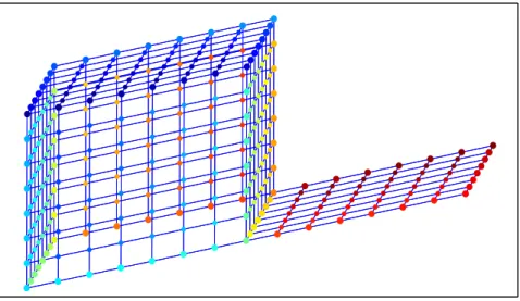
Figure 2.6: Open box embedded by Isomap using four neighbours. The front face of the box has been overlapped with the bottom of the shape and the mapping has imposed a curved surface on the box lid which is in fact rectangular in the original space. The box sides are squashed and therefore not representative of the original structure.

k=4 neighbours and the overall box structure is clear. This seems an improvement on the LLE box, but there are still squashed sides similar to those of the PCA/MDS box. The front face of the box has been overlapped with the bottom of the shape and the mapping has imposed a curved surface on the box lid which is in fact rectangular in the original space. If the neighbourhood structure is extended to incorporatek=8

neighbours, a more visually satisfactory image is achieved in figure 2.7. Here the lid is made approximately rectangular and there is less overlapping in the box sides due to the curvature imposed here. The distances from the box front to the bottom are more

faithfully preserved with less overlapping. This does highlight a main issue with neighbourhood based mappings, namely that the change in visualisation spaces can be significant with changes inkorε. It is noteworthy that the visualisation space remains

largely unchanged for increases in neighbourhood size beyond eight neighbours. The only differences are seen in the lid and bottom becoming more rectangular, as in the MDS mapping of figure 2.3.

Chapter 2 BACKGROUND

Figure 2.7: Open box embedded by Isomap with eight neighbours. The lid is made ap-proximately rectangular and there is less overlapping in the box sides than the k =4 mapping thanks to the curvature imposed here. The distances from the box front to the bottom are also more faithfully preserved with less overlapping.

2.3.2

Laplacian Eigenmaps

Laplacian Eigenmaps [19] is another graph-based embedding process with connections to LLE. The algorithm begins with a dissimilarity matrix,D, constructed by pairwise dissimilarities between observations. Following this step, akorε-ball neighbourhood is

found. These neighbourhoods are used to build a graph with corresponding adjacency matrixA(an (i,j) binary matrix with elements 1 when observations (i,j) are adjacent, or neighbours, and 0 otherwise). The graph weight matrixW is then calculated by use of the ‘heat kernel’ (this is typically known as a Gaussian function in other areas of the literature, but is referred to here as the ‘heat kernel’ as it is in [19]):

W_{i j}=A_{i j}exp −kxi−xjk22 2T2 , (2.13) whereT is the temperature parameter. T is a user-specified parameter in the interval

[1,∞)with popular choices being 1 or∞. The dissimilarity measure does not necessarily

need to be Euclidean and can be replaced with other measures capable of dealing with uncertainty as will be shown in section 3. A simpler weight function, often used in the literature is whereT tends to infinity such thatW =A. These weights are then used to

Chapter 2 BACKGROUND

compute the graph Laplacian [39]:

L=W−G,

whereGis a diagonal matrix with entriesGii=∑Nj=1Wi j. In order to preserve the range

of eigenvalues to create a standard embedding framework, and therefore a standard co-ordinate range, the Laplacian is then normalised:

L0=G−12_LG− 1 2.

This ensures the eigenvalues are within the range 0≤λ≤2 [40]. Two Laplacians for

entirely different graphs can then be compared without the issue of rescaling; only co-ordinate rotations need to be considered. The embedding error to be minimised is:

ELE= 1 2 N

∑

subject toY GYT =I_P×P, ensuring that the error cannot be minimised by the arbitrary rescaling ofY. This error can be minimised by computing the eigendecomposition of

L0=UΛUT. The embedded co-ordinates are found by taking the smallestP+1

eigenvectors and discarding the smallest eigenvector (since the above constraint forces the eigenvalue to be 0). This is because the error function in equation (2.14) can be re-written as ‘tr(Y L0Y)’, the solution of which is given by the same eigen-formulation. The remaining eigenvectors, ˆU (of dimensionsP×N) give the embedding as:

Y =U Gˆ 12_.

Figure 2.8 shows the embedded Open Box computed by LE. The graph was constructed with four neighbours (creating a fully connected graph) as with Isomap and LLE; however, here the visualisation space remains largely unchanged with increasingk. The temperature parameter used here is set to unity, as is common in the literature, but tests were also run with increasingT (values uniformly sampled in the range(1,106)),

Chapter 2 BACKGROUND

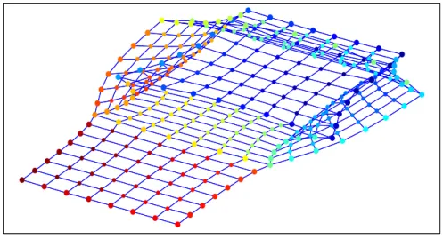
Figure 2.8: Open box embedded by Laplacian Eigenmapping with four neighbours. The algorithm has successfully unfolded the box from the open section. The box lid on the right hand side is separated from the bottom and front face. The front surface undergoes a level of squashing which is unrepresentative of the observations and the other two open sides to a lesser degree as well. The global and neighbourhood structure has however been preserved faithfully.

resulting in no change in the visualised coordinates. This is likely due to the relatively small and identical Euclidean distances between local points in the observation space, ensuringT in the heat kernel plays a relatively insignificant role. The artificial curvature imposed here appears on first inspection to have distorted the mapping. However, the algorithm has successfully unfolded the box from the open section. The box lid on the right hand side is separated from the bottom and front face. The front surface undergoes a level of squashing which is unrepresentative of the observations and the other two open sides to a lesser degree as well. The global and neighbourhood structures have however been preserved faithfully.

2.4

Latent Variable Models

The approach for generating visualisation spaces in Latent Variable Models (LVMs) is altogether different to that of dissimilarity preservation and graph-based mappings. LVMs assume a generative process in which observations are treated as the functional output and the latent points, (representing the visualisation space) which most likely

Chapter 2 BACKGROUND

generated those observations, are found. In this sense PCA is also a LVM. LVMs therefore seek to learn the inverse function to dissimilarity preservation mappings. As such there are rigid assumptions with each method. There will be a change in notation from the previous sections; denoting observations byY and latent points byX such that

Y = f(X), consistent with that of the literature (e.g. [7],[2],[8]). Two LVMs are

discussed below; the Generative Topographic Mapping and the Gaussian Process Latent Variable Model. A currently popular LVM called the Deep Gaussian Process [13] is described in Appendix B and not here as it is not topographic.

2.4.1

Generative Topographic Mapping

The probabilistic extension of Kohonen’s Self Organising Map [41] is known as the Generative Topographic Map (GTM) [7]. It is a generative model assuming data observations are created by a latent grid, often assumed rectangular.

The distribution of observations, p(y_i|x,W,β)are spherical Gaussian kernels,

N

parameterised mean function with weightsW,m(x,W). The distribution is therefore:

p(y_i|x,W,β) = β 2π l₂ exp −β 2kyi−m(x,W)k 2 , (2.15) wherel is the dimensionality of the observations. The prior distribution over the latent grid, p(x), is given by:

p(x) = 1 c c

∑

p(x|y_i,W,β) = p(yi|x,W,β)p(x)

Chapter 2 BACKGROUND

In order to compute this posterior, the marginal likelihood must be calculated:

p(y_i|W,β) =

Z

p(y_i|x,W,β)p(x)dx.

This integral is typically analytically intractable for many prior choices but since the prior is a grid of delta points, the marginal likelihood becomes:

p(y_i|W,β) = 1 c c

∑

The data log-likelihood is given by:

L

N

∑

log(p(y_i|W,β)).

The mean function,m(x,W), in equation (2.15) is typically taken to be an RBF network as described in appendix A. Other extensions using Gaussian Processes (GPs) and mean field approximations for the marginal likelihood have also been proposed [42]. Using an RBF network in this framework allows for an Expectation-Maximisation (EM)

optimisation procedure outlined in Appendix C.

Visualisation

In order to generate the visualisation space, summary statistics of the posterior must be used. The mean can be approximated by:

ˆ xi= c

∑

∑

The posterior can be multimodal, which is revealed by a comparison of the mean and mode of the distribution, where the mode is given by:

ˆ xi=arg max g(r) p(g(r)|y_i) =arg max g(r) Pir(Wopt,βopt).

Chapter 2 BACKGROUND

Figure 2.9: Open box embedded by GTM. The global structure has been unfolded from the open top, but the box front (cyan) and lid (red) are clearly squashed. It is clear that the mapping has torn the corners of the box open leading to a separation of naturally close observation points but the box floor (dark blue) and side connecting the floor to the lid (yellow) are faithfully represented.

Large discrepencies between means and modes of latent visualised points will indicate that a less reliable distribution has been created.

The GTM visualisation of the Open Box dataset is shown in figure 2.9 using a 10×10 latent grid and a 4×4 grid of basis functions with mean points shown, following the mapping procedure of [17]. The global structure has been unfolded from the open top, but the box front (cyan) and top (red) are clearly squashed. It is clear that the mapping has torn the corners of the box open, leading to a separation of naturally close

observation points. On the other hand the box floor and side connecting the floor to the lid are faithfully represented. The posterior distribution is multimodal, causing many of the modal points to be separated from the mean. Many of the mode points sit atop each other which reinforces the notion that clusters in observation space are not ideally represented. The analysis was repeated with larger latent grids (20×20 and 30×30) where the transition between faces becomes smoother, but the tears appear in the same regions. Even with these larger latent grids the distribution is still multimodal.

Finally, the magnification factors [43] of the latent grid mapping are superimposed into the visualisation, showing which areas of the observation space have been magnified or

Chapter 2 BACKGROUND

Figure 2.10: Open box embedded by GTM with points superimposed upon the mag-nification factors. These magmag-nification factors indicate that the areas well preserved in visualisation space (the box bottom and connecting side) have been magnified more than the corners and lid indicating the trustworthiness of the mapping.

shrunk to accomodate the data. These magnification factors indicate that the areas well preserved in visualisation space (the box bottom and connecting side) have been

magnified more than the corners and lid indicating the trustworthiness of the mapping in these regions.

GTM offers an interesting alternative to data visualisation when compared with the methods described above but there are certain drawbacks:

• The noise model of isotropic Gaussians is not a realistic situation due to the geometry of Gaussians in high dimensions. This will be more thoroughly explained in chapter 3.

• The rectangular grid is an unrealistic latent space and is limited to a 1 or 2-dimensional visualisation.

• The number of kernels for interpolation of data is limited to be at maximum the size of the latent grid. This ensures the learning phase is quick and not relatively complex or highly parameterised whereas the ideal situation would allowN

kernels such as in NS.

Chapter 2 BACKGROUND

visualisation. In order to assume a generative model, restrictions must be placed upon the observations, latent space and mapping functions. These restrictions can often be too restrictive for real world observations. In order to preserve observations in a topographic way, the latent grid should be as large as is possible whilst keeping the number of basis functions low, to avoid overfitting in the regression framework (m(x,W)). This should circumvent the short circuiting in the training phase where two points close in

observation space sit directly atop of one another in latent space.

2.4.2

Gaussian Process Latent Variable Model

The Gaussian Process Latent Vatiable Model (GPLVM) is a probabilistic model using a latent space similar to that of GTM. The two main differences between GTM and GPLVM are:

1. The mapping function from latent to observation space is restricted to a Gaussian Process (GP).

2. The latent space is no longer restricted to a lattice of delta functions.

A short introduction to GPs in the context of the GPLVM will now be given; a thorough introduction is given in [2] and [44]. For observationsY ∈_RM_:y

i= f(xi) +εi. GP

outputs are scalar by nature, but some methods for extending to ‘multiple output GPs’ (vector outputs) exist (for example [45],[46] and [13]). The GP used by the GPLVM uses a much simpler notion to create vector outputs, demanding that output dimensions are independent using separate mapping functions:ym_i = f_m(xi) +εmi . In the GP formulation p(εi) =

N

N

mean in general and can be written as:

p(Y|X) = M

∏

∏

N

K

wherey_mis a column vector containing theN entries fromY for dimensionm.

K

Chapter 2 BACKGROUND

exponential (SE), or Gaussian, kernel:

K

diagonal weight matrix. The ARD matrix learns the dimensions ofX which are

significant in the mapping process. In the standard regression case whereX is observed as well asY, the parameters are learned using gradient descent in a maximum likelihood (ML) fashion from the likelihood equation (2.17). In the GPLVM caseX must be learned as well as the kernel hyperparameters, for which there are two main methods:

1. [8] Iterative optimisation of the kernel hyperparamters based on the ML approach for the currentX, then optimising p(y|x,σ2_f,W,β)with respect toX.

2. [47] In a fully Bayesian framework a variational lower bound is used to optimise the marginal likelihood p(Y) =R

p(Y|X)p(X)dX. This integral is in general analytically intractable due to the nonlinear interactions in the kernel functions. The automatic training of the ARD parameters inW allows for the dimension ofX to be larger than two and only the two most relevant dimensions visualised. As with RBFs, GPs with SE kernels are infinitely smooth but are not topographic without imposing a ‘back constraint’. This back constraint involves the addition of the Sammon STRESS error function from equation (2.9) to the GP likelihood with a multilayer perceptron (MLP) network used to minimise this error [48]. A formal definition of MLP networks is given in chapter 7, all that is important to note here is that it optimises over the STRESS function with respect to the latent pointsY and the observations,X. The use of the MLP and imposition of the STRESS measure ensures that the latent points learned are

topographic.

Figure 2.11 shows the GPLVM visualisation of the open box using back constraints to ensure the mapping learned is topographic. The algorithm unfolds the structure from the open top and curves all sides to preserve the topological ordering. The points from the box floor remain relatively uniform in the mapping which is an improvement on the

Chapter 2 BACKGROUND

Figure 2.11: Open box embedded by GPLVM with back constraints. It is clear that the algorithm has unfolded the structure from the open top and curves all sides to preserve the topological ordering. The points from the box floor remain relatively uniform in the mapping. The points from the lid appear to have been squashed into a relatively small area, in the top-left of the latent space, compared to that of the sides and bottom, but are still correctly ordered and their relative distance within the lid points is preserved. The box front (cyan) is not well mapped with the vertical dimension of points almost placed directly atop of one another and the entire front face is placed unusually far from the rest of the box.

GTM mapping. The points from the lid appear to have been squashed into a relatively small area, in the top-left of the latent space, compared to that of the sides and bottom, but are still correctly ordered and their relative distance within the lid points is preserved. Each row of points which make up the front face is removed from their local

neighbourhours on the other faces of the box. The box front is not well mapped with the vertical dimension of points almost placed directly atop of one another and the entire front face is placed unusually far from the rest of the box. The GPLVM also allows for computation of the posterior probabilityP(X|Y)which can be superimposed into the visualisation of the box, as shown in figure 2.12. The areas of higher posterior probability are shown in pink; with blue denoting low probabilities. This probability map indicates that the GPLVM has not faithfully interpolated the data space as there are regions of apparent high probability which contain either a low density, or no points. The box lid has the opposite problem of significantly high density of points with a low

Chapter 2 BACKGROUND

Figure 2.12: Open box embedded by GPLVM with back constraints with posterior prob-ability surface shown. The areas of higher posterior probprob-ability are shown in red with blue denoting low probability. This probability map indicates that the GPLVM has not faithfully interpolated the data space as there are regions of apparent high probability which contain either a low density or no points. The box lid has the opposite problem of significantly high density of points with a low posterior probability of observation. uniformly generated with the same number of points as the other sides.

Compared to GTM this approach is more robust, but it still suffers from restrictions of independence between dimensions ofY and between latent pointsX. The assumption that all observations,Y, are normally distributed is typically taken to be realistic. The extent to which this is true depends on the application. The concept of the visualisation of posterior probabilities is useful for judging expected location of visualised datapoints. However, even in this simple case of a 3-dimensional embedding the probability surface has been incorrect and misleading. An interesting note about the back constraints imposed here is that the distance measures used ford_xandd_yhave not been explicitly specified. The Euclidean distance used in the algorithm in [22] can be deemed

appropriate for the latent variablesX as the priors overX are isotropic, unit covariance Gaussians. For this case of distribution many dissimilarity measures incorporating uncertainty reduce to the Euclidean distance. On the other hand, the observationsY are learned with specific covariance measures - the main benefit between Gaussian

Processes over other Machine Learning tools. Therefore, taking the Euclidean distance asd_y wastes this additional learned information. Other methods for visualisation

Chapter 2 BACKGROUND

incorporating uncertainties such as probabilistic NeuroScale (outlined in Chapter 3) allow for user-specified dissimilarity measures.

2.5

Quality Criterion

The mappings discussed in this chapter all work in different ways and optimise separate objective functions. To this end, it is difficult to assess how well one algorithm performs in generating a visualisation compared to another, particularly since it is easy for

visualisations to appear to have structure when there is none [49]. The different open box embeddings show this; some researchers favour the Isomap embedding over the Sammon map. This section will outline some quality criteria which can offer a comparison

between mappings based on data ranking. For a more thorough guide see [24].

2.5.1

Rank

The notion of rank,R(i,j), is outlined in [50]. R(i,j)is defined as the number of observations closer toithan jis. Formally this is:

R_data(i,j) = n k:DO_ik<DO_{i j} o ∪nk:DO_ik=DO_{i j},k< j o , (2.19)

whereU is the union between sets,|.|denotes set cardinality andDO_{i j} is the dissimilarity between observationsiand j. The rank of pointsiand jin the latent visualisation space is:

R_Latent(i,j) =

k:DL_ik<DL_{i j} ∪

k:DL_ik=DL_{i j},k< j , (2.20)

whereDL_{i j} is the dissimilarity between latent visualised points. Note that

R_data(i,i) =R_latent(i,i) =0 andR_data(i,j)6=R_latent(i,k)even whenD_ik=Di j but j6=k.

2.5.2

Trustworthiness and Continuity

Two important ways to characterise whether a visualisation is topographic were

Chapter 2 BACKGROUND

become close in observation space, impairing the trustworthiness (T) of the embedding. The opposite case being where similar observations are made dissimilar in visualisation space, causing a loss in continuity (C).

Using_Nk_data(i)and_Nk_latent(i)to define the set of theknearest neighbours of pointsiin data and latent spaces respectively. In order to define both T and C, neighbourhood intruders and leavers must first be defined. Intrudersk(i) is the set of points in the k-neighbourhood of observation(i)in latent space but not in the original observation space:

Intrudersk(i) =Nklatent(i)\Nkdata(i),

where ’\’ represents the intersection of the relative complement of the set. Consequently the Leaversk(i)are the set of observations in thek-neighbourhood of (observation)iin

the observation space but not in the latent space:

Leavers_k(i) =_Nk_data(i)\_Nk_latent(i).

Trustworthiness can now be defined as:

T(k) =1− 2 ΓTC N

∑

∑

C(k) =1− 2 ΓTC N

∑

∑

Chapter 2 BACKGROUND

quality measure described in [24] as:

Q_TC(k) =2 T(k)C(k)

T(k) +C(k). (2.24)

As with the individual T and C measures, a higher value ofQTC indicates a better

mapping.

2.5.3

Mean Relative Rank Error

Working similarly to the T and C measures, mean relative rank error (MRRE) [17] compares the ranks of the observation and visualisation spaces:

MRRE_data(k) = 1 ΓMRRE N

∑

∑

which corresponds to trustworthiness. On the other hand, continuity relates to

MRRE_latent: MRRElatent(k) = 1 ΓMRRE N

∑

∑

∑

Better visualisation quality is indicated by lower values of MRRE. The values are zero whenR_latent(i,j) =R_data(i,j). MRRE weights rank error, unlike T and C. As withQTC

the two MRRE measures are combined in [24]:

Q_MRRE(k) =2 (1−MRREdata)(1−MRRElatent)

(1−MRRE_data) + (1−MRRE_latent). (2.27)

Chapter 2 BACKGROUND

2.5.4

Local Continuity Meta-Criterion

The continuity measure,C, looks at global continuity, whereas the local continuity meta-criterion (LCMC) [52] measure is interested in strict neighbourhoods:

LCMC(k) = 1 Nk N

∑

2.5.5

Quality of Open Box embeddings

In this thesisQ_TC,QMRRE andLCMCfrom equations (2.24), (2.27) and (2.28) will be

used to quantitatively assess the performance of the visual