A Many-Objective Evolutionary Algorithm Using A
One-by-One Selection Strategy
Yiping Liu, Dunwei Gong, Jing Sun, and Yaochu Jin,
Fellow, IEEE
Abstract—Most existing multi-objective evolutionary algo-rithms experience difficulties in solving many-objective optimiza-tion problems due to their incapability to balance convergence and diversity in the high-dimensional objective space. In this paper, we propose a novel many-objective evolutionary algorithm using a one-by-one selection strategy. The main idea is that in the environmental selection, offspring individuals are selected one by one based on a computationally efficient convergence indicator to increase the selection pressure towards the Pareto optimal front. In the one-by-one selection, once an individual is selected, its neighbors are de-emphasized using a niche technique to guarantee the diversity of the population, in which the similarity between individuals is evaluated by means of a distribution indicator. In addition, different methods for calculating the con-vergence indicator are examined and an angle-based similarity measure is adopted for effective evaluations of the distribution of solutions in the high-dimensional objective space. Moreover, corner solutions are utilized to enhance the spread of the solutions and to deal with scaled optimization problems. The proposed algorithm is empirically compared with eight state-of-the-art many-objective evolutionary algorithms on 90 instances of 16 benchmark problems. The comparative results demonstrate that the overall performance of the proposed algorithm is superior to the compared algorithms on the optimization problems studied in this work.
Index Terms—Many-objective optimization, evolutionary multi-objective optimization, performance indicator, cosine sim-ilarity, convergence, diversity.
I. INTRODUCTION
M
ULTI-objective optimization problems (MOPs) are commonly seen in real world applications, e.g., in-dustrial scheduling [1], controller design [2], [3], environ-mental/economic dispatch [4], and many others. MOPs are characterized with multiple conflicting objectives, indicating that there is no single optimal solution to these problems, rather a set of trade-off solutions, known as the Pareto optimal set. In the literature, MOPs with more than three objectives are often referred to as many-objective optimization problems (MaOPs) [5]–[9].Y. Liu is with School of Information and Electrical Engineering, Chi-na University of Mining and Technology, Xuzhou 221116, ChiChi-na. e-mail: [email protected]
D. Gong is with School of Information and Electrical Engineering, China University of Mining and Technology, Xuzhou 221116, China, and School of Electrical Engineering and Information Engineering, LanZhou University of Technology, Lanzhou 730050, China. e-mail: [email protected]
J. Sun is with School of Science, Huai Hai Institute of Technology, Lianyungang 222005, China. e-mail: [email protected]
Y. Jin is with the Department of Computer Science, Universi-ty of Surrey, Guildford, Surrey, GU2 7XH, United Kingdom. e-mail: [email protected]
Manuscript received 2015; revised 2015.
Over the past two decades, a large number of multi-objective evolutionary algorithms (MOEAs) have been proposed. Gen-erally speaking, the selection strategy plays a key role in most MOEAs, which needs to take both the convergence of the solutions to the Pareto optimal front and the distribution of the solutions into account.
Pareto-dominance-based MOEAs, e.g., nondominated sort-ing genetic algorithm II (NSGA-II) [10] and strength Pareto evolutionary algorithm 2 (SPEA2) [11], are the most popular among various methods. These algorithms employ the Pareto dominance as the primary selection criterion, where non-dominated solutions are always preferred for good conver-gence. To promote a good distribution of the solutions, a diversity related secondary selection criterion is adopted as well. Dominance-based MOEAs have been proved successful in solving a large number of MOPs. However, their perfor-mance will seriously deteriorate in solving MaOPs. One main reason is that the proportion of non-dominated solutions in the population considerably rises as the number of objectives increases [12], leaving the dominance-based selection criterion unable to distinguish solutions. As a result, the diversity based criterion will play a crucial role in selection, leading to solutions far away from the Pareto optimal front being maintained [13].
An effective approach to improving the ability of dominance-based MOEAs to solve MaOPs is to redefine the dominance relationship. A large body of research along this line has been reported, e.g., dominance area control [14], L-optimality [15], fuzzy Pareto dominance [16], etc. Although these modified dominance relationships have been shown to be able to improve the convergence of MOEAs for solving MaOPs, they may also cause the population to converge to a sub-region of the Pareto optimal front [17].
An alternative way to enhance the ability of dominance-based MOEAs for MaOPs is either to improve the diversity-based secondary selection criterion, or to replace it with other selection criteria. For instance, a diversity management operator is employed to adjust the requirement on diversity in mating and environmental selection [18]. By shifting the position of a solution in sparse regions, a shift-based density estimation (SDE) was proposed to discard solutions that lead to poor convergence [19]. An extension of NSGA-II for solving MaOPs, termed NSGA-III was developed in [20], which uses a reference-point-based secondary criterion for maintaining diversity. In [21], following the idea of preferring the knee points among non-dominated solutions, a knee point driven evolutionary algorithm (KnEA) was proposed for many-objective optimization.
Unlike dominance-based MOEAs, decomposition-based MOEAs have been found to be very promising for many-objective optimization. One typical example of this class of algorithms are MOEA/D [22] and its variants [23]–[27]. In MOEA/D, the diversity of a population is maintained by a set of predefined well distributed reference vectors. Based on these reference vectors, the objectives of an MOP are aggre-gated into a number of scalarizing functions, each of which generating a single scalar value. Individuals in a population are guided to search towards the Pareto optimal front in the directions specified by the reference vectors by minimizing these scalarizing functions. MOEA/D has been demonstrated efficient in solving both MOPs and MaOPs. However, one known problem of MOEA/D is that uniformly distributed reference vectors do not necessarily lead to uniformly dis-tributed solutions, particularly for problems with irregular (i.e., nonuniform) Pareto optimal fronts.
Grid-based algorithms, e.g.,ε-MOEA [28], GrEA [29], and MaOPSO/2s-pccs [30], are also very competitive MOEAs for solving MaOPs. Grids are very effective for measuring the distribution of solutions according to their positions. In these algorithms, the objective space is first divided into a grid of hypercubes. Then, some convergence-related selection criteria, e.g., the dominance relationship of the hypercubes and the distance between a solution and the origin of its hypercube, are utilized so that each non-dominated hypercube contains no more than one solution. However, the adaptation of the grid size for different optimization problems is non-trivial.
Different from the above methods, indicator-based evolu-tionary algorithms (IBEAs) [31] adopt a single indicator which accounts for both convergence and distribution performances of a solution set. Therefore, solutions can be selected one by one based on their influence on the performance indica-tor. Among others, hypervolume is a widely used indicator in IBEAs. Unfortunately, the computational complexity for calculating hypervolume increases exponentially as the num-ber of objectives increases, which makes it computationally prohibitive for MaOPs. To address this issue, HypE [32] uses Monte Carlo simulations to estimate the hypervolume, where the accuracy of the estimated hypervolume can be trade off against the available computational resources. Recently, R2 [33] and the additive approximation [34] were also proposed to further enhance the computational efficiency of IBEAs for solving MaOPs.
The effectiveness of IBEAs for solving MaOPs lies in the fact that performance indicators such as hypervolume can account for both convergence and distribution of the solution set. Intuitively, it is also likely to consider convergence and distribution of a solution set separately, e.g., by simultaneously measuring the distance of the solutions to the Pareto optimal front, and maintaining a sufficient distance between each other. Motivated by this idea, we propose here a many-objective evolutionary algorithm using a one-by-one selection strategy, 1by1EA for short. In 1by1EA, solutions are selected according to a convergence indicator and a distribution indicator. The former measures the distance between a solution and the Pareto optimal front, while the latter measures its distance to each other. In each step of the selection procedure, only
one solution with the best value of the convergence indicator is selected. Then, based on the distribution indicator, the solutions close to the selected one are de-emphasized using a niche technique. Thus, superior solutions are selected one by one and the needed calculation in each generation is little. On the contrary, calculating the indicator in IBEAs is computationally expensive, not only because the calculation involves both convergence and distribution, but also because it has to be recalculated once a new solution is selected.
The main contributions of this work can be summarized as follows:
(1) A general evolutionary framework, termed 1by1EA is p-resented, where solutions in the current population are selected one by one based on a convergence indicator. The neighboring solutions of the selected solution are de-emphasized using a niche technique, in which their similarities are evaluated by a distribution indicator. One benefit of this selection strategy is that it is able to easily balance the need for convergence towards the Pareto optimal front and the requirement on diversity of the population.
(2) A distribution indicator based on the cosine similarity is proposed for effectively evaluating the distance between solutions in the high-dimensional objective space. Compared with the distribution indicator based on the Euclidean dis-tance, cosine similarity can effectively reduce the number for solutions that prevent the population from converging to the Pareto optimal front, thereby enhancing the algorithm’s ability to solve MaOPs.
(3) A boundary maintenance mechanism is suggested by taking advantage of the corner solutions to achieve a good spread of the solutions over the Pareto optimal front. We demonstrate that this mechanism can reduce the possibility of losing boundary solutions.
The remainder of this paper is organized as follows. In Sec-tion II, important definiSec-tions in multi-objective optimizaSec-tion are given and the motivation of this work is elaborated. The proposed 1by1EA is then described in detail in Section III. Section IV presents the experimental design, test functions, and performance indicators for comparing the performance of 1by1EA with the state-of-the-art. The experimental results and discussions are given in Section V. Section VI concludes the paper.
II. PRELIMINARIES
A. Basic Definitions
Without loss of generality, the MOP considered in this study is formulated as follows:
minf(x) = (f1(x), f2(x), ..., fM(x))
s.t.x∈S⊂Rn (1)
wherex represents ann-dimensional decision vector in space
S. fm(x), m = 1,2, ...M is the m-th objective to be
mini-mized, andM is the number of objectives. WhenM >3, this problem is known as an MaOP.
In multi-objective optimization, the following concepts have been well defined and widely applied.
Pareto Dominance:For any two different solutions of
and∃i= 1,2, ..., M, fi(x1)< fi(x2), then x1 dominates x2,
denoted as x1≺x2.
Pareto optimal set: For a solution to the problem in (1),
x∗ ∈ S, if there is no x′ ∈ S satisfying x′ ≺ x∗ , then x∗ is the Pareto optimal solution. All such solutions form a set often called the Pareto optimal solution set (P S).
Pareto optimal front: The image of the Pareto optimal
solution set in the objective space is known as the Pareto optimal front (P F).
B. Motivation
One major reason for MOEAs to have difficulties in solving MaOPs is that it is no longer possible to distinguish solutions by means of the Pareto dominance relationship [12]. Many efforts have been made to modify the dominance relationship to make it easier to distinguish solutions [14]–[16]. In ad-dition, it will be much easier to distinguish solutions if we utilize a scalarizing function to measure their convergence performance. As a result, superior solutions can be selected one by one, and the selection pressure towards the Pareto optimal front will be significantly increased. Motivated by this idea, we adopt a convergence indicator that sums up the values of all objectives of a solution. This convergence indicator is somewhat similar to the scalarizing function in MOEA/D [22], or the achievement function in preference-based MOEAs [35]. Unlike these methods, however, no reference/weight vectors are predefined for the objectives, since all objectives are considered equally important. In this way, an MaOP is actually transformed into a single-objective problem whose objective is the convergence indicator.
Note however that if we adopt the convergence performance for selecting solutions, only a small part of Pareto optimal front can be obtained. To address this issue, a distribution measure is needed. As we know, niche techniques have widely been used in handling multi-modal single-objective optimization problems due to their ability in maintaining the diversity of a population in the decision space [36], [37]. In fact, niche techniques have also been used to maintain the diversity in multi-objective optimization [38], which was termed niched Pareto genetic algorithm (NPGA). In NPGA, a niche is determined by a threshold, and the niche count is the number of solutions in a niche. Non-dominated solutions with a smaller niche count are preferred. Deb et al. [39] proposed a similar method called ε-clearing, in which non-dominated solutions are randomly selected, and then their neighbors are de-emphasized. In [40], an MaOP is transformed into a bi-objective problem, in which one bi-objective is constructed based on a niche technique. Optimizing this objective leads to a more diverse population. Recently, Zhang et al. [21] employed a hyperbox to identify the neighbors of a selected solution, and the size of the hyperbox can be adaptively changed during the evolution. Inspired by the above ideas, in this work, we adopt a distribution indicator, which is a vector with each of its elements representing the distance between a solution and the rest ones. Once a solution is selected, all solutions whose distance to the selected one is less than a predefined threshold will be de-emphasized.
Using the above convergence and distribution indicators as two selection criteria, the evolutionary algorithm will be able to solve MaOPs in principle. However, the following issues must be resolved to enhance the performance:
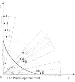
(1) Solutions selected according to the above criteria may contain dominated solutions. Assume there are nine solutions in a population, solutions A to I, for a bi-objective optimization problem, as illustrated in Fig. 1. Suppose that the convergence indicator is the Euclidean distance of a solution to the origin, and the distribution indicator is a vector of the Euclidean distances between this solution to the rest. Clearly, if a solution dominates another, it is very likely to have a better value in terms of the convergence indicator. Assumerαis the distance
threshold to de-emphasize the neighboring solutions once a solution is selected. For the given solutions, A is the first solution to be selected according to the convergence indicator. Then, according to the distribution indicator and the value of
rα, B is de-emphasized. Solution C, which is closer to the origin than solutions D to I, is selected thereafter, although it is dominated by A. By contrast, solution D or F, which are non-dominated by solution A, will not be selected. This means that the selection criterion is not strictly consistent with the Pareto dominance criterion. Although the probability that one solution dominates another is considerably low in a high-dimensional objective space, selection of dominated solutions instead of the non-dominated ones may degrade the search performance of the algorithm.
(2) Euclidean distance is not well suited for measuring dis-tribution in a high-dimensional space. Most existing methods, however, such as niche [38] and k-nearest [11], employ the Euclidean distance to estimate the distribution of solutions, which results in a large number of dominance resistant solu-tions (DRS) [13] in the population. For example in Fig. 1, F-I are all selected since for each of them, the Euclidean distance to each of the others is larger than the threshold. As a matter of fact, G, H, and I are farther away from the Pareto optimal front than some solutions which are in a more crowded region, e.g. B. This issue becomes more serious in a high-dimensional space, since the Euclidean distance has been shown to be inadequate to describe the neighborhood relationship in a high-dimensional space [41].
(3) Boundary solutions may be lost during the evolution. For instance, in Fig. 1, boundary solution E is lost once solution D is selected.
(4) An effective method for determining the right threshold still lacks, which is critical for achieving a good distribution performance. Zhang et al. [21] proposed an adaptive strategy based on information from the population at the previous generation. However, information about the shape of the non-dominated front in the current and previous populations may be misleading before the shape of the true Pareto optimal front becomes clear.
To implement the ideas and resolve the issues discussed above, we propose here a many-objective evolutionary algo-rithm using a one-by-one selection strategy. In the proposed method, individuals (candidate solutions) are first sorted ac-cording to a convergence indicator. In each step, only the individual having the best convergence performance will be
0 f1 f2 C D E I H G F A ra A B
The Pareto optimal front
Fig. 1. An illustration of selecting solutions one by one for a bi-objective problem. In this example, dots A to I indicate solutions in the current population. In this example, the convergence indicator of a solution is its Euclidean distance to the origin, and the distribution indicator is its Euclidean distances to other solutions. Solutions on the arcs denoted by a dotted line have the same value in terms of the convergence indicator.rαis a threshold to de-emphasize neighboring solutions, and the circles denoted by dashed lines are the niches formed byrα. On the basis of the convergence and the distribution indicators, solutions A, C, D, F, G, H and I are selected one by one, and B and E are de-emphasized after A and D are selected, respectively. In addition, the shaded area indicates the dominant region dominated by solution A.
selected. Then, individuals in the neighborhood of the selected one or dominated by the selected one are de-emphasized. To efficiently evaluate the distance between solutions in a high-dimensional space, a distribution indicator based on the cosine similarity is employed. In addition, a boundary maintenance mechanism and a normalization method based on the corner solutions are introduced to ensure a good coverage of the Pareto optimal front and to enhance the algorithm’s ability in solving scaled problems. The detail of 1by1EA will be presented in Section III.
It is worth noting that the knee point driven environmental selection proposed in KnEA [21] can also be seen as a one-by-one selection strategy, however, it is used as a secondary selection criterion in addition to non-dominated sorting pro-posed in NSGA-II [10]. In this work we attempt to present a general framework that utilizes the convergence indicator as the primary selection criterion.
III. THEPROPOSEDMETHOD
A. A General Framework
Algorithm 1 presents the overall framework of the proposed 1by1EA, which is similar to most generational MOEAs. First, an initial parent population, P, is created by randomly generatingNindividuals. Then, mating selection is performed to choose solutions for creating offspring. This process repeats until N offspring individuals are generated, which forms the offspring population, P′. Merge P and P′ to form the com-bined populationQ. Next, the convergence and the distribution indicators of each individual in Q are calculated. Finally,
Algorithm 1 A General Framework of 1by1EA
Require: P (population),N (population size)
1: Initialize(P)
2: while the stopping criterion is not metdo
3: P′ = Mating selection(P)
4: P′′ = Variation(P′)
5: Q=P∪P′′
6: Calculate the convergence indicator c(xi) and distri-bution indicator d(xi)of eachxi∈Q, i= 1, ..., N
7: P =One-by-one selection(Q,c,d)
8: end while
9: return P
the one-by-one selection procedure is implemented to select
N individuals from Q to form the population of the next generation.
In the following, we describe in detail the approaches to calculating the convergence and the distribution indicators, the one-by-one selection strategy, and mating selection, which are three important components in 1by1EA.
B. Calculation of the Convergence and the Distribution Indi-cators
1) The convergence indicator: In calculating the
conver-gence performance of a solution, each objective is equally emphasized and aggregated into a scalar indicator. A general formulation of calculating the convergence indicator can be summarized as follows:
c(x) = agg(f1(x), ..., fM(x)) (2)
There are numerous methods for calculating the conver-gence indicator. In the following, we discuss four metrics, among others, that can measure the convergence performance. The first one is the sum of all the objectives (Sum for short):
c(x) =∑M
m=1fm(x) (3) Sum is one of the simplest and most well-known aggregation functions to convert multiple objectives into a single one. Intuitively, it is well suited for problems whose Pareto optimal fronts are linear. Additionally, it is usually believed to be unable to solve problems with concave Pareto optimal fronts [42]. However, previous studies [43], [44] have shown that with an adaptive weighted strategy, Sum can also work well for these problems. Another study [45] has shown that it can achieve better search performance than other aggregation approaches in many-objective knapsack problems.
The second one is the Chebyshev distance to the ideal point (CdI for short):
c(x) = max
1≤m≤M|fm(x)−z
∗
m| (4)
where z∗ = (z∗1, ..., zM∗ )T is the ideal point, and z∗ m = min
xi∈Q
fm(xi). In contrast to Sum, CdI is believed to be capable
of finding Pareto solutions on concave fronts [42]. Although CdI is not smooth for continuous objectives, it is able to solve discrete problems, e.g., scheduling problems [46]. However,
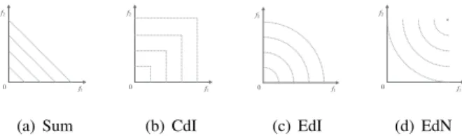
f1 f2 0 (a) Sum f1 f2 0 (b) CdI f1 f2 0 (c) EdI f1 f2 0 (d) EdN Fig. 2. Contour lines formed by different convergence indicators in the bi-objective space.
CdI is widely used in the decomposition-based MOEAs for solving continuous problems [22], [25], [26], since these meth-ods do not need to compute the derivative of an aggregation function. In addition, CdI is usually termed as the achievement function in the preference-based methods to help the decision maker seek his/her favorite solutions [35], [47], [48].
The third one we consider here is the Euclidean distance to an ideal point (EdI for short):
c(x) =√∑M m=1(fm(x)−z ∗ m) 2 (5) Similar to CdI, EdI is advantageous for solving concave problems, especially when their Pareto optimal fronts are a part of hypersphere. It has also been applied in the preference-based methods [39], [49], [50], where the ideal point is usually replaced by a reference point given by the decision maker. In [39], solutions with the smallest values of EdI get the best crowding distances and are preferred in the selection.
The fourth one is the Euclidean distance to the Nadir point (EdN for short):
c(x) = 1 /√∑ M m=1(fm(x)−z nad m ) 2 (6) whereznad= (znad1 , ..., znadM )
T is the nadir point, and
znadm = max
xi∈Q
fm(xi). We employ the reciprocal of the Euclidean distance to the nadir point, since we intend to minimize the convergence indicator. EdN is the invert version of EdI. A recent study [51] has reported that if the distance between the obtainedz∗and the true ideal point is large, evolving solutions towardsz∗ will guide the population toward a specific region of the Pareto optimal front. In such cases, evaluating solutions based on znad may be helpful for approximating the entire Pareto optimal front. EdN is often used in decision making [52], [53], where the solution farthest from the nadir point is the best.
All the above four convergence metrics are computationally cheap and easy to obtain. The contour lines formed by different convergence indicators in the bi-objective space are shown in Fig. 2. Solutions lying on the same contour line have the same value of the convergence indicator. As we discussed above, a convergence indicator is advantageous for problems whose Pareto optimal fronts fit its contour lines. Empirical studies of these convergence indicators have been conducted and the results are presented in the supplementary document. It should be noticed that, different from the preference- and decomposition-based methods, the main advantage of our method is that it does not need any weight/reference vector,
which makes it easier to be applied. Since our aim is not to obtain parts of the Pareto optimal front preferred by the decision maker, it is unnecessary to weight the objectives. In the decomposition-based methods, uniformly [23] or adaptive-ly [24], [27] generating the reference vectors is particularadaptive-ly important to achieve good distribution performance. However, in our method, the distribution issue can be resolved by the niche technique based on a distribution indicator.
2) The distribution indicator: The distribution indicator
is a vector with each of its element indicating the distance between a solution to the rest in the population. Almost all existing distribution performance indicators employ the Euclidean distance to calculate the distance between solutions, or to estimate the solution density. However, as discussed in Section II.B, the Euclidean distance is not well suited for measuring distribution in a high-dimensional space.
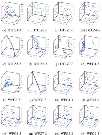
The cosine similarity [54] uses the cosine of the angle between two vectors to measure their similarity. Two vectors with exactly the same orientation result in a cosine similarity of 1, and those which are perpendicular with each other produce a cosine similarity of 0. The cosine similarity is within the range of [0,1] regardless of the dimensionality of the vectors. Therefore, the cosine similarity has widely been used for measuring similarity in a high-dimensional space, e.g., in data mining [54], document clustering [55], and intuitionistic fuzzy sets [56]. For many-objective evolutionary optimization, we hypothesize that the cosine similarity will be more effective in distinguishing two solutions in a high-dimensional space than similarity measures based on the Euclidean distance. Fig. 3 provides an illustrative example, where the distribution indicator is the cosine similarity between a solution and the rest, and cos (θ) is used as the threshold to de-emphasize neighboring solutions. Solution A is first selected, and then C is de-emphasized according to the threshold,cos (θ). Next, so-lutions B and D are selected, and E is de-emphasized. Finally, F is selected, and I, H, G are de-emphasized. Compared to the selection results illustrated in Fig. 1, in which the Euclidean distance is employed as the distribution indicator, this example shows that utilizing the cosine similarity as the distribution indicator is very helpful in reducingDRSs such as solutions G, H, and I.
Therefore, the following distribution indicator is adopted in this study:
d(xi) = (d1(xi), ..., d|Q|(xi)), i= 1, ...,|Q| (7)
where
dj(xi) = 1−cos (θij), j= 1, ...,|Q| (8) is the distance betweenxi andxj, and
cos (θij) = ∑M m=1(fm(xi)−z ∗ m)·(fm(xj)−zm∗) √∑M m=1(fm(xi)−z∗m)2· √∑M m=1(fm(xj)−z∗m)2 (9)
It is worth noting that dj(xi) falls in the range of [0, 1], and the smaller dj(xi), the closer between xi and xj. In
addition, dj(xi) is equal to di(xj), and di(xi) = 0. In the selection process, after solution xi is selected, each xj ∈ Q
0 f1 f2 C D E I H G F A A B
The Pareto optimal front
θθ
θ θ θ θ θθ
Fig. 3. An example of selecting solutions one by one for a bi-objective problem, where the convergence indicator is the Euclidean distance between a solution and the original point, and the distribution indicator is its cosine similarity to each of the others. Solutions on a quarter circle with dotted lines have the same values of the convergence indicator.cos (θ)is the threshold to de-emphasize neighbors, and the sectors with the dashed lines are the niches formed bycos (θ). On the basis of the convergence and the distribution indicators, A, B, D, and F are selected in turn, and C, E, and G-I are de-emphasized after A , D, and F are chosen, respectively.
whose distance with solutionxi, i.e.,dj(xi)is smaller than the
threshold will be de-emphasized. Using the cosine similarity as the distribution indicator, we can resolve the issue mentioned in Section II.B.
It is interesting to note that the distribution indicator based on the cosine similarity has an inherent relationship with the penalty-based boundary intersection (PBI) in MOEA/D [22] and the reference point-based diversity maintenance mech-anism in NSGA-III [20]. Taking Fig. 4 as an example, in MOEA/D with the PBI function and NSGA-III, the distribu-tion performance of soludistribu-tion x is measured by its distance to the reference vector, i.e., d2, which is calculated using the following expression:
d2=|x| ·
√
1−cos2θ (10)
It can be conceived thatd2has similar mathematical properties to the distribution indicator based on the cosine similarity. However, our method does not need any predefined reference vectors and is easy to adapt.
C. The One-by-one Selection Strategy
The one-by-one selection strategy is the key component of 1by1EA, and its detailed procedure is described in Algorithms 2, 3, and 4. Based on the convergence and the distribution indicators, individuals in the combined population, Q, are classified into the following three subsets:Qs, the pre-selected individuals (not necessarily be selected),Qth, the individuals de-emphasized by the distribution threshold, and Qd, the individuals dominated by the selected ones.
First, a boundary maintenance mechanism is performed to preserve the corner individuals, referring to Algorithm 2, lines
f1 f2 0 Re fere nc eV ec tor x G G θ
Fig. 4. The distribution performance of solutions in MOEA/D with PBI and NSGA-III.
Algorithm 2 One-by-one selection(Q,c,d)
Require: N (population size),ζ(distribution threshold to
de-emphasize individuals) 1: P =∅
2: Qs=∅ ◃ set of pre-selected individuals 3: Qth=∅ ◃ set of de-emphasized individuals byζ
4: Qd=∅ ◃ set of dominated individuals
5: nrank= 1 ◃rank used for tournament strategy in mating selection
6: form= 1→M do
7: ifQ̸=∅ then
8: Selecting the unique individual(cm(x))
9: De-emphasizing individuals(xunique,ζ)
10: rank(xunique) =nrank
11: end if
12: end for
13: while Q̸=∅ do
14: Selecting the unique individual(c(x))
15: De-emphasizing individuals(xunique,ζ)
16: rank(xunique) =nrank
17: end while
18: r=|Qs|/N
19: Nd=|Qd|
20: if |Qs| ≥N then
21: P ={xi|xi∈Qs, i≤N} ◃ add the firstN
individuals in Qs toP 22: else 23: while|Qs|< N do 24: if Q=∅ then 25: Q=Qth∪Qd 26: Qth=∅ 27: Qd =∅ 28: nrank=nrank+ 1 29: end if
30: Selecting the unique individual(c(x))
31: De-emphasizing individuals(xunique,ζ)
32: rank(xunique) =nrank
33: end while
34: P =Qs
35: end if
36: ζ=update(ζ, r, Nd)
Algorithm 3 Selecting the unique individual(fagg(x)) 1: xunique= arg min
xi∈Q
fagg(xi)
2: Qs=Qs∪ {xunique}
3: Q=Q\{xunique}
4: returnxunique
Algorithm 4 De-emphasizing individuals(xunique,ζ)
1: for allxi:di(xunique)< ζ,xi∈Qdo
2: Qth=Qth∪ {xi}
3: Q=Q\{xi}
4: end for
5: for allxi:xi≻xunique,xi∈Qdo
6: Qd=Qd∪ {xi}
7: Q=Q\{xi}
8: end for
9: returnQ
6-12. In this study, a corner individual shares a similar concept of the corner solution defined in [57]. If a solution is generated by simultaneously minimizing kc(kc< M) objectives of an
M-objective problem, it is referred to as a corner solution. Following the above definition, a corner individual can be defined to be the individual with the smallest value of a scalar function aggregated bykcobjectives in the current population. Since kc can take values from1 toM−1, there are 2M −1
possible corner solutions lying on the boundaries of the Pareto optimal front. Likewise, there exit 2M −1 possible corner individuals in a population. As a matter of fact, the number of corner solutions lying on the Pareto optimal front is often much fewer. The M corner solutions lying on the objective axes have a good ability in representing the bound of each objective on the Pareto optimal front, and can be obtained by simultaneously minimizing M −1 objectives. Consequently, to achieve the homologous corner individuals, we employ M
aggregated scalar functions that can be termed as variations of the convergence indicator:
cm(x) = agg(f1(x), ..., fm−1(x), fm+1(x)..., fM(x)), (11) m= 1, ..., M For example, cm(x) =√∑M i=1,i̸=m(fi(x)−z ∗ i) 2 , m= 1, ..., M (12) Then the corner individual,xconer
m , can be obtained as follows,
xconerm = arg minx
i∈Q
cm(xi), m= 1, ..., M (13) Prioritizing these corner individuals in selection can enhance the algorithm’s ability in covering the Pareto optimal front as widely as possible. Moreover, these individuals are definitely non-dominated individuals [57]. Out of the above reasons, the corner individuals are first selected and put into Qs.
Next, the rest individuals in Q are chosen to put into Qs
one by one, referring to Algorithm 2, lines 13-17. It should be noted that once an individual is select intoQs(lines 8 and
14 in Algorithm 2), the individuals either near this solution or dominated by this solution will be de-emphasized, as shown in Algorithm 2, lines 9 and 15. As a result, no dominated individuals are chosen before any other non-dominated ones, and the problem mentioned in Item (1) in Section II.B can be solved. These selection and de-emphasizing operators will repeat untilQbecomes empty.
When Q is empty for the first time, if the number of individuals inQsis larger than the predefined population size,
N, only the firstN individuals inQs will be selected intoP
( refer to Algorithm 2, lines 20-21); otherwise, the individuals inQthandQdwill compete to survive untilN individuals are selected into Qs (Algorithm 2, lines 23-33). In this process, onceQis empty, all individuals inQthandQdwill be moved toQ(Algorithm 2, lines 24-29).
Last but not the least, the distribution threshold, ζ, is updated based on the size of Qs (Algorithm 2, line 36) to ensure thatN solutions are selected. The updating method is similar to that used in [21]:
ζt=ζt−1eM1(Rr−1) (14)
where ζt−1 and rt−1 = |Qs|/N (Algorithm 2, line 18) are the distribution threshold and the ratio of the number of pre-selected individuals to the population size at the (t −1) -th generation, respectively. In -this study, ζ1 is set to 1.
R∈[0,2]is a threshold to control the number of pre-selected individuals. Intuitively, whenR= 1, the convergence and the distribution performances can be properly balanced. This will be empirically verified in the experiments in the supplementary document. Due to the adaptation in (14), if the number of pre-selected individuals is smaller than R·N, ζt will decrease,
and vice versa. Thus, the number of pre-selected individuals remains aroundR·N. However, as mentioned in Section II.B, the true Pareto optimal front is unknown during the evolution, implying that it might be misleading to adaptζtbased onrt−1
andζt−1. If the number of dominated individuals in Qd, i.e.
Nd (Algorithm 2, line 19), is larger than (2−R)·N at the
(t−1)-th generation, the number of pre-selected individuals at the (t−1)-th generation cannot be N, regardless of the value of ζt−1. In such case, ζt should remain unchanged if Nd>(2−R)·N.
D. The Mating Selection Strategy
The one-by-one selection strategy described in the previous section is adopted in environmental selection. In the mating selection, a binary tournament selection strategy is proposed to choose promising individuals to form a mating pool. Two tournament strategies are employed, i.e., the ranking method using information from one-by-one selection and the density estimation based on the distribution indicator.
First, two individuals are randomly selected from the parent population. If one has a lower rank than the other, the former is chosen, where the rank, rank(x), can be obtained based on the result of the one-by-one selection at the previous generation. BeforeQbecomes empty, the rank of the solutions chosen intoQsis set to 1 (Algorithm 2, lines 10 and 16). Once
solutions will be increment by 1 (see Algorithm 2, lines 28 and 32). Note that the rank of each individual at the first generation is set to 1.
Next, if these two individuals have the same rank, we prefer the one with a lower density estimation value, dk(x), which is formulated as follows:
dk(x) =∑k 1
i=1dmini (x) + 1
(15) wheredmini (x), i= 1, ..., kis one of theksmallest values in
{
d1(x), ..., d|P|(x)
}
. It can be seen that the density estimation method is a variant of thek-th nearest neighbor method. The difference is that we use the cosine similarity to calculate
dj(x), j= 1, ...|P|, which is the same as in (8), rather than
the Euclidean distance.
Finally, if the density estimation fails to distinguish the two individuals, one of them will be chosen randomly.
E. Normalization Based on the Corner Solutions
In this study, we further incorporate a normalization proce-dure into 1by1EA based on the corner solutions to enhance its ability in solving scaled problems. This version of 1by1EA using corner solution based normalization is termed 1by1EA-norm.
Normalization has been demonstrated to be helpful in solving problems whose objective values are disparately scaled [20], [21], [25], [33], [40]. In the normalization, the objective,
fm(x), m= 1,2, ..., M, is replaced by fm′ (x) = fm(x)−f lb m fub m −fmlb (16) wherefmlbandfmubshould be the lower and the upper bounds of them-th objective on the Pareto optimal front, respectively. Since the Pareto optimal front is unknown, fmlb and fmub are
usually estimated based on the obtained solution set. fmlb can
be easily set to be the minimal value offm(x)in the current population, whereas the estimation offub
m requires information
about the true Pareto optimal front. In 1by1EA-norm, fub
m is estimated based on M corner
individuals. As mentioned in Section III.C, by simultaneously minimizing M −1 objectives, a corner solution lying on the objective axes can be obtained, and the value of the objective that is not minimized can represent the upper bound of the objective on the Pareto optimal front. Thus, the homologous corner individuals are well suited for estimatingfmub, andfmub
as follows:
fmub=fm(xconerm ), m= 1, ..., M (17)
At each generation in 1by1EA-norm, before calculating the convergence and the distribution indicators, each individual in the combined population, Q, will be normalized using (16). It should be noted that after normalization, the ideal point, z∗, used for calculating the convergence and the distribution indicators should be set to(0, ...,0), whereas the value of each element of the nadir point,znad, may be larger than 1. Owing to this normalization procedure, 1by1EA-norm is particularly capable of solving scaled problems, which will be empirically shown in the experiments.
TABLE I
THE CHARACTERISTICS OF THE TEST PROBLEMS,WHEREkwIS THE POSITION-RELATED PARAMETER WHOSE VALUE ISM−1.
Problem n Characteristics DTLZ1 M+4 Linear, Multimodal DTLZ2 M+9 Concave DTLZ3 M+9 Concave, Multimodal DTLZ4 M+9 Concave, Biased DTLZ5 M+9 Concave, Degenerate DTLZ6 M+9 Concave, Degenerate, Biased
DTLZ7 M+19 Mixed, Disconnected, Multimodal, Scaled WFG1 kw+24 Mixed, Biased, Scaled
WFG2 kw+24 Convex, Disconnected, Multi-modal, Non-separable, Scaled
WFG3 kw+24 Linear, Degenerate, Non-separable, Scaled WFG4 kw+24 Concave, Multimodal, Scaled
WFG5 kw+24 Concave, Biased, Scaled WFG6 kw+24 Concave, Non-separable, Scaled WFG7 kw+24 Concave, Biased, Scaled
WFG8 kw+24 Concave, Biased, Non-separable, Scaled WFG9 kw+24 Concave, Biased, Multi-modal, Deceptive,
Non-separable, Scaled
IV. EXPERIMENTALDESIGN
This section describes the experimental design for examin-ing the performance of 1by1EA. The test problems and the performance indicators used in the experiments are given at first. Then, eight state-of-the-art MOEAs to be compared, i.e., KnEA [21], BiGE [40], EFR-RR [25], MOEA/D-ACD [26], MOMBI-II [33], NSGA-III [20], GrEA [29], and SDE [19], are briefly introduced. Finally, the commonly used parameters are set for the comparative studies of these algorithms.
A. Test Problems and Performance Indicators
DTLZ [58] and WFG [59], two widely used test suites, are adopted for empirical comparisons in this study. These test suites are composed of optimization problems having linear, concave, multimodal, disconnected, biased, scaled, or degenerate Pareto optimal fronts. The characteristics of the Pareto optimal front of different test problems are summarized in Table I. In this paper, we consider these problems with 3, 6, 8, 10 and 15 objectives. A detailed description of the DTLZ and WFG suites can be found in [58] and [59].
In order to measure the performance of different algorithms on these test problems, the inverted generation distance plus (IGD+) [60] is adopted in this work. IGD+ is a modified version of IGD [61], which is a widely used performance indicator. IGD can measure both the convergence and diversity performance of a solution set obtained by an algorithm, and the smaller the value of IGD, the better the performance of the algorithm. However, IGD is a Pareto non-compliant indicator, thus it may result in inaccurate evaluation in some cases. In IGD+, the distance between a solution and a reference point is refined by taking their Pareto dominance relationship into account, which makes it weakly Pareto compliant and more accurate on evaluation. Similar to IGD, IGD+ requires a reference set and the reference points are typically uniformly distributed on the Pareto optimal front of a test problem. In this work, we set the number of reference points to around 5,000 and 10,000 when M ∈ {3,6,8,10} and M = 15,
respectively. It should be noticed that when calculating IGD+ for scaled problems, both solutions and reference points will be normalized based on the true Pareto optimal front.
B. Compared Algorithms
The following eight state-of-the-art MOEAs are chosen for comparison to assess the performance of the proposed algorithm: KnEA [21], BiGE [40], EFR-RR [25], MOEA/D-ACD [26], MOMBI-II [33], NSGA-III [20], GrEA [29], and SDE [19]. These algorithms cover all the main categories mentioned in Section I for many-objective optimization. The code of these algorithms except for NSGA-III are all from the authors. NSGA-III is implemented by the authors of KnEA.
• KnEA [21] was established under the framework of NSGA-II [10], and it gives a priority to the knee points among non-dominated solutions. The process of seeking local knee points can also be seen as a one-by-one selec-tion procedure, in which the distance between a soluselec-tion and the hyperplane defined by the extreme solutions is used as the convergence indicator, and the Chebyshev distance between solutions is utilized for the distribution indicator. Hence, KnEA is very relevant to the proposed algorithm.
• BiGE [40] also simultaneously considers the convergence and distribution performance of a solution. Different from 1by1EA, BiGE transforms an MaOP into a bi-objective problem whose objectives are the convergence and distri-bution indicators. A solution set with well-balanced per-formance can be achieved by optimizing the bi-objective optimization problem. However, the niche technique used in BiGE is based on the Euclidean distance and the niche size cannot be tuned adaptively.
• EFR-RR [25] is based on the framework of NSGA-II. However, it is inherently a decomposition-based method like MOEA/D [22]. EFR-RR considers the distribution performance of a solution firstly. Only when the perpen-dicular distance from the solution to the reference vector is small, its scalarizing function value will be calculated. This method suggests another idea on balancing con-vergence and diversity in the high-dimensional objective space and has also been applied to MOEA/D, termed MOEA/D-DU. Since EFR-RR performs slightly better than MOEA/D-DU according to the original study, we choose the former for comparison.
• MOEA/D-ACD [26] was developed from the original MOEA/D. The goal of this method is similar to EFR-RR. However, it achieves this goal by adding constraints to the scalarizing functions. In this way, the angle between a solution and the reference point is limited by a threshold, which guarantees the distribution performance of the solution. Moreover, this method offers a strategy for adaptively adjusting the threshold.
• MOMBI-II [33] is an indicator-based algorithm that uses the R2 indicator to guide the search. The R2 indicator is an attractive alternative to hypervolume [32], due to its low computational cost and weak-Pareto compatibility. MOMBI-II takes two key aspects into account, i.e., using
the scalarizing function and statistical information about the population’s proximity to the true Pareto optimal front.
• NSGA-III [20] was adapted from a popular dominance-based MOEA, II, for handling MaOPs. NSGA-III uses a reference-point-based selection criterion in-stead of a density-based counterpart (crowding distance) in NSGA-II. A two-layer strategy was proposed for generating well-distributed reference points in the high-dimensional objective space, which can also be used in MOEA/D.
• GrEA [29] exploits the potential of the grid-based ap-proach to deal with MaOPs. Grid dominance and grid difference are introduced to determine the relationship between individuals in a grid environment. Three grid-based criteria are incorporated into the fitness of an individual to distinguish individuals in both mating and environmental selection processes. Moreover, a fitness adjustment strategy was developed to avoid partial over-crowding as well as to guide the search towards various directions in the archive.
• SDE [19] is a recently proposed method that modifies the density estimation strategies in traditional Pareto-based MOEAs. By shifting the position of an individual in a sparse region, individuals with poor convergence can be assigned with a high density value, and then discarded during the selection. In this study, the version that inte-grates SDE into SPEA2 [11] (denoted as SPEA2+SDE) is employed due to its better performance compared to other variants.
C. Parameter Settings
The following parameter settings are adopted by all com-pared algorithms. Simulated binary crossover and polynomial mutation are used as the crossover and mutation operators, with both distribution indexes being set to 20. The crossover and mutation probabilities are 1.0 and1/n, respectively, where
n is the number of decision variables. These settings of the evolutionary operators are the same as those in the recent studies and have been demonstrated to be able to generate good solutions [19], [21], [25], [29], [40]. The termination criterion is the predefined maximum number of generations. For difficult problems, i.e., DTLZ1, DTLZ3, DTLZ6 and WFG1, the maximum number of generations is set to 1,000 so that the algorithms are able to converge sufficiently to the true Pareto optimal front. For the other test problems, the maximum number of generations is set to 300. To avoid the situation in which all reference points locate on the boundary of the Pareto optimal front for problems with a large number of objectives, the strategy of two-layered reference points is used for EFR-RR, MOEA/D-ACD, MOMBI-II and NSGA-III. As a result, the population size of EFR-RR, MOEA/D-ACD and NSGA-III cannot be arbitrarily specified. For a fair comparison, we set the population size of the other algorithms under comparison to the same value as these three algorithms. The setting of the population size,N, and the parameters for controlling the number of reference points are listed in Table II.
TABLE II
SETTING OF THE POPULATION SIZE,WHEREp1ANDp2ARE PARAMETERS CONTROLLING THE NUMBER OF REFERENCE POINTS ALONG THE
BOUNDARY OF THEPARETO OPTIMAL FRONT AND INSIDE IT, RESPECTIVELY. M p1 p2 N 3 13 0 105 6 4 1 132 8 3 2 156 10 3 2 275 15 2 1 135 TABLE III
THE PARAMETER SETTINGS INKNEAANDGREA,WHERE THE VALUES OF BOTHTANDdivCORRESPOND TO THE NUMBER OF OBJECTIVES OF A
PROBLEM.
T in KnEA divin GrEA
M 3 6 8 10 15 3 6 8 10 15 DTLZ1 0.5 0.2 0.1 0.1 0.1 11 11 11 13 28 DTLZ2 0.5 0.5 0.5 0.5 0.5 11 8 8 9 10 DTLZ3 0.5 0.2 0.1 0.1 0.1 12 15 15 15 28 DTLZ4 0.5 0.5 0.5 0.5 0.5 11 8 8 9 10 DTLZ5 0.5 0.5 0.3 0.3 0.2 38 16 11 11 12 DTLZ6 0.5 0.4 0.3 0.3 0.2 40 50 50 50 50 DTLZ7 0.5 0.5 0.5 0.4 0.4 10 8 6 4 4 WFG1 0.5 0.5 0.5 0.5 0.5 5 6 8 10 15 WFG2 0.5 0.5 0.5 0.5 0.5 10 9 9 9 17 WFG3 0.5 0.5 0.5 0.5 0.5 18 18 18 24 22 WFG4&9 0.5 0.5 0.3 0.3 0.3 10 11 11 14 12 WFG5-8 0.5 0.5 0.5 0.5 0.5 10 11 11 14 12
In 1by1EA,k is set to 0.1N to balance the computational cost and the accuracy in estimating the density.Ris set to 1 to balance convergence and distribution as discussed in Section III.C. The Sum method is adopted as the convergence indicator for DTLZ1 and WFG3, since they have linear Pareto optimal fronts. The Pareto optimal fronts of DTLZ7, WFG1 and WFG2 are complex, and can be roughly regarded as different hyperplanes. As a result, the Sum method is also applied to these problems. Additionally, EdI is applied to the other problems of DTLZ and WFG, since all these problems are concave. As suggested in the original studies, the Chebychev approach and the PBI approach with θ = 5 are chosen as the scalarizing method in EFR-RR and MOEA/D-ACD, respectively. The neighborhood size is set to 0.1N in both algorithms. Additionally,Kis set to 2 in EFR-RR. Since both the number of objectives and the population size are different from those of the original KnEA and GrEA, we adjust the threshold, T, in KnEA and the grid division, div, in GrEA according to the guidelines provided in the original studies to achieve the best performances of these algorithms. The settings ofT anddivfor DTLZ and WFG problems are listed in Table III.
Each algorithm is run for 20 times on each optimization problem, and the mean value of IGD+are calculated. In addi-tion, the Wilcoxon’s rank sum test is employed to determine whether one algorithm has a statistically significant difference with the other on the performance indicator, and the null hypothesis is rejected at a significant level of 0.05.
0.1 0.2 0.3 0.4 0.5 0.5 0.5 0.1 0.2 0.3 0.4 0.5 0.5 0.5 0.1 0.2 0.3 0.4 0.5 0.5 0.5 (a) DTLZ1-3 0.2 0.4 0.6 0.8 1 1 1 0.2 0.4 0.6 0.8 1 1 1 0.2 0.4 0.6 0.8 1 1 1 (b) DTLZ2-3 0.2 0.4 0.6 0.8 1 1 1 0.2 0.4 0.6 0.8 1 1 1 0.2 0.4 0.6 0.8 1 1 1 (c) DTLZ3-3 0.2 0.4 0.6 0.8 1 1 1 0.2 0.4 0.6 0.8 1 1 1 0.2 0.4 0.6 0.8 1 1 1 (d) DTLZ4-3 0.1 0.2 0.3 0.4 0.5 0.6 0.7 0.1 0.2 0.3 0.4 0.5 0.6 0.7 0.2 0.4 0.6 0.8 1 1 1 (e) DTLZ5-3 0.2 0.4 0.6 0.8 1 1 1 0.2 0.4 0.6 0.8 1 1 1 0.3 0.6 0.9 1.2 1.2 1.2 1.2 (f) DTLZ6-3 0.2 0.4 0.6 0.8 0.8 0.8 0.8 0.2 0.4 0.6 0.8 0.8 0.8 0.8 2.8 3.5 4.2 4.9 5.6 5.6 5.6 (g) DTLZ7-3 0.4 0.8 1.2 1.6 1.6 1.6 1.6 0.8 1.6 2.4 3.2 3.2 3.2 3.2 0.5 1 1.5 2 2.5 2.5 2.5 (h) WFG1-3 0.4 0.8 1.2 1.6 1.6 1.6 1.6 0.8 1.6 2.4 3.2 3.2 3.2 3.2 1 2 3 4 5 5 5 (i) WFG2-3 0.1 0.2 0.3 0.4 0.5 0.6 0.6 0.2 0.4 0.6 0.8 1 1.2 1.2 2.8 3.5 4.2 4.9 5.6 5.6 5.6 (j) WFG3-3 0.4 0.8 1.2 1.6 2 2 2 0.8 1.6 2.4 3.2 4 4 4 1 2 3 4 5 6 6 (k) WFG4-3 0.4 0.8 1.2 1.6 2 2 2 0.8 1.6 2.4 3.2 4 4 4 1 2 3 4 5 6 6 (l) WFG5-3 0.4 0.8 1.2 1.6 2 2 2 0.8 1.6 2.4 3.2 4 4 4 1 2 3 4 5 6 6 (m) WFG6-3 0.4 0.8 1.2 1.6 2 2 2 0.8 1.6 2.4 3.2 4 4 4 1 2 3 4 5 6 6 (n) WFG7-3 0.4 0.8 1.2 1.6 2 2 2 0.8 1.6 2.4 3.2 4 4 4 1 2 3 4 5 6 6 (o) WFG8-3 0.4 0.8 1.2 1.6 2 2 2 0.8 1.6 2.4 3.2 4 4 4 1 2 3 4 5 6 6 (p) WFG9-3 Fig. 5. Pareto fronts achieved by 1by1EA on 3-objective DTLZ and WFG problems.
V. RESULTS ANDDISCUSSIONS
In this section, the performances of 1by1EA are empirically evaluated. The experiments are divided into the following two parts. The first part investigates the achieved Pareto fronts of 1by1EA on 3-objective problems, and the second compares 1by1EA with the other eight state-of-the-art MOEAs.
A. Pareto fronts achieved by 1by1EA on 3-objective DTLZ and WFG problems
Before comparing the proposed 1by1EA with the other algorithms on MaOPs, we visualize the Pareto fronts achieved by 1by1EA on 3-objective DTLZ and WFG problems for better a understanding of its performance. Since DTLZ7 and WFG1-9 are scaled problems, 1by1EA-norm was adopted, whereas the original 1by1EA was adopted on DTLZ1-6. Note that the population size was set to 100 in this subsection. Fig. 5 shows the 3D plots of the final solution sets of a single run in the objective space. This particular run is associated with the result which is the closest to the mean IGD+ value. Note that in this paper, DTLZA-B refers to DTLZAwithB objectives, and WFGA-B has a similar meaning.
It is evident from Fig. 5 that the solutions are very close to the Pareto optimal fronts, and they are distributed in the whole region of the fronts for most problems. Although 1by1EA achieves good performance on some degenerate problems, e.g., DTLZ5 and WFG3, it struggles to converge on DTLZ6 be-cause of bias in its objectives. For the disconnected problems,
e.g., DTLZ7 and WFG1, 1by1EA can obtain all parts of their Pareto front and the solutions are distributed very well on DTLZ7.
B. Comparison with State-of-the-art Algorithms
In this subsection, 1by1EA and 1by1EA-norm are compared with KnEA, BiGE, EFR-RR, MOEA/D-ACD, MOMBI-II, NSGA-III, GrEA, and SDE on DTLZ and WFG with no less than four objectives. We divide these problems into the following two groups. The first group is the normalized problems, i.e., DTLZ1 to 6, and the second is the scaled problems, i.e., DTLZ7 and WFG1 to 9.Tables IV and VI show the ranks of different algorithms in terms of their mean values
of IGD+on the normalized problems and the scaled problems,
respectively, where the results with higher ranks are shaded
more brightly. ‘†’ and ‘‡’ indicate that the result is significantly
different from that of 1by1EA and 1by1EA-norm, respectively,
and ‘∗’ suggests that the result is significantly different from
both of them. At the bottom of Tables IV and VI, the average rank (denoted by Avg.Rk) of each algorithm are also given, where the significance test are based on the ranks on each instance. Tables V and VII list the summary of the significance
tests on IGD+ between 1by1EA (1by1EA-norm) and the
other algorithms under comparison. When A vs. B, ‘+’
(‘-’) indicates the number of instances on which the results of
A are significantly better (worse) than those of B, and ‘=’
means the number of instances where there exists no statistical
significance between the results of A and B. The detailed
values of IGD+are provided in the supplementary document.
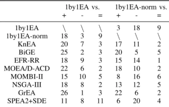
TABLE V
SUMMARY OF THE SIGNIFICANCE TEST OFIGD+BETWEEN THE
PROPOSED ALGORITHMS AND THE OTHER ALGORITHMS ONDTLZ1TO6.
1by1EA vs. 1by1EA-norm vs. + - = + - = 1by1EA \ \ \ 3 18 9 1by1EA-norm 18 3 9 \ \ \ KnEA 20 7 3 17 11 2 BiGE 25 2 3 20 5 5 EFR-RR 18 9 3 15 14 1 MOEA/D-ACD 22 6 2 18 10 2 MOMBI-II 15 10 5 8 16 6 NSGA-III 18 8 2 13 12 5 GrEA 26 1 3 22 6 2 SPEA2+SDE 11 8 11 6 20 4
From Tables IV- VII we can draw the following conclu-sions. Generally, 1by1EA and 1by1EA-norm perform best on the normalized and scaled problems, respectively, among the ten compared algorithms, according to their average ranks.
Although the statistical analysis in terms of rank does not show that 1by1EA (1by1EA-norm) has a significant better performance than the second and the third best algorithms, we can see from Table V ( VII) that 1by1EA (1by1EA-norm) significantly outperforms them on most test instances.
Since the original 1by1EA lacks the normalization procedure, it does not work as well as 1by1EA-norm on the scaled problems, demonstrating the effectiveness of the normaliza-tion procedure for scaled problems. By contrast, 1by1EA-norm does not behave as well as 1by1EA on the 1by1EA-normalized
TABLE VII
SUMMARY OF THE SIGNIFICANCE TEST OFIGD+BETWEEN THE
PROPOSED ALGORITHMS AND THE OTHER ALGORITHMS ONDTLZ7AND
WFG1TO9. 1by1EA vs. 1by1EA-norm vs. + - = + - = 1by1EA \ \ \ 42 7 1 1by1EA-norm 7 42 1 \ \ \ KnEA 9 39 2 27 15 8 BiGE 14 36 0 24 16 10 EFR-RR 9 39 2 26 16 8 MOEA/D-ACD 47 1 2 50 0 0 MOMBI-II 20 25 5 42 6 2 NSGA-III 12 35 3 25 16 9 GrEA 7 36 7 26 14 10 SPEA2+SDE 7 37 6 33 11 7
problems, because the normalization procedure may transform the original objectives into wrong scales when solving a normalized problem, especially if the problem has a huge number of local PFs, e.g., DTLZ1 and DTLZ3. It is inter-esting to note that 1by1EA (1by1EA-norm) shows a clearly better performance on DTLZ5 (WFG3). DTLZ5 (WFG3) has
M−1 redundant objectives, and its Pareto optimal front is a degenerate curve (line). Previous studies [62] have shown that the corner solutions are effective for dimensionality reduction. In 1by1EA (1by1EA-norm), solutions are located within the boundaries formed by the corner solutions, which has the same effect as dimensionality reduction. That is why 1by1EA (1by1EA-norm) outperforms the others on DTLZ5 (WFG3). It is worth mentioning that although DTLZ5 and DTLZ6 have the same Pareto optimal front, 1by1EA cannot produce satisfactory results on the latter, since the bias in DTLZ6 objectives results in wrong corner solutions. This phenomenon can be observed visually in Fig. 5(f).It is also interesting to compare the other results on 3-objectives problems in Fig. 5 with those in Tables IV and VI, where 1by1EA (1by1EA-norm) achieves relatively good performance on DTLZ2, 3, 4, 5 and WFG3, 4, 5, 8, 9.
KnEA has an advantage of approximating the Pareto optimal front by giving preferences to the knee points among non-dominated solutions. It has a normalization procedure based on the minimal and the maximal objectives of the current popula-tion. This normalization procedure makes KnEA competitive on the scaled problems. However, it also makes KnEA worse than 1by1EA-norm on DTLZ1 to 6.
BiGE achieves poor IGD+values on the problems that have a large range of objectives, e.g., DTLZ1 and DTLZ3. The main reason is that BiGE uses a niche technique based on the Euclidean distance, and the niche size is not adjustable. However, because of its normalization procedure, it works well on most scaled problems, especially WFG2.
EFR-RR can effectively deal with both the normalized and the scaled problems except for DTLZ5, DTLZ6 and WFG3. This attributes to the fact that the reference vectors employed in EFR-RR are uniformly distributed in the whole objective space, whereas the Pareto optimal solutions of these problems are not. Thus, the performance of EFR-RR can be further improved by integrating a strategy for adaptively generating
TABLE IV
RANKS OF DIFFERENT ALGORITHMS ONDTLZ1TO6IN TERMS OF MEAN VALUES OFIGD+.
Objective 3 6 8 10 15 3 6 8 10 15 3 6 8 10 15 3 6 8 10 15 3 6 8 10 15 3 6 8 10 15 3 6 8 10 15 3 6 8 10 15 3 6 8 10 15 3 6 8 10 15 DTLZ1 5‡ 2‡ 5‡ 5‡ 4‡ 9† 7† 7† 6† 6†8* 8* 9* 8* 8* 10* 10* 10* 10* 9* 4 4* 1* 1* 2* 6* 6* 3* 2* 3* 2 5* 6† 7†7* 1*3‡ 2* 4* 5* 7* 9* 8* 9* 10*3‡ 1‡4* 3* 1* DTLZ2 2 4 4 7‡ 6‡ 5 1 3 3† 1†9* 7* 8* 8* 3* 10* 9* 9* 5 4‡ 4* 8* 6*4‡2* 7* 10* 10* 10* 10* 3* 3 1* 1†9* 1 2 2† 2†8*6† 5‡7* 9*7‡ 8* 6* 5 6‡ 5‡ DTLZ3 3‡ 2‡ 1‡ 3‡ 1 6† 5† 5† 5† 3 7* 7* 8* 8* 10* 9* 10* 10* 10* 8* 5* 9* 4* 1‡4* 10* 8* 6* 6* 6* 1* 1‡ 2‡ 4†5* 2 3* 7* 7* 7* 8* 6* 9* 9* 9* 4* 4‡ 3‡ 2‡ 2 DTLZ4 4‡ 3‡ 3‡ 4‡ 7 7† 9† 9† 7† 5 3‡ 4‡ 6*5‡3* 6*6† 5†10* 4* 1* 1* 1* 2* 1* 2* 6 10* 9* 10* 5* 5* 2‡1* 2* 9* 10* 7* 3* 8* 10*2‡7*8†9* 8* 8* 4‡6* 6 DTLZ5 1‡ 1‡ 1‡ 1‡ 1‡ 6† 8† 4† 3† 8†4*7† 5* 5*5† 10†4* 6* 6* 6* 7* 10* 7* 7* 4* 9* 2 2* 2* 2* 8* 6* 9* 10* 9* 5* 9* 10* 9* 7* 3* 5* 8* 8* 10* 2* 3* 3* 4†3* DTLZ6 7 6 4 6 6‡ 8 7 5 5 1†1* 3* 2* 3* 4* 6* 5 6* 7* 7* 10* 10* 10* 10* 9* 9* 8* 7* 1* 3* 3* 2* 3* 4* 5* 2* 4* 8* 8* 8* 4* 9* 9* 9* 10* 5* 1* 1* 2* 2* Avg.Rk
MOMBI-II NSGA-III GrEA SPEA2+SDE
1by1EA 1by1EA-norm KnEA BiGE EFR-RR MOEA/D-ACD
3.63‡ 5.46† 5.86† 7.56* 4.96† 6.16† 4.36‡ 5.43† 7.63* 3.83‡
TABLE VI
RANKS OF DIFFERENT ALGORITHMS ONDTLZ7ANDWFG1TO9IN TERMS OF MEAN VALUES OFIGD+.
Objective 3 6 8 10 15 3 6 8 10 15 3 6 8 10 15 3 6 8 10 15 3 6 8 10 15 3 6 8 10 15 3 6 8 10 15 3 6 8 10 15 3 6 8 10 15 3 6 8 10 15 DTLZ7 4‡ 4‡ 2‡ 4‡ 4‡ 8† 5† 7† 7† 1† 2†2* 4‡ 6†9* 6* 8* 8* 8* 6* 7* 9* 3‡2* 2* 10* 10* 10* 10* 10*9‡7* 9* 9* 5* 5* 6* 6 5* 3‡ 3‡1*5‡3* 7* 1* 3* 1* 1* 8* WFG1 8‡ 5‡ 4‡ 3‡ 3 7† 6† 6† 4† 2 3* 4* 5 7* 9* 9* 9* 9* 8* 8* 4* 7* 7* 6* 1* 10* 10* 10* 10* 10* 1* 1* 1* 1* 4* 5* 8* 8* 9* 7* 6* 2* 2*5†6* 2* 3* 3‡ 2†5* WFG2 9‡ 9‡ 9‡ 8‡ 5‡ 5† 6† 6† 5† 2†2* 3* 2* 7* 7* 3* 1* 1* 1*1† 8* 5* 3*2† 6‡10* 10* 10* 10* 9* 7‡ 7†7*4†10* 6* 8* 8‡9* 3* 4* 2*4† 6†8* 1* 4* 5† 3† 4‡ WFG3 9‡ 3‡ 3‡ 2‡ 2‡ 1† 1† 1† 1† 1†7* 5* 7* 7* 9* 5* 4* 4* 4* 4* 6* 8* 5* 5* 5* 10* 10* 10* 10* 10* 2* 7* 9* 9* 7* 8* 9* 6* 6* 6* 4* 2* 2* 3‡3* 3* 6* 8* 8* 8* WFG4 9‡ 8‡ 9‡ 9‡ 7‡ 1† 1† 4† 5† 5†7* 6* 6* 4†2* 4* 4*2†2* 3* 3* 2* 1†1* 4* 10* 10* 10* 10* 9* 5* 9* 8* 8* 10* 6* 3* 3† 3†1* 8* 5* 5* 7* 8* 2* 7* 7* 6*6‡ WFG5 9‡ 8‡ 9‡ 9‡ 6‡ 3† 3† 6† 6† 5†6* 6* 4†5* 2* 5*5† 5†3* 4* 8* 4* 2†2* 3* 10* 10* 10* 10* 9* 7* 9‡8* 8* 10*1†1* 1* 1* 1* 4† 2† 3† 4†7* 2†7* 7* 7* 8* WFG6 9‡ 8‡ 9‡ 9‡ 8‡ 5† 1† 3† 6† 5† 8†6* 6* 4* 2* 6†4*4†2* 4* 7†5*2†3* 1*10‡10* 10* 10* 9* 3* 9* 8* 7* 10* 4*2† 1* 1* 3* 2* 3* 5* 5* 6* 1* 7* 7* 8* 7* WFG7 9‡ 9‡ 9‡ 9‡ 8‡ 5† 2† 5† 6† 5†6* 6* 6†5* 2* 8* 5* 4* 3* 3* 7* 4* 1* 2*4† 10‡10* 10* 10* 9* 4* 8‡8* 8* 10*3† 3† 2* 1* 1* 2* 1 3* 4*7‡ 1* 7 7* 7*6‡ WFG8 9‡ 8‡ 9‡ 9‡ 8‡ 2† 1† 1† 1† 1†8* 7* 5* 3* 3* 7* 5* 2* 2†5* 5* 4* 4* 4* 6* 10* 10* 10* 10* 9* 6* 9* 8* 7‡10* 4*2† 3* 6* 2*3†3* 6* 8*7‡ 1† 6* 7* 5* 4* WFG9 9‡ 8‡ 9‡ 9‡ 6‡ 1† 1† 3† 4† 5†5* 4* 6* 5†4*2† 2† 2†1* 3* 6* 5* 1† 2†2* 10* 10* 10* 10* 9* 7* 9* 8* 8* 10* 8* 6* 5* 3†1* 3* 3*4†6*8‡ 4* 6* 7* 7*7‡ Avg.Rk 9.86‡
1by1EA 1by1EA-norm KnEA BiGE EFR-RR MOEA/D-ACD
7.08‡ 3.68† 5.12* 4.36† 4.12‡ 7.10‡ 4.26† 4.40* 5.00*
MOMBI-II NSGA-III GrEA SPEA2+SDE
the reference vectors [24], [27].
MOEA/D-ACD achieves appealing results on normalized problems. We notice that the number of non-dominated so-lutions in the final set is fewer than the population size in most cases, which makes MOEA/D-ACD less advantageous. In addition, MOEA/D-ACD performs poorly on all scaled problems. This does not mean that MOEA/D-ACD is ineffec-tive for dealing with MaOPs. The main reason is that it lacks a normalization procedure, which confirms that normalization is particularly important in solving scaled problems.However, 1by1EA without normalization also significantly performs better than MOEA/D-ACD on scaled problems.
Although MOMBI-II has a normalization procedure, it performs relatively well on most normalized problems. This can be attributed to its advanced strategy for updating the nadir point, which reduces the risk of transforming the original objectives to wrong scales. However, MOMBI-II does not achieve satisfactory results on the scaled problems except for WFG1.
NSGA-III shows an overall competitive performance on both the normalized and scaled problems except for DTLZ5, DTLZ6 and WFG3 due to the same weakness of EFR-RR. Moreover, since DTLZ4 has a non-uniform Pareto optimal front, NSGA-III cannot maintain a good diversity like EFR-RR.
GrEA achieves encouraging results on most scaled problems and some low-dimensional normalized problems. By dividing each dimension of the objective space into the same number of divisions, GrEA has an inherent ability of normalization. The main drawback of GrEA is that its performance is very sensitive to the value of parameterdiv. In our experiments, we have tested a number of settings of div for each instance to make sure that GrEA can obtain a satisfactory performance. If a method of adaptively adjustingdivcan be further developed,
the performance of GrEA will be considerably enhanced on various problems.
SPEA2+SDE works quite well on most normalized prob-lems, and generally has the medium performance on the scaled problems among the compared algorithms. However, it works relatively poorly for the scaled problems with more than 3 objectives. We speculate that the bias in the objectives and the high-dimensional objective space make the shifting procedure less efficient in estimating the density of solutions. This remains to be examined in future work.
As a whole, 1by1EA and 1by1EA-norm outperform the compared algorithms on the normalized and scaled problems, respectively. It is worth noting that the normalization proce-dure has a great influence on most existing algorithms. Hav-ing incorporated the normalization procedure, 1by1EA-norm, KnEA, BiGE, EFR-RR, NSGA-III, and GrEA perform well on scaled problems, but relatively poorly on normalized problems. On the other hand, 1by1EA, MOEA/D-ACD and SPEA2+SDE behave in an opposite way. The normalization procedure in MOMBI-II is inspiring, but needs further investigation. Hence, when and how to apply the normalization procedure is an important issue for future studies in many-objective optimization. Notwithstanding this, for the normalized prob-lems, 1by1EA-norm performs consistently better compared to KnEA, BiGE, MOEA/D-ACD and GrEA. For the scaled problems, the original 1by1EA performs better than MOEA/D-ACD. Moreover, unlike KnEA and GrEA, 1by1EA (1by1EA-norm) is relatively insensitive to its parameters and does not require the generation of reference vectors as required in EFR-RR, MOEA/D-ACD, MOMBI-II and NSGA-III. Therefore, we can conclude that 1by1EA (1by1EA-norm) is very competitive compared with the state-of-the-art of many-objective evolu-tionary algorithms.