Interactive visualization of information hierarchies and applications on the web

Rowan University Rowan University

Rowan Digital Works

Rowan Digital Works

12-31-2007

Interactive visualization of information hierarchies and

Interactive visualization of information hierarchies and

applications on the web

applications on the web

Rowan University

Follow this and additional works at: https://rdw.rowan.edu/etd Part of the Electrical and Computer Engineering Commons

Let us know how access to this document benefits you -

share your thoughts on our feedback form.

Recommended Citation Recommended Citation

Santiago, Confesor III, "Interactive visualization of information hierarchies and applications on the web" (2007). Theses and Dissertations. 840.

https://rdw.rowan.edu/etd/840

This Thesis is brought to you for free and open access by Rowan Digital Works. It has been accepted for inclusion in Theses and Dissertations by an authorized administrator of Rowan Digital Works. For more information, please

Interactive Visualization of Information Hierarchies and Applications on the Web

by

Confesor Santiago III

A Thesis Submitted to the

Graduate Faculty in Partial Fulfillment of the

Requirements for the Degree of

MASTER OF SCIENCE

Department: Electrical and Computer Engineering

Major:

Engineering (Electrical Engineering)

Approved:

Members of the Committee

In Charge of Major Work

Rowan University

Glassboro, New Jersey

ABSTRACT

Confesor Santiago III

INTERACTIVE VISUALIZATION OF INFORMATION HIERARCHIES AND APPLICATIONS ON THE WEB

2007/05

Advisor: Dr. Adrian Rusu Master of Science in Engineering

The visualization of information hierarchies is concerned with the presentation of abstract hi-erarchical information about relationships between various entities. It has many applications in diverse domains such as software engineering, information systems, biology, and chemistry. Infor-mation hierarchies are typically modeled by an abstract tree, where vertices are entities and edges represent relationships between entities. The aim of visualizing tree drawings is to automatically

produce drawings of trees which clearly reflect the relationships of the information hierarchy. This thesis is primarily concerned with problems related to the automatic generation of area-efficient grid drawings of trees, interactively visualizing information hierarchies, and applying our techniques on Web data.

The main achievements of this thesis include:

1. An experimental study on algorithms that produce planar straight-line grid drawings of binary trees,

2. An experimental study that shows the algorithm for producing planar straight-line grid draw-ings of degree-d trees with n nodes with optimal linear area and with user-defined arbitrary

aspect ratio, works well in practice,

3. A rings-based technique for interactively visualizing information hierarchies, in real-time,

4. A survey of Web visualization systems developed to address the "lost in cyberspace" problem,

5. A separation-based Web visualization system that we present as a viable solution to the "lost in cyberspace" problem,

6. A rings-based Web visualization system that we propose as a solution to the "lost in cy-berspace" problem.

To my paternal grandparents, Confesor Sr. and Margarita,

for their care, love, and prayers, and in the everlasting memory

ACKNOWLEDGMENTS

First and foremost, I would like to thank God for this opportunity. May it be known that my works and achievements were only possible through You, and let all glory and honor be Yours in the name of Jesus Christ.

I would like to express my deep appreciation to my major advisor, Dr. Adrian Rusu, for his clear guidance, encouragement, wise counsel, and unwavering support over the past few years. His influence has been invaluable in my development as a researcher, and as a person. It is his continuous help, motivation, and insightful advice that made this thesis possible. I also want to show my respects to him for his incredible enthusiasm for research. Many thanks for supporting me as a Research Assistant. I will always be grateful for the opportunities he created for me. His hard work and dedication to me, as well as other students will never be forgotten.

Many thanks to Dr. Shreekanth Mandayam and Dr. Ganesh Baliga for being in my thesis committee. Their time and comments on my research work is greatly appreciated.

I would like to thank members of Software Engineering, Visualization, and Graphics (SEGV) Research Group including Mr. Chu Yao, Mr. Christopher Clement, and Mr. Christopher Reyes, for their help and effort. Also, I would like to thank Mr. Radu Jianu for his contributions to my research.

I would like to thank the Department of Computer Science and the Center for Innovation and Entrepreneurship for funding my Graduate Assistantship. I would like to thank Dr. Jay Kuder and Dr. Thomas Bryant, their efforts made our patent possible. Also, I would like to thank Dr.

Anthony Marchese providing funds to assist with the patent through the Rowan Undergraduate Venture Capital Fund.

Special thanks to my fiance, Leigh-Anna, for her support through every aspect of everyday life, unconditional love, and companionship, to my parents, Confesor Jr. and Barbara, for providing everything I needed and always being there for me, to my aunt, Margarita, for her prayers and cooking that cheers me up, to my grandfather, Confesor Sr., for being such a good role model, to my grandmother, Margarita, for her love and prayers, to my sister, Antonia, for being a good little sister and always being a friend growing up, to my future in-laws, for their support and treating my like family, and to my close friends, Mark, Andrew, and Ragon for being like brothers to me.

TABLE OF CONTENTS LIST OF FIGURES... x LIST OF TABLES... xv 1. INTRODUCTION... 1 1.1 Information Hierarchies...1 1.2 Tree Drawing ... 1

1.3 Tree Drawing Conventions... 2

1.3.1 Grid Drawings... 2

1.3.2 Planar Drawings ... 3

1.3.3 Straight-line Drawings... 4

1.3.4 Subtree Separation ... 4

1.4 Lost in Cyberspace ... 5

1.5 Contributions and Outline of This Thesis... 5

2. GRID DRAWINGS

OF

2.1 Introduction ... 7

2.2 The Drawing Algorithms Under Evaluation... 10

2.3 Experimental Setting ... 15

2.3.1 Input File Format ... 15

2.3.2 Load/Save Routines... 16

2.3.3 Test Suite ... 18

2.3.4 Quality Measures... 21

2.4 Experimental Analysis...23

2.4.1 Comparison Analysis... ..- 23

2.4.2 Conclusions ... 39

2.5 Charts of Experimental Results... 44

3. A PRACTICAL ALGORITHM FOR PLANAR STRAIGHT-LINE GRID DRAWINGS OF GENERAL TREES WITH LINEAR AREA AND ARBITRARY ASPECT RATIO ... 67

3.1 Introduction ... ... ... 67

3.2 Preliminaries ... 69

3.3 Practical General Tree Drawing Algorithm ... 71

3.3.1 Split Tree... ... 71

3.3.2 Assign Aspect Ratios... 74

3.3.3 Draw Partial Trees... 77

3.3.4 Compose Drawings... 77

3.4 Experimental Results... 83

4. INTERACTIVE VISUALIZATION OF INFORMATION HIERARCHIES ... 88

4.1 Introduction ... 88

4.2 Separation-Based Visualization System ... 89

4.2.1 Separation-Based Drawing Algorithm ... 89

4.2.2 Interaction Strategy ... 90

4.3 Rings-Based Visualization System... 92

4.3.1 Rings-Based Drawing Algorithm ... ... 93

4.3.3 Labeling Method ... 99

4.3.4 Real-Time ... 101

4.3.5 Synchronization ... 101

5. SURVEY OF WEB VISUALIZATIONS... 102

5.1 Introduction... ... 102

5.2

6. REAL-TIME SPACE-EFFICIENT SYNCHRONIZED TREE-BASED WEB VISUAL-IZATION AND DESIGN... 115

6.1 Introduction ... 115

6.2 Separation WebVis ... 118

6.2.1 Crawler... 118

6.2.2 Visualization ... 119

6.2.3 Label Method Extension...120

6.3 Web Global Positioning System... 121

6.3.1 Browser (Detailed Visualization Window) ... 123

6.3.2 Crawler... 124 6.3.3 Visualization ... 126 6.4 Real-Time... 127 6.5 Synchronization... 128 6.6 Users... 129 6.7 User Study... 131 6.7.1 Procedure...131 6.7.2 Timed Results... 134

6.7.3 Subjective Ratings... 136 6.8 New Features ... 137 6.8.1 Variable Depth...:.. 138 6.8.2 Color Coding ... 138 6.8.3 Empty Pages ... 141 6.8.4 Multi-level Navigation... 143 6.8.5 Visualization Favorites... 143

7. CONCLUSION AND FUTURE WORK... 145

LIST OF FIGURES

1.1 Grid drawings of the same tree: (a) straight-line; (b) polyline; (c) non-planar. The root of the tree is shown as a shaded circle, whereas other nodes are shown as black circles. . 3

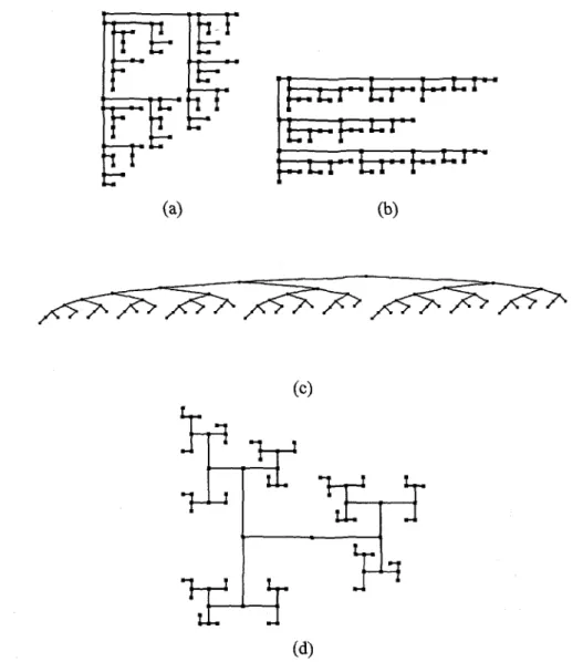
2.1 Drawings of the Fibonacci tree with 88 nodes, generated by the algorithms in our study: (a) Separation, (b) Path, (c) Level, and (d) Rings. ... 11 2.2 Drawings of an unbalanced-to-the-left binary tree with 100 nodes generated by the

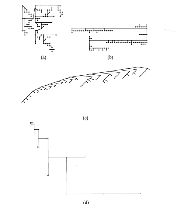
al-gorithms in our study: (a) Separation, (b) Path, (c) Level, and (d) Rings. For Rings, the tree is of size 25 ... 12 2.3 Drawings of an unbalanced-to-the-right binary tree with 100 nodes generated by the

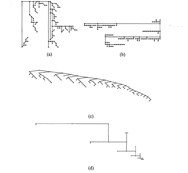
algorithms in our study: (a) Separation, (b) Path, (c) Level, and (d) Rings. For Rings, the tree is of size 25. ... ... . ... 13 2.4 Comparison charts of the area for Level, Path, Rings, and Separation, for each

tree-type: (a) Complete binary trees, (b) AVL trees, (c) Randomly-generated binary tree, (d) Fibonacci trees, (e) Unbalanced-to-the-left binary trees, (f) Unbalanced-to-the-right binary trees, (g) Molecular Combinatory binary trees. ... 46 2.5 Comparison charts of the aspect ratio for Level, Path, Rings, and Separation, for each

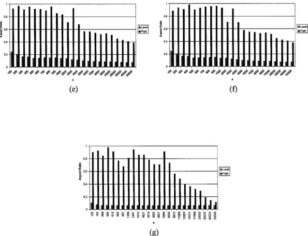
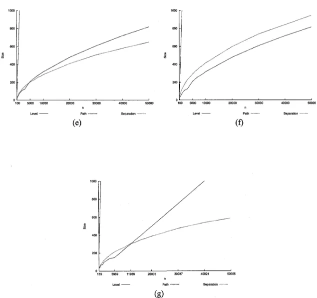
tree-type: (a) Complete binary trees, (b) AVL trees, (c) Randomly-generated binary tree, (d) Fibonacci trees, (e) Unbalanced-to-the-left binary trees, (f) Unbalanced-to-the-right binary trees, (g) Molecular Combinatory binary trees ... 48 2.6 Comparison charts of the size for Level, Path, Rings, and Separation, for each

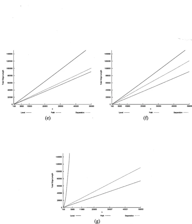
tree-type: (a) Complete binary trees, (b) AVL trees, (c) Randomly-generated binary tree, (d) Fibonacci trees, (e) Unbalanced-to-the-left binary trees, (f) Unbalanced-to-the-right binary trees, (g) Molecular Combinatory binary trees ... 50 2.7 Comparison charts of the total edge length for Level, Path, Rings, and Separation, for

each tree-type: (a) Complete binary trees, (b) AVL trees, (c) Randomly-generated bi-nary tree, (d) Fibonacci trees, (e) to-the-left bibi-nary trees, (f) Unbalanced-to-the-right binary trees, (g) Molecular Combinatory binary trees ... 52

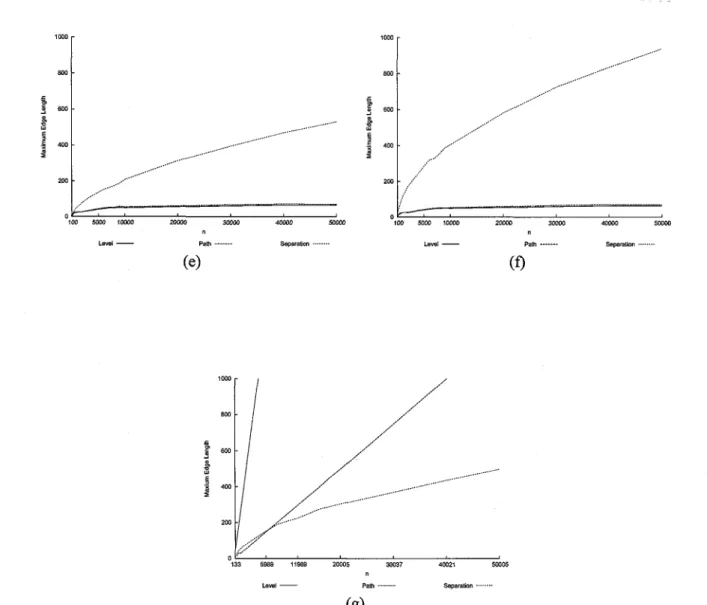
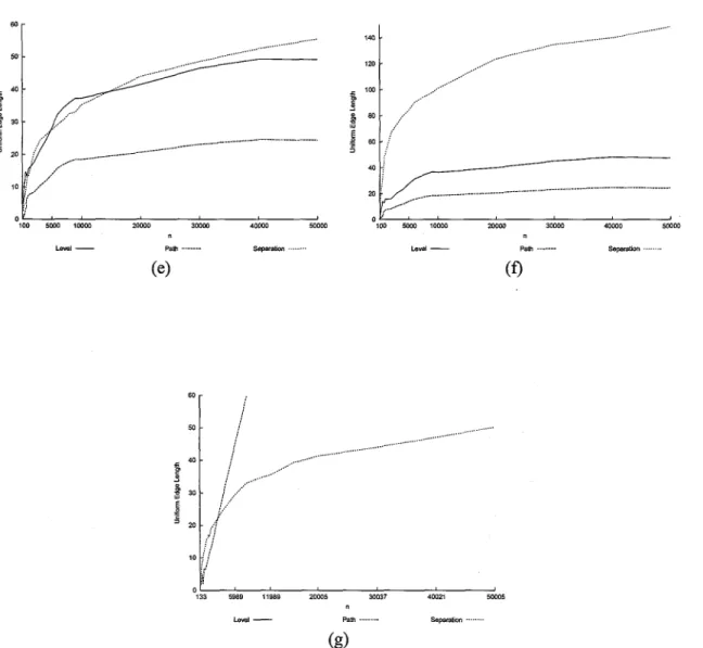
2.8 Comparison charts of the maximum edge length for Level, Path, Rings, and Separation, for each tree-type: (a) Complete binary trees, (b) AVL trees, (c) Randomly-generated binary tree, (d) Fibonacci trees, (e) to-the-left binary trees, (f) Unbalanced-to-the-right binary trees, (g) Molecular Combinatory binary trees ... 54 2.9 Comparison charts of the uniform edge length for Level, Path, Rings, and Separation,

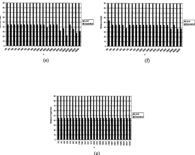
for each tree-type: (a) Complete binary trees, (b) AVL trees, (c) Randomly-generated binary tree, (d) Fibonacci trees, (e) to-the-left binary trees, (f) Unbalanced-to-the-right binary trees, (g) Molecular Combinatory binary trees ... 56 2.10 Comparison charts of the minimum angle size for Level, Path, Rings, and Separation,

for each tree-type: (a) Complete binary trees, (b) AVL trees, (c) Randomly-generated bi-nary trees, (d) Fibonacci trees, (e) to-the-left bibi-nary trees, (f) Unbalanced-to-the-right binary trees, (g) Molecular Combinatory binary trees ... 58 2.11 Comparison charts of the average angle size for Level, Path, Rings, and Separation, for

each tree-type: (a) Complete binary trees, (b) AVL trees, (c) Randomly-generated bi-nary trees, (d) Fibonacci trees, (e) to-the-left bibi-nary trees, (f) Unbalanced-to-the-right binary trees, (g) Molecular Combinatory binary trees. ... 60 2.12 Comparison charts of the angular resolution for Level, Path, Rings, and Separation, for

each tree-type: (a) Complete binary trees, (b) AVL trees, (c) Randomly-generated bi-nary trees, (d) Fibonacci trees, (e) to-the-left bibi-nary trees, (f) Unbalanced-to-the-right binary trees, (g) Molecular Combinatory binary trees ... 62 2.13 Comparison charts of the closest leaf for Level, Path, Rings, and Separation, for each

tree-type: (a) Complete binary trees, (b) AVL trees, (c) Randomly-generated binary trees, (d) Fibonacci trees, (e) the-left binary trees, (f) Unbalanced-to-the-right binary trees, (g) Molecular Combinatory binary trees. ... 64 2.14 Comparison charts of the farthest leaf for Level, Path, Rings, and Separation, for each

tree-type: (a) Complete binary trees, (b) AVL trees, (c) Randomly-generated binary trees, (d) Fibonacci trees, (e) the-left binary trees, (f) Unbalanced-to-the-right binary trees, (g) Molecular Combinatory binary trees ... 66 3.1 Rotating a drawing F by 90°, followed by flipping it vertically. Note that initially node

u* was located at the bottom boundary of F, but after the rotate operation, u* is on the right boundary of F . ... 70 3.2 Drawing of a randomly-generated general tree with 60 nodes constructed by Algorithm

3.3 Drawing T in all the seven subcases of Case 1 (when the separator node u is not in the

leftmost path of T): (a) TA#O, TC Z 0,g=, u*, 0O<i<d-3, (b) TA=0, Tc=0,

0<i<_d- -3, (c) TA C 0,TC 0 ,gg =u*, 0 <i Id- 3,(d) TA =A 0,TC = 0,r e,

0<i< d-3, (e)TA#0 , Tc=0, e, 0< i<d-3,(f)TA =0, Tc Z0,g Z u*,

0 < i < d 3, and (g) TA = 0, Tc = 0, g = u*, 0 < i < d 3. For each subcase, we -first show the structure of T for that subcase, then its drawing when A < 1, and then its drawing when A > 1. Here, x is the same as f if Tp

4)

0,

of Ta if TR =

0.

of FA, but actually, either it is the same as r, or if A < 1 (A > 1), then it is placed on

the bottom (right) boundary of A. For simplicity, we have shown A, TB, and

rC

identically sized boxes, but in actuality, they may have different sizes. ... 75

3.4 Drawing T in all the eight subcases of Case 2 (when the separator node u is in the leftmost path of T): (a)TA#0A TC # ,v f u*,1 <jd 2,(b)TA =0,TC#A 0,v#u*,

S0,

f

#

#

-

1

Tc

#

i

#

#

0

3.5 Drawing Ta. Here, we first show the structure of T, in (a), then its drawing when A < 1 in (b), and then its drawing when A > 1 in (c). ... 78

3.6 Drawing TB when: (a) TR #A 0, and (b) TR = 0. For each case, we first show the structure of TB for that case, then its drawing when A < 1, and then its drawing when A > 1. In Case (a), for simplicity, w is shown to be in the interior of T', but actually, it is either same as f, or ifA < 1 (A > 1), then is placed on the bottom (right) boundary ofrp. ... 78

3.7 Performance of the algorithm, as given by the value of c, for drawing a randomly-generated general tree T with different values of A and e, where c = area of drawing/number of nodes n in T: (a) E = 0.9, (c) E = 0.75, (e) E = 0.5, (g) P = 0.25, and (i) e = 0.1. Figures (b), (d), (f), and (h) contain the projections on the XZ-plane of the plots shown in Figures (a), (c), (e), and (g), respectively, and show for each $, the ranges of the values of c for different values of A for each n. The XZ-plane for E = 0.1 is not shown because for nearly every value of n, A is constant ... 87

4.1 Screen shot of entire separation-based visualization system ... 89

4.2 Example of separation-based visualization system label placements ... 90

4.4 Screen shot of entire

rings-based

Visualization window ... 92

4.5 Ringed circular layout of nodes ... 94

4.6 Procedures of the navigation strategy ... 97

4.7 Example of different label slots for a node... 99

5.1 Screenshot of Pad++... 103

5.2 Screenshot of Hy* ... 104

5.3 Screenshot of Navigational View Builder...104

5.4 Screenshot of HyperSpace ... 105

5.5 Screenshot of Natto ... 106

5.6 Screenshot of Ptolomaeus ... 106

5.7 Screenshot of MAPA... 107

5.8 Screenshot of Disk Trees... 108

5.9 Screenshot of VISVlP... 109 5.10 Screenshot of BrowsingGraph/Browsinglcons... 110 5.11 Screenshot of XML3D ... 110 5.12 Screenshot of HotSauce ... 111 5.13 Screenshot of MemoSpace...112 5.14 Screenshot of Grokker... 113 5.15 Screenshot of WebTracer ... 114

6.1 Application example of Separation

Web

6.2 Screenshot of WebGPS...122

6.4 Web crawler state diagram. Here, n represents the response time and k represents the

number of disconnected round trips allowed ... ... 126

6.5 Subjective ratings for each evaluation question ... ... 136

6.6 FastRings with max depth of three and 2457 nodes total ... 139

6.7 FastRings with max depth of four and 2832 nodes total ... 140

6.8 Color coding scheme for two categories: text-based links (dark-blue) and image-based links (orange) ... 141

6.9 Our current strategy of locating empty pages in one dummy node. Here, the dummy node is in the bottom-right part of the visualization ... 142

6.10 An example of multi-level navigation: (a) Initial visualization: a grandchild is being selected, (b) Intermediate visualization: the child of the root (i.e. the parent of the selected grandchild) of (a) is the focus, (c) Final visualization: the grandchild of (a) is the final focus ... ... 144

LIST OF TABLES

6.1 Steps of first training assignment ... 132

6.2 Steps of second training assignment ... 132

6.3 Time results and scenario completion rate for all subjects using both WebGPS and a

1. INTRODUCTION

1.1 Information Hierarchies

An information hierarchy is a collection of relational information that is arranged in a ranking organization where each entity is subject to a single other entity, except for the top (root) element. Information hierarchies are commonly referred to as tree structures, because the graph is a tree. In a tree every item can be traced to a single origin through a unique path. Information hierarchies are easier to understand than graph structures.

1.2 Tree Drawing

Tree drawing is concerned with the automatic generation of geometric representations of re-lational information, often for visualization purposes. The typical data structure for modeling hi-erarchical information is a tree whose vertices represent entities and whose edges correspond to relationships between entities. Visualizations of hierarchical structures are only useful to the degree that the associated diagrams effectively convey information to the people that use them. A good diagram helps the reader understand the system, but a poor diagram can be confusing [22].

The automatic generation of drawings of trees finds many applications, such as * software engineering (program nesting trees, object-oriented class hierarchies), * information systems (organization charts),

* artificial intelligence (knowledge-representation hierarchies),

* logic programming (SLD-trees).

Further applications can be found in other science and engineering disciplines, such as

* biology (evolutionary trees),

* chemistry (molecular drawings),

The usefulness of a drawing of a tree depends on its readability, i.e. its capability of conveying the information contained in the tree quickly and clearly.

Tree drawing algorithms are methods that produce tree drawings which are easy to read. Al-gorithms for drawing trees are typically based on some graph-theoretic insight into the structure of the tree. The input to a tree drawing algorithm is a tree T that needs to be drawn. The output is a drawing F which maps each vertex of T to a distinct point in the 2D space and each edge (u, v) of T to a simple Jordan curve with endpoints u and v.

1.3 Tree Drawing Conventions

In this thesis we consider planar straight-line grid drawings. Now we explain the properties of these drawings and the motivation behind using them.

1.3.1 Grid Drawings

A grid drawing is one in which each vertex is placed at integer coordinates (see Figure 1.1(a)). Grid drawings guarantee at least unit distance separation between nodes, and the integer coordinates of nodes allow such drawings to be rendered on displays, such as computer screen, without any distortions due to truncation and round-off errors. We assume that the plane is covered by horizontal

(a) (b) (c)

Figure 1.1: Grid drawings of the same tree: (a) straight-line; (b) polyline; (c) non-planar. The root

of the tree is shown as a shaded circle, whereas other nodes are shown as black circles.

and vertical channels, with unit distance between two consecutive channels. The meeting point of a horizontal and a vertical channel is called a grid-point. The smallest rectangle with horizontal and vertical sides parallel to the X and Y axis, that covers the entire grid drawing, is called the enclosing rectangle. The area of a grid drawing is defined as the number of grid points contained in its enclosing rectangle. Drawings with small area can be drawn with greater resolution on a fixed-size page. The aspect ratio of a grid drawing is defined as the ratio of the length of the longest side to the length of the shortest side of its enclosing rectangle. Giving the users control over the aspect ratio of a drawing allows them to display the drawing in different kinds of displays surfaces with

different aspect ratios.

The optimal use of the screen space is achieved by minimizing the area of the drawing and by providing user-controlled aspect ratio.

1.3.2 Planar Drawings

A planar drawing is a drawing in which no two edges cross (see Figure 1.1(a) and (b)). Pla-nar drawings are normally easier to understand than non-plaPla-nar drawings (see Figure 1.1(c)), i.e. drawings with edge-crossings. Planarity is also an important tree theoretic concept, which has been

widely studied. Extensive research has been done on various kinds of planar drawings. For exam-ple, [11, 13, 17, 18, 29-31,50, 61,70, 75, 77] provide important results.

1.3.3 Straight-line Drawings

It is natural to draw each edge of a tree as a straight line between its end-vertices. The so called straight-line tree drawings have each edge drawn as a straight line segment (see Figure 1.1(a)). Straight-line drawings are easier to understand than polyline drawings (see Figure 1.1(b) and (c)), i.e. drawings in which edges have bends (more than one line segment). The experimental study of the human perception of tree drawings has concluded that minimizing the number of edge crossings and minimizing the number of bends increases the understandability of drawings of trees [57,59,73]. Ideally, the drawings should have no edge crossings, i.e. they should be planar drawings, and should have no edge-bends, i.e. they should be straight-line drawings.

1.3.4 Subtree Separation

A drawing of a tree T has the subtree separation property [11] if, for any two node-disjoint subtrees of T, the enclosing rectangles of the drawings of the two subtrees do not overlap with each other. Drawings with the subtree separation property are more aesthetically pleasing than those without the subtree separation property. The subtree separation property also allows for a focus+context style [69] rendering of the drawing, so that if the tree has too many nodes to fit in the given drawing area, then the subtrees closer to focus can be shown in detail, whereas those further away from the focus can be contracted and simply shown as filled-in rectangles.

1.4 Lost in Cyberspace

The World Wide Web (WWW) today has become an enormous source of information and more and more users have access to a steadily increasing number of Web pages, generally linked in a non-intuitive manner. Consequently, repeatedly reported problems in WWW navigation are not knowing where you are, not knowing how to get back to previously visited information, and not knowing which sites have already been visited [27, 79]. The problem of users' disorientation in the WWW, which emerges from the high complexity of the WWW environment is often referred to as the "lost in cyberspace" problem. A regular Web browser's back and forward functionality is a not a sufficient solution to this problem. A map (visualization) reduces the user's cognitive load because it abates the load on human long term and working memory, summarizing the information about the structure and organization that would otherwise have to be remembered [1, 12, 21,38, 82]. In this thesis we present viable solutions to the "lost in cyberspace" problem.

1.5 Contributions and Outline of This Thesis

In this thesis, we study the visualization of information hierarchies by experimenting with dif-ferent tree drawing algorithms and constructing area-efficient planar straight-line grid drawings of trees. Also, we develop techniques to interactively explore information hierarchies, and apply our techniques on Web data. We now outline the structure of this thesis and summarize the principal

results obtained: (Note that each chapter is self-contained)

* In Chapter 1 (this Chapter), we give an overview of tree drawing and the "lost in cyberspace" problem, providing the motivation for the results presented in the remainder of this thesis.

* In Chapter 2, we show how several binary tree drawing algorithms perform based on different tree classifications and quality measures.

* In Chapter 3, we show that the planar straight-line grid drawing with optimal linear area and user-defined arbitrary aspect ratio of degree-d trees with n nodes, where d = O(n8) and 0 < 8 < 1/2 is a constant, works well in practice.

* In Chapter 4, we present an interactive visualization system, which uses the drawing algorithm of Chapter 3 as the engine, an algorithm that constructs drawings of trees in real-time, and a system that produces a real-time interactive visualization of information hierarchies.

* In Chapter 5, we present a survey of other visualization systems developed to solve the "lost in cyberspace" problem.

* Chapter 6, we present two systems that are based on the concepts covered in Chapter 4 as solutions to the "lost in cyberspace" problem.

2. GRID DRAWINGS OF BINARY TREES: AN EXPERIMENTAL STUDY

2.1 Introduction

A lot of research has been done on visualizing trees, which has produced a plethora of tree drawing algorithms (See for example, [11, 13, 17, 18, 29-32, 50, 61,64, 70, 74, 75, 77]). The majority of these algorithms have been developed with the primary target of minimizing the area of the drawing, so, in addition to their practical evaluation on area, it is of interest to evaluate how these algorithms perform on other important aesthetics.

Several experimental studies for drawing graphs are available (See for example, [5-7, 10, 37, 43, 44, 78]). However, we are not aware of any experimental study done to evaluate the practical performance of tree drawing algorithms. Given the importance of trees, and the large amount of research that has been done on developing techniques to visualize them, we believe that this is a big omission. As a first step, in this chapter, we present an experimental study of some well-known algorithms for drawing binary trees. A binary tree is one where each node has at most two children. These algorithms represent some of the distinct approaches that have been used to draw binary trees without distorting or occluding the information.

The issue of resolution of a drawing has been extensively studied, motivated by the finite resolu-tion of physical rendering devices. The resoluresolu-tion of a drawing is defined as the minimum distance between two vertices. The quality measures Area, Aspect Ratio, Size, Total Edge Length, Average

Edge Length, Maximum Edge Length, Uniform Edge Length, Minimum Angle Size, Average An-gle Size, Angular Resolution, Closest Leaf, and Farthest Leaf of a drawing depend on its resolution, hence two drawings can be compared for these measures only if they have the same resolution.

All algorithms in our experimental study produce planar straight-line grid drawings and exhibit the subtree separation property.

This chapter is comprised of an experimental study, which originally appeared in an abbrevi-ated form in [66]. The work of this chapter was performed in collaboration with Radu Jianu and Christopher Clement. The contributions of this chapter can be summarized as follows:

* We have developed a general experimental setting for comparing the practical performance of drawing algorithms for binary trees. Our setting consists of (i) a new, simpler format for storing binary trees in files; (ii) save/load routines for generating binary trees to files and

for uploading binary trees from files, respectively; (iii) a large suite of randomly-generated, unbalanced, complete, AVL, Fibonacci, and molecular combinatory binary trees of various sizes; (iv) twelve quality measures: area, aspect ratio, size, total edge length, average edge length, maximum edge length, uniform edge length, minimum angle size, average angle size, angular resolution, closest leaf, and farthest leaf.

* Within our experimental setting, we have performed a comparative study of four represen-tative algorithms for planar straight-line grid drawing algorithms for binary trees, one for each of the following distinct approaches: separation-based approach [32], path-based ap-proach [11], level-based apap-proach [61], and ringed circular layout apap-proach [74].

* Our comparison highlights how more than twenty years of research in this field have produced increasingly better algorithms. Our investigations include some interesting findings:

- A contradiction to the popular belief [45] that, in practice, the algorithm of [61] should

be generally accepted as the method of choice for drawing binary trees. Even though this algorithm achieves some important aesthetics, it scores worse in comparison to the other chosen algorithms for almost all twelve aesthetics considered in our study.

- The performance of a drawing algorithm on a tree-type is not a good predictor of the

performance of the same algorithm on other tree-types: some of the algorithms perform best on one tree-type, and worst on other tree-types.

- Not all algorithms studied perform best on complete binary trees.

- For three of the seven types of trees considered, the algorithm with the best theoretical

worst-case bound produces worse area in practice than algorithms with worse theoretical worst-case bounds, or algorithms for which no theoretical bounds are available.

- Of the four algorithms studied, three perform best on different types of trees, in regards

to area.

- Level-based algorithms produce much worse aspect ratios than algorithms designed

us-ing other approaches.

- Of the four algorithms studied, three perform well on trees of different types and sizes, in regards to aspect ratio.

- Path-based algorithms tend to construct drawings with better area at the expense of

worse aspect ratio.

- The intuition that low average edge length and area go together is contradicted in only

one case.

and total edge length, and short maximum edge length and close farthest leaf go together are contradicted for unbalanced binary trees.

The rest of the chapter is organized as follows. The four algorithms being compared are de-scribed in Section 2.2. Details on the experimental setting are given in Section 2.3. In Section 2.4, we summarize our experimental results in 84 charts, and perform a comparative analysis on each chosen aesthetic of the performance of the four algorithms. In Section 2.5, we present the charts of

our experimental results.

2.2 The Drawing Algorithms Under Evaluation

We have tested four different algorithms for producing planar straight-line grid drawings of binary trees. The four algorithms can be classified into four categories on the basis of their approach to constructing drawings. Figures 2.1, 2.2, and 2.3 show drawings of Fibonacci, unbalanced-to-the-left, and unbalanced-to-the-right trees, constructed by the algorithms used in our study.

* Separation-Based: In the Separation-BasedApproach, a divide-and-conquer strategy is used to recursively construct a drawing of the tree, by performing the following actions at each

recursive step:

- Find a Separator Edge or a Separator Node: A separator edge (node) of a tree T with degree(T) = d is an edge (node), which, if removed, divides T into at most d smaller, partial trees. Every tree contains such an edge or a node [31,77], such that each partial tree contains xn nodes (separator edge), where 1/3 < x < 2/3, or contains no more than n/2 nodes (separator node). In the first step, these algorithms find a separator edge or a separator node.

(a) (b)

(c)

(d)

Figure 2.1: _{Drawings of the Fibonacci tree with 88 nodes, generated by the algorithms in our study:}

(a) Separation, (b) Path, (c) Level, and (d) Rings.

- _{Divide Tree: Divide the tree into several partial trees by removing at most two nodes and}

their incident edges from it (including the separator edge or the separator node).

- Assign Aspect Ratios: Pre-assign a desirable aspect ratio to each partial tree.

- _{Draw Partial Trees: Recursively construct a drawing of each partial tree using its}

(b)

(d)

Figure 2.2: Drawings of an unbalanced-to-the-left binary tree with 100 nodes generated by the

algorithms in our study: (a) Separation, (b) Path, (c) Level, and (d) Rings. For Rings, the tree is of size 25.

- Compose Drawings: Arrange the drawings of the partial trees, and draw the nodes and edges, that were removed from the tree to divide it, such that the drawing of the tree thus obtained is a planar straight-line grid drawing.

(a) (b)

(c)

(d)

Figure 2.3: Drawings of an unbalanced-to-the-right binary tree with 100 nodes generated by the

algorithms in our study: (a) Separation, (b) Path, (c) Level, and (d) Rings. For Rings, the tree is of size 25.

Several separation-based algorithms have been designed [29, 31, 32]. Even though both the algorithms of [29] and [32] achieve the worst-case theoretical bound of O(n) area, the algo-rithm of [29], being a top-down algoalgo-rithm, always constructs the worst-case drawing. We have therefore chosen to evaluate the O(n)-area bottom-up algorithm of [32] (we called it Separation). For our study, we have used the same implementation as the one used in [32].

* Path-Based: The Path-Based Approach uses a recursive winding paradigm as follows: first

lay down a small chain of nodes from left to right until near a distinguished node v, and then recursively lay out the subtrees rooted at the children of v in the opposite direction.

Several path-based algorithms have been designed [11,30,70].

For our study, we have implemented the O(nloglogn)-area algorithm described in [11] (we call it Path).

* Level-Based: The Level-Based Approach is characterized by the fact that in the drawings

produced, the nodes at the same distance from the root are horizontally aligned. For our study, we have implemented the recursive algorithm described in [61] (we call it Level). This algorithm uses the following steps: draw the subtree rooted at the left child, draw the subtree rooted at the right child, place the drawings of the subtrees at horizontal distance 2, and place the root one level above and halfway between the children. If there is only one child, place the root at horizontal distance 1 from the child.

* Ringed Circular Layout: The algorithms based on the Ringed Circular Layout Approach

place a node and all its children in a circle [13,50,64,74]. For our study, we have implemented the algorithm described in [74] (we call it Rings). Note that this algorithm was designed for general trees. In this study, we have implemented and studied its performance for the particular case of binary trees. In this algorithm, equal-sized circles corresponding to children are placed in concentric rings inside of the parent circle, around its center, thus trying to minimize the space wasted inside of the interior of the parent circle. The center of the circle is used as the position to place each node in the grid drawing.

2.3 Experimental Setting

Our experimental setting consists of (i) a new, simpler format for storing binary trees in files; (ii) save/load routines for generating binary trees to files and for uploading binary trees from files, respectively; (iii) a large suite of randomly-generated, unbalanced, complete, AVL, Fibonacci, and molecular combinatory binary trees of various sizes; (iv) twelve quality measures: area, aspect ratio, size, total edge length, average edge length, maximum edge length, uniform edge length, minimum angle size, maximum angle size, average angle size, closest leaf, and farthest leaf.

2.3.1 Input File Format

Since trees have a simpler structure than graphs, we introduce a new, simpler format for storing binary trees in files. Each line in the input file represents a node, its left, and its right children, in this order, separated from each other by one space: node leftChild rightChild, where node is the key that uniquely identifies the node in the tree, leftChild is the key for the left child of node, or # if node has no left child, and rightChild is the key for the right child of node, or # if node has no right child. The following restriction applies to all the nodes, except the root of the tree: a node must occur as a child for another node before being itself defined.

For example, assume we have a binary tree defined using a preorder traversal as follows: 0, 1, 3, 4, 2, 5. This tree may be represented in its corresponding file in any of the following two ways:

012 or 012

134 25#

25# 134

3## 3##

5## 4##

Since the node with key 3 has not occurred as a child of any node before it was defined as having no children of its own, the following is not a proper representation of the tree:

012 25# 3## 4## 134 5## 2.3.2 Load/Save Routines

We have developed simple load and save routines for transferring binary trees between the com-puter memory and files, using the format described in Subsection 2.3.1.

We give below pseudocode for Routines LoadTree and SaveTree.

Algorithm LoadTree

Input: An input file F containing a binary tree T stored in the format described in

Subsection 2.3.1.

Output: The binary tree T stored in the computer's memory.

for each line Li of F {

Let T be the partial tree created before Li is considered;

Parse Li into three fields: K1, K2, and K3;

Let root(T) have key

Let leftChild(K1) have key

K

;

Let rightChild(K

K

;

}

else

{

Search for key K

in T;

ifK

f # then {

Create a left child for the node with key

Assign

K

as key to the left child of the node with key

}

ifK

#

then

{

Create a right child for the node with key

Assign

K

as key to the right child of the node with key

}

}

end Algorithm.

Algorithm SaveTree

Input: A binary tree T

stored

in the computer's memory.

Output

A file F containing the tree T in the format

described in Subsection 2.3.1.

else {

Let K be the key corresponding to the root R of T;

Let L be a line of characters, initially empty;

Let L = K;

if leftChild(R) - NULL then L = L concatenated with the key of the leftChild(R);

else L = L concatenated with #;

if rightChild(R) 7 NULL then L = L concatenated with the key of the rightChild(R);

else L = L concatenated with #;

Write L into F;

Let TL be the left subtree of T;

Let TR be the right subtree of T;

SaveTree(TL);

SaveTree(TR);

}

end Algorithm.

2.3.3 Test Suite

We have generated a large test suite consisting of binary trees of various types and sizes. We then performed our experimental study on this test suite.

Our test suite consists of five binary trees for each of the following types and sizes:

* Randomly-generated binary trees:

Each randomly-generated binary tree T, with n nodes was generated by generating a sequence 18

To, T1,..., T, of binary trees, where To is the empty tree, and T was generated from T_1 by

inserting a new leaf vi into it. The position where vi is inserted in T_1 is determined by

traversing a path p = uoul ... Um of T_1, where uo is the root of T 1, and um has at most one

child. More precisely, we start at the root uo, and in the general step, assuming that we have

already traversed the sub-path uoul ... uj_1, we flip a coin. If "head" comes up, then if uj_1

has a left child c, then we set uj = c, and move to uj, otherwise we make vi the left child of uj-1, and stop. If "tail" comes up, then if uj_1 has a right child c, then we set uj = c, and move to uj, otherwise we make vi the right child of up 1, and stop.

* Unbalanced binary trees:

We consider a binary tree Tz with n nodes as unbalanced if its height is greater than n/ log n. A binary tree T with n nodes is unbalanced-to-the-left (unbalanced-to-the-right) if it is un-balanced, and, in addition, the number of left (right) children in T is greater than its number of right (left) children.

Each unbalanced-to-the-left (unbalanced-to-the-right) binary tree T with n nodes was gener-ated in a similar way to the randomly-genergener-ated binary trees. The only difference occurs at the time of coin flipping: the probability of the coin coming "head" is set to be higher (lower) than the probability of the coin coming "tail".

* Complete binary trees:

A binary tree T, with n nodes is complete if every non-leaf node of T has exactly two children.

* AVL trees:

An AVL tree is a balanced binary tree where the height of the two subtrees of a node differs by at most one.

Each AVL tree was generated by using a generic method to maintain the tree's AVL property and by randomly inserting nodes in the tree.

* Fibonacci trees:

A Fibonacci tree T is defined inductively as follows: To is the empty tree, T is the tree with one node, and T has as left subtree T,_1, and as right subtree T-2. Note that a Fibonacci tree is the most unbalanced AVL tree allowed.

* Molecular combinatory binary trees:

These binary trees have a strong connection to "real-life" applications. The data was obtained from the study in [47] by Dr. Bruce MacLennan at the University of Tennessee. Central to Dr. MacLennan's approach was the identification of a small set of molecular building blocks that are provably sufficient for controlling the nanoscale synthesis and behavior of materials. Within this research, Dr. MacLennan used combinatory logic [20], a mathematical formalism based on network substitution operations suggestive of supramolecular interactions. Binary trees derive from the networking conventions of combinatory logic and visualization of these binary trees could improve the investigator's ability in interpreting the substitution operations involved in combinatory logic.

We have generated random, unbalanced, and AVL binary trees with sizes 100, 200, ..., 1000,

2000, ..., 10000, 20000, ..., 50000, complete binary trees with sizes 27 - 1,28 - 1,...,216- 1,

Fibonacci trees with every size between 143 and 46367 nodes, and molecular combinatory binary trees with sizes 133, 181,..., 1813, 2005, ..., 9973, 11989, ..., 40021, 50005.

type (i.e., randomly-generated, unbalanced-to-the-left, unbalanced-to-the-right, complete, AVL, Fi-bonacci, and molecular combinatory), and by their number of nodes.

2.3.4 Quality Measures

The following eight well-known quality measures have been considered:

* Area: the number of grid points contained within the smallest rectangle with horizontal and

vertical sides covering the drawing.

* Aspect Ratio: the ratio of the smaller and the longer sides of the smallest rectangle with

horizontal and vertical sides covering the drawing.

* Size: the maximum between the height and width of the drawing.

* Total Edge Length: the sum of the lengths of the edges in the drawing.

* Average Edge Length: the average of the lengths of the edges in the drawing.

* Maximum Edge Length: the maximum among the lengths of the edges in the drawing. * Uniform Edge Length: the variance of the edge lengths in the drawing.

* Angular Resolution: the minimum among the sizes of the angles between any two edges in

the drawing.

It is widely accepted [4, 22, 58, 60] that small values of the area, size, total edge length, average edge length, maximum edge length, and uniform edge length are related to the perceived aesthetic appeal and visual effectiveness of the drawing. In addition, an aspect ratio is considered optimal if it is equal to 1.

We have also considered four new quality measures, specially designed for trees:

* Minimum Angle Size: the minimum among the sizes of the angles between the edges

con-necting each node to its children in the drawing.

* Average Angle Size: the average of the sizes of the angles between the edges connecting each

node to its children in the drawing.

* Closest Leaf: the smallest Euclidean distance between the root of the tree and a leaf in the drawing.

* Farthest Leaf: the largest Euclidean distance between the root of the tree and a leaf in the

drawing.

The angular resolution p of a straight-line drawing is the smallest angle formed by two edges incident on the same node. High angular resolution is desirable in visualization applications and in the design of optical communication networks. For binary trees, the degree of a node is at most 3, hence a trivial upper bound on the angular resolution is p < 120°_{. Therefore, for trees, it is} more important to analyze the angle between the edges connecting a node to its children. The new aesthetics we propose: Minimum Angle Size and Average Angle Size help determine whether the drawing contains two children which are connected to their parent with edges drawn too close to each other, or, on average, if the nodes of the drawing are connected to their parents with edges too close to each other. As with Angular Resolution, higher values for these two aesthetics help in visually distinguishing the right child from the left child. Note that, for binary trees, these measures

are calculated only for nodes with exactly two children.

The aesthetics Closest Leaf and Farthest Leaf help determine whether the algorithm places leaves close or far from the root. It is important to minimize the distance between the root and the leaves of the tree, especially in the case when the user wants to visually analyze binary search

trees.

2.4 Experimental Analysis

Let Tn be a binary tree with n nodes that is provided as input to the algorithms being evaluated. Two of the algorithms chosen in this study, namely Separation and Path, allow user-controlled aspect ratio, i.e. the user may change the aspect ratio by providing some parameters as input to the algorithms. The other two algorithms, (Level and Rings), generate unique drawings for each value of n. In order to find the parameters for which Separation and Path perform the best on each of the aesthetics considered in our study, we used the studies in [32] and [65], respectively.

2.4.1 Comparison Analysis

In order to compare the algorithms, we varied n up to 50,000 for randomly-generated, unbalanced-to-the-left, unbalanced-to-the-right, and AVL binary trees, up to 46,367 for Fibonacci trees, and up to 65, 535 for complete binary trees. We compared the performance of the algorithms for each tree-type separately.

Since, for any tree, when the desirable aspect ratio is set to 1, we can always find the actual aspect ratio of the drawing produced by Separation close to 1 [32], we decided not to evaluate the performance of Separation for this quality measure.

In the case of unbalanced and molecular combinatory binary trees, Rings quickly becomes pro-hibitive to use. For example, for an unbalanced tree with 1,000 nodes, Rings produces a drawing with area of 2100. The area very rapidly increases to 2. 10226 for a tree with 10,000 nodes. Also, for molecular combinatory binary trees with 469 nodes, Rings produces a drawing with area of 2. 109. For this reason, we have decided to not consider Rings in our comparisons for unbalanced and molecular combinatory binary trees.

A binary tree with n nodes has n - 1 edges. Thus, the average edge length is always equal to the total edge length divided by n - 1. Therefore, we do not create separate charts for the quality

measure Average Edge Length, we rather use the charts for the quality measure Total Edge Length to analyze the behavior of the algorithms for this aesthetic.

Since both Path and Rings produce orthogonal drawings (i.e. drawings in which each edge is drawn as a chain of alternating horizontal and vertical segments), the angles between the edges connecting a parent to its children will always be either 90° _{or 180}°_{. For this reason, we do not}

consider Path and Rings in our analysis of quality measures Minimum Angle Size, Average Angle Size, and Angular Resolution.

Figures 2.4, 2.5, 2.6, 2.7, 2.8, 2.9, 2.10, 2.11, 2.12, 2.13, and 2.14 (See Section 2.5) display the

performance of Level, Path, Rings, and Separation, as given by the quality measures Area, Aspect Ratio, Size, Total Edge Length, Maximum Edge Length, Uniform Edge Length, Minimum Angle Size, Average Angle Size, Angular Resolution, Closest Leaf, and Farthest Leaf, respectively. The x-axis of each chart shows the number of nodes.

The analysis of the performance of the four algorithms for each quality measure, and for each tree-type is summarized below:

* Area: (See Figure 2.4)

- Complete binary trees: (See Figure 2.4(a)) Order of performance: Rings, Separation, Path, Level. While the difference in the areas produced by Rings and Separation grows slowly, the difference in the areas produced by Separation and Path grows much faster. The same behavior is exhibited in Level and Path. For n = 65,535, Level produces a drawing having an area almost four times more than the drawing produced by Path.

- AVL trees: (See Figure 2.4(b)) Order of performance: Rings, Separation, Path, Level. Rings and Separation exhibit similar behavior, with Rings being slightly better. The differences in the areas produced grow slowly.

- Randomly-generated binary trees: (See Figure 2.4(c)) Order of performance: Separa-tion, Path, Level, Rings. The performances of all the algorithms are worse than their respective performances on complete trees. In comparison to its behavior on complete trees, where it was the best, Rings exhibits the most dramatic change: its behavior is now the worst of all four algorithms. The area produced by Level grows rapidly in com-parison to the area produced by Path, being already three times more for n = 50, 000.

- Fibonacci trees: (See Figure 2.4(d)) Order of performance: Separation, Path, Level, Rings. Rings quickly becomes prohibitive, with area ten times more than the area of Separation, for 10, 000 nodes. The difference between the areas produced by Separation and Path grows slowly, while the difference between the areas produced by Path and Level grows much faster.

- Unbalanced-to-the-left binary trees: (See Figure 2.4(e)) Order of performance: Path, Separation, Level, Rings. Level quickly becomes prohibitive, and it has been only par-tially plotted. Path slightly outperforms Separation.

- Unbalanced-to-the-right binary trees: (See Figure 2.4(f)) Order of performance: Path, Separation, Level, Rings. Path produces excellent results for this type of tree. This is the best case for Path and the worst case for Separation. Level rapidly becomes prohibitive, and it has been only partially plotted.

- Molecular combinatory binary trees: (See Figure 2.4(g)) Order of performance: Path, Separation, Level, Rings. Even though Path is the best performing algorithm on both

unbalanced and molecular combinatory binary trees, its behavior on molecular combi-natory binary trees is much better: for n = 50,000, the area of molecular combinatory binary trees is 78,360, as opposed to unbalanced-to-the-left binary trees, with anrarea of 258, 355. Level rapidly becomes prohibitive to use, producing an area over 1,000, 000 for n = 5,989. This is the best case for Path and the worst case for Separation.

* Aspect Ratio: (See Figure 2.5)

- _{Complete binary trees: (See Figure 2.5(a)) Order of performance: Separation, Path,}

Rings, Level. Quite interestingly, the behavior of Path and Rings is very similar. Neither algorithm always produces drawings with aspect ratios close to optimal. For example, if n = 214, the best aspect ratio Path produces is around 0.5. Rings produces optimal aspect ratios when n = 2i

, with i an odd number, and aspect ratios close to 0.5, with i an even number. The aspect ratios of the drawings produced by Level are very low (the highest value is close to 0.06), decreasing rapidly as n increases.

- AVL trees: (See Figure 2.5(b)) Order of performance: Separation, Rings, Path, Level. Rings exhibits a very interesting pattern: its aspect ratios are either 0.5 or optimal. The performances of Path and Level decrease dramatically, with Level quickly producing very small aspect ratios, and Path producing aspect ratios less than 0.01 for 50,000 nodes.

- Randomly-generated binary trees: (See Figure 2.5(c)) Order of performance: Separa-tion, Path, Rings, Level. Level produces drawings with better aspect ratios for trees with smaller number of nodes (the highest value is close to 0.1). Still, its behavior is unsat-isfactory, as the value of aspect ratio decreases rapidly as n increases. Path and Rings

have uneven behaviors. Most of their aspect ratios are over 0.8, and none are under 0.5.

- _{Fibonacci trees: (See Figure 2.5(d)) Order of performance: Separation, Rings, Path,}

Level. Interestingly, Rings exhibits exactly the same behavior as in the case of complete binary trees: optimal aspect ratios when n = 2', with i an odd number, and aspect ratios close to 0.5, with i an even number. The behavior of Level is only significant for trees with small number of nodes.

- Unbalanced-to-the-left binary trees: (See Figure 2.5(e)) Order of performance:

Separa-tion, Path, Level, Rings. Quite surprisingly, Level produces drawings with better aspect ratios than before and its performance decreases very slowly as n increases. Quite inter-estingly, the performance of Path is almost identical with the one for randomly-generated binary trees, with most of the aspect ratios over or close to 0.8, and no aspect ratio under 0.6.

- Unbalanced-to-the-right binary trees: (See Figure 2.5(f)) Order of performance: Sepa-ration, Path, Level, Rings. Level exhibits similar behavior as in the case of unbalanced-to-the left binary trees. Interestingly, while for small values of n the performance of Path is close to optimal, it decreases rapidly as n increases. For example, for 50,000 nodes, Level produces better aspect ratios than Path.

- Molecular combinatory binary trees: (See Figure 2.5(g)) Order of performance: Sepa-ration, Path, Level, Rings. Path produces close to optimal values until n = 5,989. After

this point, the values plummet, decreasing to 0.1 for n = 50,005. Very interestingly, Level always produces values close to 0.1. In our analysis, it was discovered that Level always produces drawings of width equal to n. Hence, for molecular combinatory binary trees, the height is almost always one-tenth of the width.

* Size: (See Figure 2.6)

- Complete binary trees: (See Figure 2.6(a)) Order of performance: Rings, Separation, Path, Level. Level grows at an exponential rate for all categories of binary trees and will not be mentioned. Path, Rings, and Separation grow fast and then reach an individual point where rate of growth is comparable.

- AVL trees: (See Figure 2.6(b)) Order of performance: Separation, Rings, Path, Level. Strangely, Rings and Separation go back and forth between best performance. Separa-tion grows at a constant rate becoming 409 for 50,000 nodes, while Rings values are scattered about the performance of Separation. The performance of Path is at its worst, becoming 2.5 times larger than Separation at n = 50, 000.

- Randomly-generated binary trees: (See Figure 2.6(c)) Order of performance: Separa-tion, Path, Rings, Level. Path grows faster than Rings and Separation. Separation grows at a constant rate, resulting in a size of 298 for n = 20,000. Also, Path grows almost

two times faster than Separation.

- Fibonacci trees: (See Figure 2.6(d)) Order of performance: Separation, Path, Rings, Level. Ironically, Path starts as the best, but as n increases, so too does its rate of growth. Ultimately, the faster rate of Path enables Separation to outperform all in the end. Rings performs at its worst compared to all other categories of binary trees.

- Unbalanced-to-the-left binary trees: (See Figure 2.6(e)) Order of performance: Separa-tion, Path, Level, Rings. The performance of Rings and Path begin very similar, but as n gets larger Path becomes worse. For example, for n = 50, 000, Separation is 649 and Path is 818. Level again exhibits unsatisfactory performance.

- Unbalanced-to-the-right binary trees: (See Figure 2.6(f)) Order of performance: Path, Separation, Level, Rings. The performance of Path on this tree type is very identical

to that of unbalanced-to-the-left binary trees. Unlike Path, Separation is not-similar to the performance on unbalanced-to-the-left binary trees resulting in size of 945.4 for n = 50, 000, as opposed to 649 on unbalanced-to-the-left binary trees.

- Molecular combinatory binary trees: (See Figure 2.6(g)) Order of performance: Sep-aration, Path, Level, Rings. The performance of Path starts out as the best algorithm, but is overtaken by Separation at n = 11,989. The performance of Path is near linear, becoming two times larger than the results of Separation at n = 50,005.

* Total Edge Length and Average Edge Length: (See Figure 2.7)

- Complete binary trees: (See Figure 2.7(a)) Order of performance: Rings, Separation, Path, Level. The similarity between the plots for total edge length and area fits the intuitive notion that low total edge length and area generally go together. All of the observations made for Area apply in this case, except when n = 50,000, Path performs

better than Separation, and is very close to the performance of Rings.

- AVL trees: (See Figure 2.7(b)) Order of performance: Rings, Separation, Path, Level. The results for Rings and Separation are very similar. Level performs poorly, producing results nearly four times greater than Rings. The intuition is confirmed in this case.

- Randomly-generated binary trees: (See Figure 2.7(c)) Order of performance: Separa-tion, Rings, Path, Level. The interesting finding here is that Rings and Path exhibit almost identical behavior. Separation performs a little better than these two, and the gap between the performance of Level and the performance of the other algorithms grows

fast. It is also interesting to see that, with lower total edge length than Path and Level, Rings constructs larger area then the two, thus contradicting the intuition.

- _{Fibonacci trees: (See Figure 2.7(d)) Order of performance: Separation, Path, Rings,}

Level. The intuition is confirmed for the two best-performing algorithms (Separation and Path), but contradicted for the two worst performing algorithms (Rings and Level). The performances of Path and Rings are similar.

- _{Unbalanced-to-the-left binary trees: (See Figure 2.7(e)) Order of performance: Path,}

Separation, Level, Rings. A very interesting finding is discovered in this case. In this situation, the intuition that low total edge length and area go together is confirmed. For example, Path exhibits better behavior than Separation for total edge length, which complements the results from area. Also, Level and Separation exhibit almost identical behavior for total edge length, while Level produces an area exponentially higher than Separation.

- _{Unbalanced-to-the-right binary trees: (See Figure 2.7(f)) Order of performance: Path,}

Separation, Level, Rings. Again, the intuition is confirmed. Within their order of per-formance, the behavior of the algorithms individually increase at a constant rate with respect to the number of nodes.

- _{Molecular combinatory binary trees: (See Figure 2.7(g)) Order of performance: Path,}

Separation, Level, Rings. Again, the intuition is confirmed. Within their order of per-formance, the behaviors of Path and Separation individually increase at a constant rate with respect to the number of nodes, and the performance of Level grows exponentially.

- _{Complete binary trees: (See Figure 2.8(a)) Order of performance: Rings, Separation,}

Path, Level. Level's maximum edge length grows very quickly in comparison to the other algorithms. The difference between the maximum edge lengths produced by Rings and those produced by Separation grows slowly, and the difference between Separation and Path grows fast for small trees but narrows rapidly for large trees. For n = 65,535, maximum edge length for Rings is 128, for Separation is 255, and for Path is 320.

- AVL trees: (See Figure 2.8(b)) Order of performance: Rings, Separation, Path, Level. The behavior of Path behaves in a non-linear fashion. Also, Level exhibits behavior much worse than the others. Separation and Rings produce very good results and the difference between their performances seem to grow very slowly.

- Randomly-generated binary trees: (See Figure 2.8(c)) Order of performance: Sepa-ration, Path, Rings, Level. Again, Level produces unsatisfactory results, and quickly becomes prohibitive to use. The performance of Rings is better than the performance of Path for all n, except n = 40, 000 and 50, 000. The behavior of Separation grows slowly, and is 240.6 for n = 50, 000.

- Fibonacci trees: (See Figure 2.8(d)) Order of performance: Separation, Path, Rings, Level. Separation and Path have almost identical behavior and Rings grows much faster. Also, again, Level exhibits behavior much worse than the others.

- Unbalanced-to-the-left binary trees: (See Figure 2.8(e)) Order of performance: Level, Path, Separation, Rings. Quite surprisingly, Level produces almost constant maximum edge length. Moreover, it is very low. Path also produces steady results. Separation exhibits a much faster growing behavior.

- Unbalanced-to-the-right binary trees: (See Figure 2.8(f)) Order of performance: Level, 31

Path, Separation, Rings. Very surprisingly, it seems that both Path and Level produce similar, low, almost constant maximum edge lengths. Separation grows fast as it did for unbalanced-to-the-left binary trees.

- Molecular combinatory binary trees: (See Figure 2.8(g)) Order of performance: Sepa-ration, Path, Level, Rings. To this point, the performances on molecular combinatory binary trees and unbalanced trees have been similar. Very interestingly, Level produces the worst maximum edge length, but for unbalanced