The State of the Art in Multilayer Network Visualization

COMPUTER GRAPHICS

forum

Volume 38 (2019), number 6 pp. 125–149

The State of the Art in Multilayer Network Visualization

F. McGee1_{, M. Ghoniem}1_{, G. Melanc¸on}2_{, B. Otjacques}1_{and B. Pinaud}2

1_{Luxembourg Institute of Science and Technology (LIST), Luxembourg} {fintan.mcgee, mohammad.ghoniem, benoit.otjacques}@list.lu

2_{University of Bordeaux, LaBRI UMR CNRS 5800, France} {guy.melancon, bruno.pinaud}@u-bordeaux.fr

Abstract

Modelling relationship between entities in real-world systems with a simple graph is a standard approach. However, reality is better embraced as several interdependent subsystems (or layers). Recently, the concept of a multilayer network model has emerged from the field of complex systems. This model can be applied to a wide range of real-world data sets. Examples of multilayer networks can be found in the domains of life sciences, sociology, digital humanities and more. Within the domain of graph visualization, there are many systems which visualize data sets having many characteristics of multilayer graphs. This report provides a state of the art and a structured analysis of contemporary multilayer network visualization, not only for researchers in visualization, but also for those who aim to visualize multilayer networks in the domain of complex systems, as well as those developing systems across application domains. We have explored the visualization literature to survey visualization techniques suitable for multilayer graph visualization, as well as tools, tasks and analytic techniques from within application domains. This report also identifies the outstanding challenges for multilayer graph visualization and suggests future research directions for addressing them.

Keywords: multilayer networks, network visualization, literature survey

AMS CSS:•Human-centered computing→Graph drawings; Information visualization; Visualization systems and tools

1. Introduction

Simple graphs are often used to model relationships between enti-ties in real-world systems. This approach may, however, be an over-simplification of a much more complex reality better embraced as several interdependent subsystems (or layers), which motivated the development of thecomplex networksfield [GBSH12, KPB15]. The concept of a multilayer network [KAB*14] builds on and encom-passes many existing network definitions across many fields, some of which are much older, e.g. from the domain of sociology [Mor53, Ver79, BS85].

As an introductory illustrative example, consider a person’s social networks. People frequently use more than one social network plat-form, e.g. Facebook for their personal social network or LinkedIn for their professional. Offline, ‘real life’, social networks could also be considered, again with relations being either personal or profes-sional. These networks can be considered independent; however, they can also be considered as layers in a multilayer graph. The

networks overlap as some people may be present across layers. In this case, layers are characterized by relationship type (either on-line/offline and personal/professional). A significant change in one network may implicitly correlate with or cause changes in another. For example, a change of employer will cause changes in both of-fline and online professional networks but in a different manner for each, and may cause slower, more gradual, changes in the personal offline/online social networks. To answer some questions, it may be necessary to also include employers or companies as entities of the network. This makes it possible to model explicitly person–company relationships, as well as person–person and company–company re-lationships. In this case, layers may be characterized by entity type (either person or company). Other definitions of layers are also possible as illustrated in Section 2.

Examples of multilayer networks can be found in the domains of biology (the so-called ‘omics’ layers), epidemiology [WX12, SMSB12, PSCVMV15], sociology (in a broad sense, including fields such as criminology, for instance) [BS85, LP99, GB07,

c

2019 The Authors. Computer Graphics Forum published by Eurographics - The European Association for Computer Graphics and John Wiley & Sons Ltd This is an open access article under the terms of the Creative Commons Attribution License, which permits use, distribution and reproduction in any medium, provided the original work is properly cited.

FPSG10, GKL*13, CMF*14, BGRM15, DMR16a], digital human-ities [MDG16, DHRL*12, SGo16], civil infrastructure [CGGZ*13, Duc17, Der17] and more. Multilayer networks have been explic-itly recognized as promising for biological analysis [GMD*18]. We give more details in Section 2.4.

In the area of network visualization, many systems visual-ize data sets having many characteristics of multilayer networks, albeit under a different title. Multi-label, multi-edge, multirela-tional, multiplex [RMM15, CGGZ*13], heterogeneous [DHRL*12, SKB*14], multimodal [GKL*13, HS09], multiple edge set networks [CMF*14], interdependent networks [GBSH12], interconnected networks [SMSB12] and networks of networks [KPB15] are among the many names given to various types of data that are encapsulated by the multilayer networks definition of Kivel¨aet al. [KAB*14].

Recently, initial steps have been made towards consolidating the work on visualization of multilayer networks from domains out-side of the information visualization field, seeMuxVis[DDPA15] from the domain of complex systems, or from the domain of so-cial networks [DMR16b], based on the complex systems paper of Rossi and Magnani [RM15]. However, to date, there has been no survey quantifying and consolidating the state of the art of visual-ization of multilayer networks, both within the field of information visualization and across application domains.

The goal of this survey is to reconcile the many visualization approaches from the information visualization field and the ap-plication domains and group them together as a consistent set of techniques to support the increasing demand for the visualization of multilayer networks. The final contribution of this work con-sists in identifying the key challenges outstanding in the field, and providing a road map for future research developments on the topic.

This report is structured as follows: Section 2 presents the defin-ing concepts underlydefin-ing multilayer graph models, and points out the main differences they have with other related network models. The rest of the section briefly describes the application domains in which multilayer graphs are encountered. The description of the methodology followed is presented in Section 3, followed in Section 4 by the survey itself. It provides a structured account of relevant tasks, visualization and interaction techniques pertaining to multilayer network analysis. In Section 5, we reflect on the state of the art in multilayer network visualization, and point out open challenges and opportunities that lie ahead of the information vi-sualization research community. We finish this paper in Section 6 with concluding remarks and a road map for future contributions to the topic of multilayer networks visualization.

2. Multilayer Networks and Related Concepts

The notion of many relationships between individuals, often called

multiplexrelationships, is seminal in sociology and one could ar-gue that it already was present in the sociograms introduced by Moreno [Mor53]. The notion is central in the work of Burt and Schøtt [BS85] where the challenge is to somehow simplify mul-tiplex relationships, consolidate and substitute them for relation-ships involving a smaller number of relation types to ease the anal-ysis of the network. More recently, the concept of a multilayer

network has emerged from the complex networks area, a sub-domain of the field of complex systems, and is a fertile ground for novel visualization research.

2.1. Defining concepts

It is important to emphasize that layers do not reduce to some operational apparatus. The concept goes far beyond a simple intent to capture data heterogeneity. While it is true, this notion is most of the time embodied as nodes and edges of a network being of different ‘types’, its roots lie deeply in sociology [BS85, LP99, GB07]. This notion is used to form questions and hypotheses, where layers can be considered as innermost, intermediate or outer [Lin08]. For instance, Dunbaret al. [DACP15] consider networks similar to our introductory example, and examine to what extent online and offline layers in personal networks overlap.

While innermost and outermost layers are well-established no-tions in sociology, the modeller is free to be ‘creative’ when deciding what constitutes a layer (dixitKivel¨aet al. [KAB*14]). That is, the notion of a layer in a network emerges from and belongs to the domain under investigation. Consequently, when discussing the no-tion of layer, it is important to distinguish the sociological network from the mathematical network used to describe it. The mathemat-ical network—a graph—is but an artefact through which we may hope to observe and ultimately characterize a phenomenon occur-ring on the sociological network. The definition of a layer is thus a characteristic of the multilayer system as a whole, defined either by a physical reality or the system being modelled. The notion of a layer naturally occurs when describing tasks performed by analysts; it can be mobilized to form exploration or browsing strategies (see Section 4.1).

Formal definition. A standard graph is often described by a tuple

G=(V , E) whereVdefines a set of vertices andEdefines a set of edges (vertex pairs), such thatE⊆V×V. An intuitive definition of a multilayer network first consists in specifying which layers nodes belong to. Because we allow a node v∈V to be part of some layers and not to others, we may consider ‘multilayer graph’ nodes as pairsVM⊆V ×LwhereLis the set of considered layers. EdgesEM⊆VM×VMthen connect pairs (v, l),(v, l). An edge is often said to beintra- orinter-layer depending on whether_l=_lor

l=l.

Going back to the example where people use different social net-work platforms, we would haveL= {l, l, l, . . .}wherel= Face-book friends,l= LinkedIn connections,l= ‘real life’ family– friends–acquaintances, etc.

2.2. Aspects

Kivel¨aet al.also define what they callaspectsas a way to char-acterize a set of elementary layers relating to some concepts. An example would be:

r

Figure 1: Aspects can be seen as groups of layers of different types. Nodes do not necessarily appear on all layers, but they necessarily appear on at least one layer of each aspect.

r

r

r

Aspects can also be used as an artefact to deal with time or geo-graphical position. They can be captured by extending the previous definition, as proposed Kivel¨aet al.: Given any numberdof as-pects,L= {L1, L2, . . . , Ld}, a multilayer network corresponds to a quadrupleM=(VM, EM, V ,L), where each aspectLais aset of

elementary layersandVM⊆V ×L1×. . . Ld. That is, while nodes do not necessarily appear on all elementary layers, they necessarily appear on at least one layer of each aspect. The set of edges ofM

simply isEM ⊆VM×VM(see Figure 1).

Kivel¨aet al.chose the term carefully, to avoid using a term that may be unclear depending on the reader’s domain. While the term dimension, in its literal meaning, may lend itself to the concept of defining a characteristic,aspecthas been chosen due to the use of the term dimension as jargon in different domains.

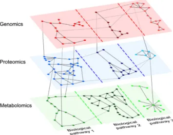
Another example lies in the domain of biology (described further in Section 2.4). One aspect is the type of data, such as genomic, metabolomic or proteomic. Another aspect might be the species, or different biological pathways, as illustrated in Figure 2. If the bio-logical data contains time information, that may also be considered an aspect. While multiple aspects are a possibility for multilayer network data sets, it is not a requirement. A multilayer data set may be defined by a single aspect, which categorizes multiple layers. See Table 1 for a sample list of aspects and layers extracted from the literature surveyed as part of this report. Kivel¨aet al. [KAB*14] provide further examples in their extensive list of multiplex data sets and their associated layers.

Incidentally, Wehmuthet al. [WFZ16] propose an alternative definition they call MultiAspect graphs where they formally define what can be considered as an aspect. Unsurprisingly, they also form a network where nodes are defined using Cartesian products col-lecting multiple values into a single entity. The authors describe MultiAspect graphs as forming a generalization of Kivel¨aet al.’s

Figure 2: A purely illustrative example of multilayer data in the context of biology. The layer can be described by the type of data as a first aspect (genomic, proteomic or metabolomic), and biological pathway being represented as second aspect.

multilayer network. Reconciling these different approaches is be-yond the scope of this paper. Well-developed examples are certainly needed to uncover the full applicative potential of MultiAspect graphs.

2.3. Related graph models

Below, we review related graph models (see also Figure 3) and their differences or resemblances to multilayer networks.

2.3.1. N-partite graphs

Recall that a bipartite graph is made up of two disjoint sets of vertices so that no two vertices belonging to the same set are con-nected. Bipartite graphs can be considered as a case of multilayer networks with two layers and only inter-layer edges. The two mode (i.e. node type) nature of bipartite graphs result in analytics that are different to those of single-mode graphs [BE97]. Bipartite graph concepts are sometimes extended into n-partite graphs, as seen in our example in Figure 3(a), although, in practice, many of the tw-mode restrictions associated with bipartite graph are not fully retained. In practice, systems which model bipartite cases and ex-tensions of bipartite cases, such as the multimodal networks of Ghaniet al. [GKL*13] and the academic network analysed by Shi

et al. [SLT*14], can be considered instances of multilayer net-works. In this case, the authors also make use of bipartite analytics (e.g. adapted centrality metrics) to better understand their network structure.

Bipartite networks can be reduced to single-mode networks via projection on a mode. Such an operation may also be used to define a layer in a multilayer network, if the projection results in a layer that reflects the reality of the system being modelled.

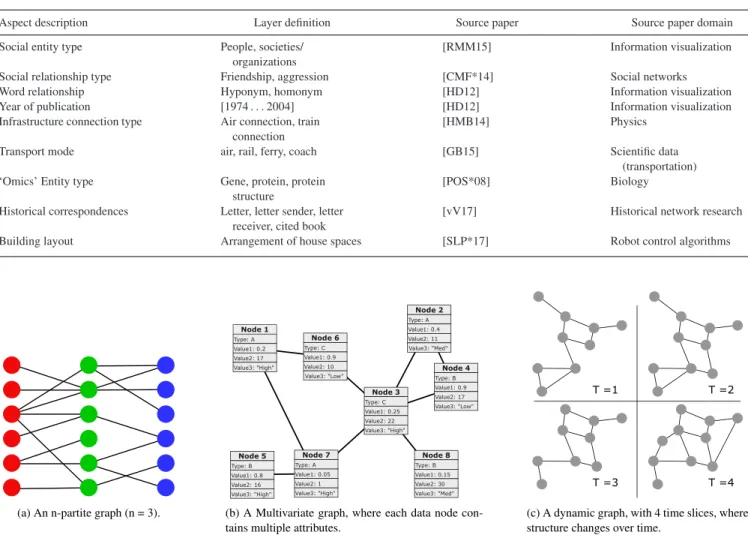
Table 1: Examples of aspects and layers, extracted from papers covered by this survey.

Aspect description Layer definition Source paper Source paper domain

Social entity type People, societies/ organizations

[RMM15] Information visualization

Social relationship type Friendship, aggression [CMF*14] Social networks

Word relationship Hyponym, homonym [HD12] Information visualization

Year of publication [1974 . . . 2004] [HD12] Information visualization

Infrastructure connection type Air connection, train connection

[HMB14] Physics

Transport mode air, rail, ferry, coach [GB15] Scientific data

(transportation) ‘Omics’ Entity type Gene, protein, protein

structure

[POS*08] Biology

Historical correspondences Letter, letter sender, letter receiver, cited book

[vV17] Historical network research

Building layout Arrangement of house spaces [SLP*17] Robot control algorithms

Figure 3: Illustrative examples of related graph models: Each of the three node types (indicated by colour) of the n-partite graph could define a layer within a multilayer network, in this case, all edges would be between layers. For a multivariate graph, node attributes could be used to divide the network into layers. Defining layers by node type in this example would result in three layers, although that may not make sense for the system being modelled, as there would be no edges within the layers of nodes of types B and C. For a dynamic graph characterized by time slices, each time slice can be intuitively understood as a layer. Further insight could be gained by the use of an additional aspect to define layers.

2.3.2. Multivariate graphs

Multivariate graphs [KPW14] are those in which nodes or edges carry attributes or properties. As described by Schreiber et al.

[SKB*14], there is a relationship between multivariate graphs and multilayer graphs. Some variables or attributes in a multi-variate data set often serve the purpose of distinguishing nodes and edges that belong to different layers, e.g. the type of so-cial network platform in our initial example. There are also mul-tivariate visualization applications such as that of Pretorius and van Wijk [PVW08], which define their graph as having dis-crete sets, which can be considered analogous to defining lay-ers. However, in the majority of cases, research into multivari-ate visualization lacks the a priori definition of a layer defined by a physical or conceptual reality related to the system being modelled.

In faceted data sets, multivariate data items are grouped in multi-ple orthogonal categories. Originally used as an approach to search and browse large data stores and text corpora [SCM*06, CSL*10], later work extended the faceted approach to include relationship vi-sualization [LSR*09, ZCCB13]. Data sets can have many different facets such as spatial and temporal frames of reference, or multiple values per data item and as such can be considered multi-faceted. Visualizations for multifaceted data are those which show more than one of these facets simultaneously (see Hadlaket al. [HSS15] for a survey of multifaceted graph visualization techniques). Hadlak

et al.discuss primarily four common facets of network structure considered in network visualization, and their composition: parti-tions, attributes, time and space. These facets may be considered to be very similar to instances of Kivel¨a et al.’s aspects. How-ever, they can be considered as different ways of exploring a sin-gle data set (which is unsurprising given the origins of a faceted

visualization). The techniques described are still very useful for de-veloping approaches for visualizing layers, particularly where the layer type matches the Hadlaket al.’s selected faceted categories. However, faceted network visualization approaches do not meet all the needs for multilayer network visualization. While multilayer networks may use notions similar to these facets to characterize layers, multilayer network visualization also focuses on the inter-actions between layers and the role of layers in the network as a whole.

2.3.3. Dynamic graphs

Dynamic graphs are graphs whose structure (nodes and edges) and/or associated attributes may change over time. Analysts are often interested in comparing the state of the network at different points in time. Within the domain of complex networks, Boccaletti

et al. [BBC*14] consider the dynamics of multilayer networks, and in many cases, time slices of a dynamic (or temporal) network are simply mapped to layers. The notion of dynamic networks is also mentioned by Kivel¨aet al., who note that they can be considered as a type of multilayer network. A set of dynamic time slices can be considered layers in an aspect representing time. As multilayer networks can have multiple aspects, a temporal aspect might be just one of many. In their report on dynamic network visualization Moodyet al.[MMBd05] explain the importance of ‘multiplicity’ in social networks, i.e. the overlap of types of relations. In particular, they point out that linking relational timing to tie types allows better investigation of social dynamics. A recent survey of dynamics graph visualization techniques was provided by Becket al. [BBDW17], but does not consider layers in any context other than a hierarchi-cal graph.

2.4. Application domains and data

Across all of the application domains mentioned in Section 1, ad-vances in sensors, scientific equipment and technology mean that researchers have access to more data than ever. This wealth of com-plex data is often best understood as a multilayer network model.

2.4.1. Life sciences

Within biological network visualization, there are many con-texts in which a multilayer network approach may be benefi-cial [GMD*18]. Biologists have access to more genomic, proteomic and metabolomic data, allowing for the construction of complex multilayer models of intricate biological processes. Interactions tak-ing place within the genomic, proteomic and metabolomic levels can be modelled as individual networks, but interactions also occur between elements sitting in different omics levels within a larger biological system, where the aspect characterizing the layer is the node type [CWV*10]. This corresponds to the strongly rising topic of systems/integrative biology, where the challenge consists in un-derstanding the interplay and the cascade of effects taking place at the different levels of the biological system at hand [GOB*10, KTT13]. A prominent task for biologists analysing biological path-ways consists in comparing a species-specific pathway to a refer-ence pathway [MMF17]; in this specific case, species type can be

considered a defining aspect for a layer. Another task is to com-pare tissue-specific interaction networks to understand why certain tissues, e.g. plant root tissues, synthesize certain molecules which are not found in other plant tissues. In this case, tissue type is the defining aspect for a layer.

2.4.2. Social sciences

Data sets within Social Network analysis frequently contain mul-tiple types of edges (to support examining the different types of relationships between people, e.g. more recently [CMF*14], but also in much earlier work such as [BS85, LP99]), or multiple types (or modes) of nodes, e.g. modelling a citation network containing researchers, institutions and publications [GKL*13]. Within social sciences, there are also contexts in which many networks may be compared to one another. For example, examining social networks produced as a result of cell phone activity, as done by Freireet al.

[FPSG10]. The contemporary use of multiple online social networks provides a vast amount of data. This allows for complex social mul-tilayer networks to be built, which may help sociologists gain deeper insight [RMV14].

Other fields such as food microbiology have adopted Social Net-work Analysis techniques, and applied them to understand problems such as the spread of disease. This can be seen in the work of Crabb

et al. [CAD*17] to understand the spread of salmonella in a large poultry farming enterprise. Different networks are generated based on contact between different types of entities. From a multilayer perspective, contact between entities can be considered an aspect, with the entity types defining the different layers.

2.4.3. Digital humanities

Within digital humanities fields, such as digital cultural heritage, ar-chaeology and data journalism, many multilayer approaches [vV17, MDG16, DHRL*12, SGo16, RRV*18, MBvL*17] can be found. Digital access to source texts and natural language processing tech-niques such as Named-Entity Recognition and Topic Modelling allow for vast Digital Humanities data sets to be built [MDG16]. Co-occurrence relationships between people names, locations, orga-nizations as well as other entities form a typical multilayer network whose analysis may reveal insightful interaction patterns.

2.4.4. Infrastructure

Modern vehicles often provide a wealth of information about mod-ern transportation networks. These networks can also be modelled as multilayer networks. For example, Haluet al. [HMB14] model the air and rail transportation networks of India as layers in a multilayer network. A paper by Gallotti and Barthelemy [GB15] is another nice example. The Internet and associated infrastructure provide vast amounts of data about themselves and can be modelled as mul-tilayer networks, as done by Reiset al. [RHB*14], who represent the power grid and the Internet as separate interdependent layers in a multilayer infrastructure network. Recent work concerning Urban Infrastructure Systems highlights the necessity to adopt an inte-grated approach to urban planning taking into account the interplay between multiple networks such as transportation networks, energy

networks, telecommunication networks and water/wastewater net-works [Der17]. Some of the related objectives may be to reduce the cascading of failures across these networks [BPP*10], but also to develop an efficient repair strategy to restore services after dis-aster [SDH16]. The precise representation of buildings to support robot control algorithms is a related domain as seen in [SLP*17]. In this work, the graph represents a layout of the floors of the building with their interconnections. A layer is a floor containing rooms. An edge represents a direct connection between two rooms. Interlayer connections modelled connections between floors. This kind of model reduces the amount of data to be analysed by a robot. The vast number of instances of complex data sets produced across all these domains demands a visual approach to help under-stand it, and that approach will often be multilayer network visual-ization.

2.5. Complexity and human performance

Multilayer networks are implicitly more complex than standard net-works, which is not surprising given their origins in the domain of complex systems. The complexity can be increased by the type of task, the sheer volume of data or the density of its connectiv-ity. Within information visualization, there have been many studies completed examining the impact of these various types of complex-ity on human performance at specific tasks. For example, Ghoniem

et al. [GFC05] examine the impact of edge density on choice of visualization approach, see Section 4.3.3. The notion of practi-cal densities for empiripracti-cal evaluation is one which prompts much discussion [Mel06]. While graph size has been recognized as an important factor for quite sometime, there is no widely accepted definition of what is a large or small graph [vLKS*11], with many empirical evaluations running pilot studies or basing their chosen size of large graph on assumptions rather than a standardized defi-nition. While we do report on the state of empirical evaluations with respect to multilayer networks (see Section 4.6), the topic of human performance and network complexity is a vast topic in and of itself; therefore, a full analysis is beyond the scope of this state-of-the-art report on multilayer networks. For a detailed survey on network complexity and empirical evaluations, the reader is referred to the work of Yoghourdjianet al. [YAD*18].

3. Methodology Followed

This section is about the structure of the survey which is built on a categorisation of the important features of multilayer network and how we selected papers cited in the many domains we cover.

3.1. Categorization

The categorization of the most important features of multilayer network visualization that are to be considered for each paper is built in a manner consistent with Munzner’s nested visualization design process model [Mun09]:

Tasks and analysis. Multilayer systems that address new prob-lems and domains may expose tasks that do not fit in existing task taxonomies, such as [LPP*06, PPS14]. New analytics have been

developed for multilayer networks, and new visualizations have been developed as a result, e.g. [DDPA15].

Data definition. This aspect of the review looks at the nomen-clature used for the data set e.g. multiplex, heterogeneous, which aspects are used to define layers across the data, as well as the structure of the data.

Visualization approach. We analyse and categorize the various visualization approaches described, identifying novel approaches and novel applications of existing approaches, e.g. [BISP16]. While many visualization systems described in this survey were not ex-plicitly identified in the original source as being for multilayer net-works, we point out ways in which they may be applicable and targeted to them.

Interaction approach. Interaction with multiple layers will of-ten be more complex and requires innovative techniques, such as [HD12, SLT*14, RMM15].

Attribute visualization. Multilayer networks can also carry mul-tivariate data [SKB*14, DHRL*12]. Under this category, we will examine the impact of multilayer structure on attribute visualization.

Empirical evaluation. Empirical evaluation is a challenge for in-formation visualization [Pla04]. Within the domain, there are many guides to evaluation such as [Pur12]. However, techniques devel-oped in application domains may not have been exposed to the same level of rigour as those developed within the visualization domain. It is important to understand which novel techniques have been empirically validated with respect to their usability.

3.2. Papers selection

The wide range of application domains makes performing a com-plete survey highly challenging. Within the domain of visualization, we queried prominent journals and conferences for a list of keywords related to multilayer networks. Our main search engines wereIEEE Exploreand theACM Digital Library. The list included the terms (and variants of the terms using hyphens) multilayer, multilevel, faceted, multirelational, multimodal, multiplex, heterogeneous and multidimensional. The ambiguity of some of these terms meant that some completely unrelated papers were returned. These were removed from the list based on their abstract. The prominent vi-sualization venues includedIEEE TVCG(and implicitlyVASTand

Infovis),CHI(includingSIGCHIandTOCHI),Computer Graphics Forum(and implicitlyEurovis),Advanced Visual Interfaces, Paci-ficVis,Graph Drawing and Network Visualization(formerlyGraph Drawing) and the journalInformation Visualization.

Due to the wide range of application domains and numerous publication venues in each, it was not feasible to perform such a formalized search within them. We used our initial list of visualiza-tion papers, as a seed adding papers from the applicavisualiza-tion domains which were cited by or cited them as found using Google scholar search.

Additional papers were also added to the list of those reviewed based on feedback from reviewers of this STAR, if they indicated that the papers would be valuable additions. Each paper was re-viewed by at least one co-author, and the review shared with all other authors using a wiki. Papers were summarized based on the characteristics described in Section 3.1. Reviews of the paper were discussed at group meetings between the co-authors to provide a final decision on which papers should be included or excluded. All final text describing the papers within this work was validated by all co-authors.

As stated in Section 1, the goal of this survey is to rec-oncile the many visualization approaches from the information visualization field and the application domains. Many techniques have been extracted from papers which may not have focused explicitly on multilayer techniques, perhaps using one of the names described in Section 1, e.g. heterogeneous. However, the techniques are included as we believe that they are of inter-est to researchers who wish to visualize multilayer networks. As part of the review process, some papers were considered, based upon the keyword search described above; however, they were omitted from the final state-of-the-art report due to their con-tent not being related enough to the visualization of multilayer networks.

4. Survey of Multilayer Graph Visualizations

In this section, we begin by defining and illustrating a task tax-onomy for multilayer graphs. Consistent with Munzner’s model, we survey various data definitions on which the visualizations pre-sented hereafter are built, as well as relevant interaction techniques. The survey encompasses the visualization of attributes in the con-text of multilayer networks and closes with considerations about visualization evaluation.

4.1. Tasks and analysis

Numerous literature surveys [LPP*06, APS13, PPS14, KKC15, BBDW17] list tasks relevant to the visual analysis of different types of networks (general, evolving, multivariate, etc.) and tasks have been proposed on a domain specific basis, e.g. [MMF17].

Leeet al. [LPP*06] provide a general graph task taxonomy. At its top level, it considers Topology Based Tasks, Attribute Based Tasks,Browsing TasksandOverview Tasks. It explicitly specifies that the high-level tasks of comparison of graphs and identifying graph change over time are not covered by the taxonomy.

Pretoriuset al. [PPS14] focus on multivariate networks. The highest level of their taxonomy divides tasks as follows:Structure Based Tasks,Attribute Based Tasks,Browsing TasksandEstimation Tasks. The categoryEstimation Tasksis further subdivided and more detailed than Leeet al.’sOverview Tasks. The name was chosen to capture that these tasks are not easily definable using lower level tasks and are considered more high level, and are not focused on giving precise answers. Within this categorization, there is a com-parison task, which may be of some relevance for multilayer graphs. It covers comparing information at different stages of a networks

development, and determining causation, i.e. providing an expla-nation for the differences between two snapshots of a changing network.

While Pretoriuset al.do consider graph change as part of their multivariate tasks taxonomy, the taxonomies of Kerracher et al.

[KKC15] and Ahnet al. [APS13] both focus specifically on dy-namic networks, also known as evolving or temporal networks. At the highest level, Ahnet al.’s taxonomy focuses on three groupings:

Entities,PropertiesandTemporal Features. The temporal features are grouped as Individual Events, the Shape of Change and the

Rate of Change. These are considered from the individual entity level to the entire network level, and for both structural and domain properties. Kerracheret al.’s taxonomy builds on the non-network specific taxonomy of Adrienko and Adrienko [AA06] by extending it to include network data. It considers both elementary and syn-optic tasks, as defined by Andrienko and Andrienko (elementary tasks involve individual items and characteristics, synoptic involve sets of items considered as an entity), but further divides synoptic tasks into three categories. These are tasks considering graph sub-sets, tasks considering temporal subsets and tasks considering both graph and temporal subsets. The taxonomy differs from Ahnet al.’s in that it focuses more on the tasks that data items take part in, rather than the data items themselves, and considers a more general con-cept of pattern changes that captures relational changes in the net-work, as well as considering tasks which provide context for graph evolution.

Murrayet al. [MMF17] propose a taxonomy in the context of bi-ological pathway visualization that contains tasks concerning com-parison, attribute analysis and annotation that relate to multilayer networks. Although most task taxonomies that have been developed so far do not directly address multilayer networksper se, they could be further adapted or extended to target multilayer network visu-alization. Existing literature does mention specific tasks that may be relevant for multilayer network visualizations, which we cover in this section. Some tasks may involve the temporal dimension as well (such as tracking the evolution of nodes or edges at different moments).

Unsurprisingly, tasks that are specific to multilayer networks re-volve around the notion of a layer. Tasks often boil down to ma-nipulating elements within one layer, or across several layers, or manipulate the layers themselves. These manipulations often lead to lower level tasks, which are also critical for visual analytics tasks (identifying actor roles, grasping group interaction or communica-tion patterns in social networks, etc.).

In the survey work of Pretoriuset al. [PPS14], a task is schema-tized as a process:

Select entity→Select property→Perform analytic activity

We see here an important difference with the process of perform-ing a task on a multilayer network involvperform-ing layers. Conceptually speaking, layers are genuine building blocks of a multilayer net-work. They are neither a simple (sub-)network nor a mere property of a node or edge. They are a conceptual construct that fully enters the analytic process when performing a task (involving the multi-layer nature of the network).

We report here on different approaches or systems that support tasks relevant to multilayer networks. In many cases, authors have not explicitly expressed tasks in terms of layers, but rather refer-ring to properties of the data they consider. This is the case for authors considering tasks related to group comparison or reconfigu-ration [HD12, CLLT15]. To this end, in anticipation of Section 5.1, we propose task categories specific to multilayer networks. We tar-get tasks directly involving visualization, as opposed to tasks that can be addressed through computational means only.

Task category A—Cross-layer entity connectivity (e.g. inter-layer path). Tasks in this category aim at exploring and/or inspecting connectivity involv-ing paths traversinvolv-ing multiple layers. Understandinvolv-ing how shortest paths expand across layers, inspecting what nodes do occur on these paths are typical examples of tasks in this category. Being able to explore cross-layer connectivity has been identified as an important user task in [GKL*13]. Associative browsing in Refinery [KRD*15] is a good illustration of cross-layer connectivity task. It performs cross-layer random walks and collects nodes from different layers in a single view. The leapfrogging operation in Detangler [RMM15] is another good illustration of cross-layer connectivity building a dual view reflecting how/what layers get involved when hopping from node to node (see Section 4.4).

Task category B—Cross-layer entity comparison. Tasks in this category aim at comparing entities (typically, nodes) across different layers; this re-quires the ability to query entities across layers. The task may con-cern the same (set of) node(s) over several layers; or distinct nodes that are somehow linked across different layers. Jigsaw [SGL08] typically supports this tasks by allowing users to identify entities (persons, places, etc.) through several documents (seen as layers in a multilayer document network). FacetAtlas’ [CSL*10] multi-facet query box is another good example.

Task category C—Layer manipu-lation, reconfiguration (split, merge, clone, project). Tasks in this category aim at manipulating the layer structure itself. Such manipulation may allow for previously unseen relation-ships and structure to be revealed, and allow for new perspectives on the underlying data. Combining layers through drag and drop operations, as in the work of Hasco¨et and Dragicevic [HD12], is a perfect illustration of this type of task; another example is g-Miner [CLLT15] which allows to create, edit or refine the grouping of elements.

Task category D1—Layer compar-ison based on numerical attributes. Tasks in this category support com-paring layers to one another based on numerical measures summarizing layer content and structure. Typically, layers could be compared by looking at how node degree distributions compare layer-wise. OntoVis [SMER06] (where layers map to node type) sup-ports layer comparison tasks using a metric they call (inter-layer) node disparity. Pretoriuset al. [PVW08] propose a quite

elaborate approach and system to perform multi-attribute-based layer comparison.

Task category D2—Layer comparison based on topological, connectivity pat-terns.Tasks in this category support com-paring layers through non-numerical but rather topological features of layers (e.g. group structure). A layer could be hierarchical (inher-itance), while another could show a strong scale-free structure, for instance. The work by Vehlowet al.[VBAW15] is a typical tech-nique allowing to compare group structure across layers. Tasks R5 and R12 in GraphDice [BCD*10] are another good illustration of such tasks. In the biological domain, the toolNetaligner[PCA12] compares different biological networks, which can be considered analogous to layers, and visualizes them in a single visualization to allow a user to determine how well the networks are aligned, i.e. overlapping in terms of nodes and edges.

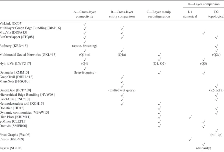
Table 2 summarizes task categories supported by a selection of systems and techniques cited and described in this report. 4.2. Data definition

This subsection looks at the various data definitions found in the visualization literature on which visual representations of networks with multilayer characteristics are built. Only a few approaches explicitly mention the use of multilayer networks (both as data underlying the visualization and as a visual encoding). Most systems dealing with multivariate networks couple relational data with node and edge attributes [SMER06, Wat06, BCD*10, HP14] often using table-based representations [KS14, HP14]; they do not consider any data or attribute specifying a layer structure. Caoet al. [CSL*10] considerclassesof entities they call ‘facet” which appear to naturally map to layers of nodes (see Section 2.3.2). Among all, the work of Pretoriuset al. [PVW08] is a notable exception as it introduces the notion of layers without using the term, and explicitly defines nodes as Cartesian products of attributes (see Section 2.1).

Other systems and approaches infer multilayer structure by ag-gregating data from multiple sources, whether databases [KSW14] or a collection of ego networks (as in [DACP15]) and/or personal data [HTA*15]. Interestingly enough, some systems do not directly target the visualization of multilayer networks, but use multiplex and/or hypergraph representations to build query graphs or summa-rize query responses [TS13, SW13].

Obviously, MuxViz [DDPA15] relies on the exact definition and implementation (see Section 2.1) introduced by [KAB*14], which is also the case of authors mentioning explicit use of the MuxViz framework [GB15]. Elementary layers originating from aspects of the network, such as time or node/edge type, are quite similar to the facets described in [HSS15]. Detangler [RMM15] relies on an explicit encoding of layers, with a goal to allow an easy exploration of inter-layer correlation (see Section 4.1). Making a distinction between layers as being either structural or functional (or of any other type) may be useful depending on the pursued goal [ATSN17]. 4.3. Visualization approaches

From a multilayer network perspective, previous work in network visualization techniques may be classified based on their awareness

Table 2: A selection of techniques/systems grouped as far as possible by task categories, relevant to multilayer networks, that they either implicitly or explicitly support. Notes in parentheses refer to task labelling/naming as indicated by authors in their paper.

D—Layer comparison

A—Cross-layer B—Cross-layer C—Layer manip. D1 D2

connectivity entity comparison reconfiguration numerical topological

VisLink [CC07] √

Multilayer Graph Edge Bundling [BISP16] √ √

MuxViz [DDPA15] √ √ √

BicOverlapper [STQ08] √ √ √

√

Refinery [KRD*15] (assoc. browsing)_{√ √} √_√

Multimodal Social Networks [GKL*13] (Q1b,c)_√ (Q1a) √_{√ √} (Q2c)

HybridVis [LWYZ17] (Q4)_√ (Q1, Q2) (Q3)

Detangler [RMM15] (leap-frogging) √ √

GraphTrail [DHRL*12] √

ManyNets [FPSG10] √

√ √

GraphDice [BCD*10] (multi-facet query) (R5, R12)

Hierarchical Edge Bundling [HVW08] √ √

FacetAtlas [CSL*10] √ √

NetworkAnalyst tool [XGH15] √ √

Donatien [HD12] √ √

Dynamic communities [VBAW15] √ √

Hive Plots [KBJM11] √ √

g-Miner [CLLT15] √ √

Ontovis [SMER06] √ √ _√

Pivot Graphs [Wat06] (roll-up)

Circos [KSB*09] √ _√

Jigsaw [SGL08] (disparity)

of the notion of a layer. When this is the case, layers are visu-ally encoded using any appropriate Gestalt principle in a way that structures the spatial representation; they are also manipulated as visual objects in their own right as detailed in Section 4.1. This is why this section is organized based on the type of visual encoding used to show layers explicitly. This survey also documents and re-flects on the widespread use of weaker visual cues (in the sense of Mackinlay’s ranking of perceptual tasks [Mac86]) to encode layer information, such as node or link colour.

4.3.1. One-dimensional representations of layers

Existing visualization techniques use a large variety of one-dimensional (1D) representations of layers (see Figure 4 for ex-amples of basic 1D visualization). This type of visual encoding relies on the law of continuationof Gestalt theory, such that the eye may perceive paths on which nodes are arranged whether these paths are actually drawn or not. This applies to circular paths, as well as straight axes, or any curve shape.

Circular representations. This body of work includes concentric circles, where each circle stands for a layer. Concentric circles are

Figure 4: A simple illustrative example of a vertical-axis-based one-dimensional layout and a circular layout. In both cases, it is the ordering of the nodes that is more important than coordinate position.

used in [BSH13] where the focus is on depicting paths through the whole set of layers (Task categoryAin our taxonomy). Node order optimization and edge bundling are used to reduce edge clutter. A similar layout is used in the ring view of MuxViz [DDPA15] but focuses on visual correlation analysis of node attributes across

different layers (Task categoryD1). Node colour encodes attribute values (see Section 4.5 and Figure 16), while ring order and ring thickness encode computed layer-level metrics. Similarly, Circos [KSB*09] is a popular tool for comparative analysis of genomic data, where each ring/layer may stand for a biological sample. To compare node attribute values across samples, a histogram is wrapped around each ring (Task categoryD1).

Chord diagrams display layers as arcs composing one overall cir-cle. They are used in the NetworkAnalyst tool [XGH15] to analyse gene expression data. Links between layers are drawn as splines connecting identical nodes occurring in different layers/arcs (Task categoryB). The analyst may click on a pair of arcs to highlight their common nodes (and the bridging links). A similar approach is followed in [AAMH13, CMF*14]. In the presence of multilevel cat-egorical attributes as in [HEAE16], each arc of the chord diagram can further be split hierarchically (Task categoryC). The chords would then connect nodes at the leaf level across all layers where they are repeated.

Axis-based node-link representations. In this category, a layer is materialized by a straight 1D axis. Obviously, the representation of a multilayer network lays out nodes on several such parallel axes. An important way of distinguishing axis-based visualizations re-lates to the type of variable represented by the axis, whether it is quantitative, e.g. a graph metric like node degree or any numeric node attribute, or ordinal/ranking-based. Despite the visual simi-larity to the Parallel Coordinates plot [ID90], a polyline represents a path between nodes sitting in different layers/axes, rather than a thread linking attribute values across different columns in a given table entry. Crnovrsaninet al.[CMF*14] describe a view that uses such parallel axes arrangement, and alternatively chord diagrams. An example of analyses they run consists in comparing the ‘ag-gression network’ among students in four different schools, based on student race group. They show that smaller groups do not show internal aggression patterns, while larger groups victimize every-body equally (within the same group and in other groups). In this case, the analyst is more interested by topological considerations at the group level, and structural differences between layers (Task categoryD2).

Ghaniet al.[GKL*13] provided an approach called parallel node link bands (PNLBs). Nodes are positioned uniformly across spaced parallel axes which represent layers defined by the node type (or mode), see Figure 5. Edges are only drawn between adjacent layers, and within layer, edges are shown in a separate visualization. Node order on axes can be set based on edge attributes or connectivity to other layers. They use their approach to analyse the National Science Foundation (NSF) funding data set. Examples of tasks they carry out include determining whether some NSF programme managers award funding to some Principal Investigators (PIs) more often than others on a three-layer networking containing programme managers, projects and PIs. This is an instance of Task categoryAwhere the focus is on paths traversing all layers.

The list view of Jigsaw [SGL08] provides an overview of entities grouped by type, with edges being drawn between connected entities in adjacent lists. One of the main utilities of this system is to relate different types of named entities (people, geographic locations and

Figure 5: The parallel node-link bands (PNLBs) representation of [GKL*13]. Each axis is a distinct set of vertices. Edges are only displayed between adjacent axes. Some axes show a quantitative value, e.g. project budget, while others display text strings, sorted based on a graph metric or alphabetically.

Figure 6: The hive plot representation of health data by [YTL*16] showing four layers/axes: toxicity type (duplicated), material and particle size. Edges are only displayed between adjacent axes. The vertices on the horizontal axis are coloured based on their cluster membership.

organizations) mentioned in the same documents. Entities which are connected to a currently selected item are highlighted by colour across all lists. It therefore emphasizes the analysis of paths across all available layers (Task categoryA). The list view is complemented by a node-link and a matrix-like scatterplot view, among others.

Hive Plots [KBJM11] differ from the previous techniques in that they arrange the axes radially. Originally introduced for the anal-ysis of genomic data, they have been used in other domains like performance tuning in distributed computing [EW12] and in the domain of health [YTL*16], as can be seen in Figure 6. In [KBJM11], node (gene) subsets are placed on separate axes based on a node-partitioning algorithm. The fundamental questions they answer using hive plots include determining differences in connec-tivity patterns between layers (Task category D1). An element’s position along its axis is often calculated based on a graph metric, e.g. node degree in [EW12] and may be based on the raw or normal-ized value of an attribute. Edges are displayed between adjacent axes only. Yet, visual clutter may still occur with real application data. Layer duplication as in Figure 6 is convenient when the relationship to a non-adjacent axis becomes necessary (Task categoryC).

Figure 7: A simple illustrative example of 2D, 2.5D and 3D visu-alizations of a network. The 2D layout (left) is a standard node link layout where nodes are positioned withxandycoordinates and, usually, an orthogonal projection is used to render the visualization. The 2.5D approach (centre) draws sets of nodes on 2D planes at different depths. For the 3D example (right), nodes are at different depths in that they actually have an individualzcoordinate (depth value) for position. In this example, the nodes themselves are 3D objects (spheres) rather than circles, and are shaded to clarify their 3D shape. 3D network visualizations are usually rendered with a 3D projection. As can be seen from this figure, depth is difficult to convey in a static 2D image. 3D visualizations usually require some level of camera movement to reveal occluded data, as well as the depth aspect to be conveyed through motion and/or stereoscopy.

4.3.2. 2D, 2.5D and 3D node-link representations

Across the various papers we surveyed, node-link layouts cropped up frequently. As illustrated in Figure 7, for the standard two-dimensional (2D) layout,xandycoordinates are assigned for each node. For the 2.5D approach, sets of nodes are assigned to planes at a different depth, and for the three-dimensional (3D) approach, the nodes are usually assigned a different individual depth (z coordi-nate). The MuxViz toolkit[DDPA15], from the domain of complex systems, utilizes several variants of node-link visualizations. They are also used in other domains that depend on complex systems theory [GB15, BBB*16, DD17].

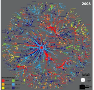
A widespread visual design consists in encoding layer informa-tion using node colour or shape, as depicted in [MMBd05, FHK*09, KSW14, ZB16]. Colour coding of edges is also used in [Duc17, DDPA15]. This design choice relies on the law of similarity of Gestalt theory (colour similarity in this case). This design is often adopted when the multivariate nature of the network is the driving motivation of the visual design. For instance, Figure 8 represents flows of maritime traffic using colour to encode different modes of shipping (or layers). The analyst looks among other things at structural changes over time, where different layers encode dif-ferent time slices (Task categoryD2). But if the analyst is inter-ested in analysing a given time slice, different layers may represent different shipping modes. The related task consists of comparing structural differences among the different modes. In similar visual designs, layer information is diffuse, relationships between lay-ers and within the same layer are mixed and uslay-ers seldom get a handle on layers to manipulate them directly. Nodes belonging to different layers are intertwined in the 2D plane, when standard node-link layouts are used, and edge clutter is problematic. Layer-related tasks may therefore be difficult to carry out under these circumstances.

Figure 8: A multilayer network visualization describing the flow of maritime traffic. Nodes represent ports and different edge colours represent different modes of shipping, taken from [Duc17].

While not explicitly designed with multilayer network visual-ization in mind, constraint-based layouts offer the possibility to constrain a 2D node-link layout in such a way that respects the con-cept of layers. For example, theSetColaconstraint-based layout of Hoffswellet al. [HBH18] allows users to apply layout constraints to sets of nodes, which might easily correspond to layers. Such a layout approach supports analysing cross-layer connectivity (Task categoryA) as well as layer comparison (Task categoryD2). The examples covered by the authors include a food web networks and a network modelling a biological cell, and both of these data sets can be considered to have multilayer characteristics. The multilevel layout approach ofTopolayout[AMA07] is also not designed with multilayer networks in mind, but, as an approach, may be of inter-est in the multilayer case. Topolayout is a feature-based approach that decomposes an graph into a hierarchy of features (hence, being considered a multilevel algorithm) and chooses a suitable algorithm to layout each feature. Within a multilayer network, the structure of each layer may be very different, requiring an approach that can adapt to the different features in each. The highest level feature detected by the Topolayout algorithm is a connected component; therefore, the algorithm could be adapted to consider each layer as a connected component, but also would need to be enhanced further to consider the impact of inter-layer connectivity.

Inspired by the multilevel nature of some problem areas, e.g. bi-ological networks, the 2.5D approach materializes layers as 2D translucent parallel planes in a 3D layout, similar in spirit to Figure 2. This visual design relies on the law of uniform con-nectedness of Gestalt theory. It separates links lying within layer from those between layers providing a more natural support for path-related tasks (Task categoriesAand B) than traditional 2D node-link layouts, but 3D navigation is required to allow the user to change his perspective on the data and resolve visual occlusion

problems. As opposed to 1D axis-based representations, the par-allel 2D planes provide space to lay out intra-layer links. In the 2.5D category, some approaches use colour redundantly to encode layer information as in [FHK*09]. Other visual design options for 2.5D consist in using colour to encode an attribute value or a com-puted metric, e.g. community assignment by a community detection algorithm as in [DDPA15], across the different layers. From the bi-ological domain, theArena3Dapplication visualizes biological data using an interactive 3D layout, where layers are also projected onto planes, and entities are connected across layers by edges rendered as 3D tubes. The authors demonstrate its effectiveness by analysing the relationship across layers, based on proteins and genes associated with a specific disease (Task categoryA).

The use of 3D layouts is much less common in the information visualization research community. While some work has shown that there may be some benefit to 3D layouts, this is only under stereo-scopic viewing conditions [WM08]. Outside of stereostereo-scopic view-ing conditions, there are no empirical studies which demonstrate usability gains from a 3D graph visualization [GPK12].

A more widely accepted approach in information visualization, especially for the purpose of comparative analysis of graphs, con-sists in using small multiple views. This is often used for graph matching tasks, where the focus is on understanding commonali-ties and differences between a set of related networks [HD12]. In the context of this paper, the networks that need to be matched are distinct layers in a larger multilayer network (Task categoriesD1 andD2). Whether in a 2.5D setting or in a flat small multiples set-ting, one challenge consists in ensuring that duplicate nodes are laid out consistently across layers, by introducing constrained layout strategies as in [FHK*09, HD12] to better support cross-layer entity comparison (Task categoryB). Node-link layouts have been used to compare networks visually, as done by Andrewset al. [AWW09] and Di Giacomoet al.[DGDLP09], but in many situations, other approaches may be more suitable (see Sections 4.3.3 and 4.3.5).

More generally, coordinated multiple views are often used in the domain of information visualization, and in many applications, e.g. the analysis of micro-array data [STQ08]. In this case, 2D node-link views may be used as one of multiple complementary visualizations of a multilayer network, e.g. [KRD*15, GKL*13, SGL08]. It is yet possible to eschew the idea of using a node-link visualization al-together, for example, using aggregate views of nodes (based on attribute data), such as a bar chart enhanced with arcs [DHRL*12]. Coordination between views is common, e.g. brushing and linking. The Detangler [RMM15] application builds on this by also har-monizing layouts between views. It supports several task categories identified in this survey, namely cross-layer connectivity (Task cate-goryA), layer manipulation (Task categoryC) and layer comparison (Task categoriesD1andD2).

Edge visualization. The complex structure of multilayer graphs makes edge visualization an important challenge. It may be impor-tant in some cases to distinguish between inter-layer and intra-layer links, in other cases the number of layers may cause enough clutter with respect to edges, that a visualization becomes less understand-able. In some cases, the chosen solution is to simply not draw all edges and to allow the user to choose which edges to see via

interac-Figure 9: The multilayer edge bundling of [BISP16].

tion to ease inter-layer comparisons (Task categoryB). For example, the PNLBs technique [GKL*13] only draws inter-layer edges be-tween nodes on parallel axes, and intra-layer edges are displayed in a separate visualization. The well-established technique of edge bundling [Hol06] has been adapted for the multilayer use case by Bourquiet al. [BISP16]. The authors bundle all edges in a single visualization, in an aesthetically pleasing manner, with edges being kept adjacent to each other when they share a common path, and edge crossing being avoided (see Figure 9). This approach is useful for showing edges from multiple layers in a single visualization (where there is no division of nodes between layers); the approach is agnostic to the source or target layer, or whether the edges are between or within layer (Task categoriesAandB).

Within their list-based view, Crnovrsaninet al. [CMF*14] use edge bundling between different list columns as a clutter reduction technique clarifies similarities between different edge types. The au-thors essentially group edges based on relation type, by clustering the vertices and altering the clustering based on vertex mode.They also use a modified edge bundling in their circular layout, which distinguishes within-mode edges and between-mode edges, see Figure 10.

Quite naturally, the visualization of edge group structures, as sur-veyed by Vehlowet al. [VBW17], presents a lot of similarities with multilayer network visualization and some work cited (e.g. Detan-gler) can be easily adapted especially for cross layer connectivity and layer reconfiguration (Task categoriesAandC).

4.3.3. Matrix-based visualizations

Standard node-link representations of graphs give equal importance to nodes and links and aim usually to convey structural properties

Figure 10: Edge bundling as utilized by [CMF*14]. Within cate-gory edges are routed around the exterior of the circle. Between category edges are routed via the interior of the circle and bundled.

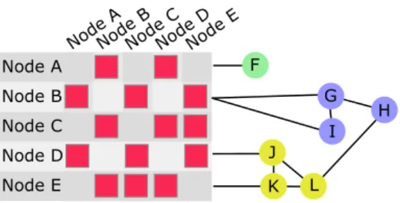
Figure 11: A simple illustrative example of a matrix visualization and the corresponding node-link visualization.

Figure 12: A simple illustrative example of a hybrid approach, mixing both matrix and node link in a single visualization.

of the graph at hand. They may, however, be difficult to read, due to edge clutter, for moderate size graphs, and for the more complex networks encountered in many real usage scenarios. When dealing with large and/or dense graphs, matrix-based representations were found to be more readable than node-link diagrams [GFC05] for many tasks, except path finding. They have also been shown to out-perform node-link visualizations for some tasks concerning clusters

of nodes [OJK18]. Matrix-based visualizations consist of laying out nodes as the rows and columns of a 2-way table. A link between two nodes is often represented as a rectangle at the intersection of the associated row and column, as illustrated in Figure 11. This avoids altogether the edge clutter problem of standard node-link represen-tations. Colour is often used to encode the weight of the links, when link attribute values are available. This makes matrices very similar, if not identical in essence, to heat map views frequently used in biology and other domains [WF09]. Other visual designs include using circles at the intersection of rows and columns with size and colour encoding link attribute values, as in [CMH12]. Matrix repre-sentations have been used to visualize homogeneous graphs (nodes of one type), e.g. in software engineering [VH03], and bipartite (or 2-mode) graphs, e.g. in software performance tuning [GCFJ05]. In the latter work by Ghoniemet al., the analyst needed to compare the graph structure and edge weight distribution before/after a software revision by contrasting the corresponding matrix representations, and also to monitor the runtime behaviour of the software through the animation of the matrix representation as the graph structure and edge weights changed over time.

The ability to detect link patterns in a matrix view is conditioned by the use of an appropriate ordering of rows and columns. Various seriation algorithms [Che02, Lii10, Fek15] reorder the rows and columns of the matrix to create dense rectangular blocks of links. Community detection in a bipartite graph consists in finding groups of nodes in one layer which are densely connected to groups of nodes found in the second layer (Task categoryA). Two-way hierarchical clustering is commonly used with biological data for this purpose. The BicOverlapper system [STQ08] uses bi-clustering methods to find such relationships between groups of genes and related groups of medical conditions. On the visual side, BicOverlapper uses coor-dinated multiple views, one of which employs convex hulls within a standard node-link representation to materialize groups of genes, akin to the notion of elementary layers described in Section 4.2. The overlapping convex hulls are meant to support the identification of commonalities and differences between layers (Task categoriesB andD2).

In the presence of multiple layers, the comparison of link patterns between many pairs of layers may be useful to the analyst (Task cat-egoryA). Laying out small multiples of matrix views side by side is one approach. Liu and Shen [LS15] investigate several possible jux-taposition strategies, and assess their usability with multi-faceted, time-varying networks. MuxViz [DDPA15] uses matrices to sum-marize layer-level statistics, as a means to convey a notion of layer similarity to the analyst (Task categoriesA,B,D1andD2). In an evaluation by Alperet al. [ABHR*13], which focused specifically on weighted graphs in the context of brain connectivity analysis, matrix visualizations were shown to perform better for comparison tasks than node-link visualizations.

4.3.4. Hybrid approaches

Recent work has been exploring the integration of multiple visual-ization techniques in an effort to better grasp underlying data [JE12], see Figure 12 for an illustrative example. Although matrices have been shown superior to node-link diagrams for dense networks, the latter may facilitate the tracking of edge directions. In this

Figure 13: Graph thumbnails generated to compare the structure of two graphs generated in the analysis of protein interaction net-works, taken from [YDK*18]. The colour and size of the circles represent structural information in a hierarchical decomposition of the graphs.

spirit, NodeTrix [HFM07] mixes node-link views with matrix-based visualizations to support typically locally dense social net-works. While NodeTrix is not explicitly a multilayer network vi-sualization technique, it is the first hybrid approach that focused specifically on network visualization. Since its inception, the idea has been extended by other techniques to support other types of data, such as compound graphs [RMF12]. Although they do not always focus on visualizing multilayer networks, such approaches could also be directly reused or adapted to support multilayer net-works. VisLink [CC07], for instance, allows visualizing a data set using multiple representations at once, also explicitly display-ing the cross-view links. Usdisplay-ing the technique, one layer could be used for each representation, and inter-layer links could be high-lighted (Task categoryA). Adopting another perspective, Hybrid-Vis [LWYZ17] allows using the same kind of representation, but for different levels of details (or hierarchical scales). In this case, a node-link view may include some levels that are shown as ex-panded, and other levels are shown as collapsed (Task categoryC). With additional views (histograms, parallel coordinates), more de-tails on level attributes can also be obtained (Task categoriesD1 andD2).

4.3.5. Structural summary visualizations

For some graph comparison tasks, where detailed inspection of lo-cal structure is not required and only an overview is necessary, a summary approach not showing individual nodes or edges can be taken. In theGraph Thumbnailrepresentation [YDK*18], a graph is decomposed hierarchically using what the authors refer to as a K-core component clustering, or KC3, decomposition. In this de-composition in which the top two layers of the hierarchy are defined by the single and bi-connected components of the graph, respec-tively, the third level consists of three cores within a bi-connected component, and the subsequent levels are defined byk-cores (where

k≤3). The hierarchical decomposition is visualized using a hi-erarchy of circles, positioned using a circle packing algorithm and adorned with further node and edge distribution information, as seen in Figure 13. This type of visualization reveals structural informa-tion about a network, allowing for rapid comparison of networks, and can be easily applied to the comparison of layers in a multilayer network (supporting Task categoryD2).

Figure 14: The list view of the Manynets application [FPSG10], summarizing attributes of networks using bar charts. The vertical bar charts show the distribution of attribute values and the green and red stacked horizontal bar is a combined score based on several inputs.

Other existing systems also provide the ability to view graph structure information as a form of summary visualization.

ManyNets[FPSG10] is an approach that uses simple attribute based visualizations, such as bar charts and histograms, as a means of summarizing and comparing networks, as seen in Figure 14. The simple charts show metrics that describe the structure of the graph. The set of charts describing a network is referred to as a ‘network-fingerprint’ and the tabular presentation allows for easy comparison and sorting across networks (or layers, depending on the nomencla-ture chosen). The annular visualization of MuxViz [DDPA15] also allows for comparison of structure across layers (see Section 4.5). In general, structural visualizations are used to compare graphs, and hence can be used to compare layers (Task categoriesD1andD2). For a complete taxonomy of visual comparison in information vi-sualization, see the work of Gleicheret al.[GAW*11].

4.4. Interaction approaches

The discussion about user interactions may be grounded in Yiet al.’s categorization of interaction techniques [YaKS07]. According to Hasco¨et and Dragicevic [HD12], multilayer network visualizations may support user interaction at the level of individual network elements (e.g. individual nodes and links), and at the level of whole layers whether single layers or groups of layers (Task cat-egoryC). They argue that layer-level interactions require a visual affordance [Nor13]. In particular, their system, called Donatien, supports the Yiet al.’s reconfigure and explore interactions.

4.4.1. Node-level and link-level interactions

Traditional interactions include:

r

r

r