Adaptive Multi-objective Particle Swarm Optimization Algorithm
P. K. Tripathi, Sanghamitra Bandyopadhyay,Senior Member, IEEEand S. K. Pal,Fellow, IEEE
Abstract— In this article we describe a novel Particle Swarm Optimization (PSO) approach to Multi-objective Optimization (MOO) called Adaptive Multi-objective Particle Swarm Op-timization (AMOPSO). AMOPSO algorithm’s novelty lies in its adaptive nature, that is attained by incorporating inertia and the acceleration coefficient as control variables with usual optimization variables, and evolving these through the swarm-ing procedure. A new diversity parameter has been used to ensure sufficient diversity amongst the solutions of the non dominated front. AMOPSO has been compared with some recently developed multi-objective PSO techniques and evo-lutionary algorithms for nine function optimization problems, using different performance measures.
I. INTRODUCTION
Evolutionary algorithms have been found to be very ef-ficient in dealing with multi-objective optimization (MOO) problems [1] due to their population based nature.
Particle Swarm Optimization (PSO), has been relatively recently proposed in 1995 [2]. It is inspired by the flocking behavior of birds, which is very simple to simulate. The simplicity and efficiency of PSO [3], [4] in single objective optimization motivated the researchers to apply it to the MOO [5]–[12].
In MOO, two important goals to attain are the convergence to the Pareto-optimal front and the even spread of the solu-tions on the front. In the present article we describe a multi-objective PSO, called adaptive multi-multi-objective particle swarm optimization (AMOPSO). In AMOPSO the vital parameters of the PSO i.e., inertia and acceleration coefficients are adapted with the iterations, making it capable of effectively handling optimization problems of different characteristics. Here these vital parameters are treated as control parameters and are also subjected to evolution along with the other optimization variables. To overcome premature convergence, the mutation operator from [13] has been incorporated in AMOPSO.
In order to improve the diversity in the Pareto-optimal solutions, a novel method exploiting the nearest neighbor concept is used. This method for measuring diversity has an advantage that it needs no parameter specification, unlike the one in [11]. Note that diversity has earlier been incorporated in PSO using different approaches, namely the hyper-grid
approach [11], σ-method with clustering [9] and
NSGA-II based approach [10]. Both the hyper-grid and clustering based approaches for diversity are found to take significant computational time. In the former, the size of the hyper-grid needs to be specified a priori, and the performance depends
P. K. Tripathi and Sanghamitra Bandyopadhyay are with Machine In-telligence Unit, S. K. Pal is with Center for Soft Computing Research, Indian Statistical Institute 203 B.T. Road Kolkata 700108, INDIA. E-mail:{praveen r, sanghami, sankar}@isical.ac.in
on its proper choice. The measure adopted in this article is similar to the one in [10], though the way of computing the distance to the nearest neighbor is different. Comparative study of AMOPSO with other multi-objective PSOs viz.,
σ–MOPSO [9], NSPSO (Non-dominated sorting PSO) [10]
and MOPSO [11] and also other multi-objective evolutionary methods viz., NSGA-II [14] and PESA-II [15] has been conducted to establish its effectiveness for nine test problems using qualitative measures and also visual displays of the Pareto front.
II. BASICPRINCIPLES
A. Multi-objective Optimization (MOO)
A general minimization problem ofM objectives can be
mathematically stated as: Givenx= [x1, x2, . . . , xd], where
dis the dimension of the decision variable space,
• Minimize :f(x) = [fi(x), i= 1, . . . , M], subject to :
gj(x)≤0, j= 1,2, . . . , J,and
hk(x) = 0, k= 1,2, . . . , K, where fi(x)is the ith
objective function,gj(x)is thejthinequality constraint,
andhk(x)is thekth equality constraint.
A solution is said to dominate another solution if it is not worse than that solution in all the objectives and is strictly better than that in at least one objective. The solutions over the entire solution space that are not dominated by any other
solution are calledPareto-optimal solutions.
B. Particle Swarm Optimization (PSO)
The PSO is a population based optimization algorithm, inspired by the flocking behavior of birds [2]. The
popula-tion of the potential solupopula-tions is called a swarmand each
individual solution within the swarm, is called a particle.
Particles in PSO fly in the search domain guided by their individual experience and the experience of the swarm.
Considering a d-dimensional search space, the
ith particle is associated with the position attribute
Xi = (xi,1, xi,2, . . . , xi,d), the velocity attribute
Vi = (vi,1, vi,2, . . . , vi,d) and the individual experience
attribute Pi = (pi,1, pi,2, pi,d). The position attribute
(Xi ) signifies the position of the particle in the search
space, whereas the velocity attribute (Vi) is responsible for
imparting motion to it. ThePi parameter stores the position
(coordinates) corresponding to the particle’s best individual performance. Similarly the experience of whole of the
swarm is captured in the indexg, which corresponds to the
particle with the best overall performance in the swarm. The movement of the particle towards the optimum solution is governed by updating its position and velocity attributes.
The velocity and position update equations are given as [4]:
vi,j=wvi,j+c1r1(pi,j−xi,j) +c2r2(pg,j−xi,j) (1)
xi,j=xi,j+vi,j (2)
where j = 1, . . . , d and w, c1, c2 ≥ 0. w is the inertia
weight, c1 andc2 the acceleration coefficients, and r1 and
r2 are random numbers, generated uniformly in the range
[0,1], responsible for imparting randomness to the flight
of the swarm. The c1 and c2 values allow the particle to
tune the cognition and the social terms respectively in the
velocity update equation (Equation 1). A larger value ofc1
allows exploration, while a larger value of c2 encourages
exploitation.
III. ADAPTIVEMULTI-OBJECTIVEPARTICLESWARM
OPTIMIZATION: AMOPSO
The AMOPSO algorithm proposed in this article is de-scribed below.
A. Initialization
In the initialization phase of AMOPSO, the individuals of the swarm are assigned random values for the coordinates, from the respective domains, for each dimension. Similarly the velocity is initialized to zero in each dimension. The Step 1 takes care of the initialization of AMOPSO. This algorithm maintains an archive for storing the best non-dominated solutions found in the flight of the particles. The
size of the archiveltat each iteration is allowed to attain a
maximum value ofNa. Archive is initialized to contain the
non-dominated solutions from the swarm.
Algorithm AMOPSO:Of= AMOPSO(Ns,Na,C,d)
/* Ns: size of the swarm, Na: size of the archive,
C: maximum number of iterations, d: the dimensions
of the search space, Of: the final output */
1) t= 0, randomly initializeS0,
/*St: swarm at iterationt*/
• initializexi,j ,∀i, i∈ {1, . . . , Ns}and∀j,
j∈ {1, . . . , d}
/*xi,j: thejth coordinate of theith particle */
• initializevi,j,∀i, i∈ {1, . . . , Ns}and∀j,
j∈ {1, . . . , d}
/*vi,j: velocity ofithparticle injthdimension */
• P bi,j←xi,j ,∀i, i∈ {1, . . . , Ns}and∀j, j∈ {1, . . . , d}
/*P bi,j: thejthcoordinate of the personal best of
theithparticle */
• A0←non dominated(S0),l0=|A0|
/* returns the non-dominated solutions from the
swarm*/
/*At: archive at iterationt*/
2) fort= 1 tot=C,
• fori= 1toi=Ns /* update the swarmSt*/
– /* updating the velocity of each particle */
∗ Gb←get gbest()
/* returns the global best */
∗ P bi←get pbest()
/* returns the personal best */
∗ adjust parameters(wi, ci
1, ci2)
/* adjusts the parameters,wi: the inertia
coef-ficient,ci
1: the local acceleration coefficient,
andci
2: the global acceleration coefficient */
vi,j = wivi,j + ci 1r1(P bi,j − xi,j) + ci 2r2(Gbj−xi,j) ∀j, j∈ {1, . . . , d} – /* updating coordinates */
xi,j=xi,j+vi,j ∀j, j∈ {1, . . . , d}
• /* updating the archive */
– At←non dominated(St∪At)
– if (lt> Na)truncate archive()
/*lt: size of the archive */
• mutate (St) /* mutating the swarm */
3) Of ← At and stop. /* returns the Pareto optimal
front */ f1 f2 a b c d e f g h d3 d4 d2 d1
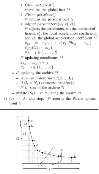
Fig. 1. AMOPSO Diversity computation
B. Update
The Step 2 of AMOPSO deals with the flight of the particles within the swarm through the search space. The flight, given by Equations 1 and 2, is influenced by many vital parameters, which are explained below:
1) Personal Best Performance (pbest): In multi-objective
PSO, the pbest stores the best non-dominated solution
at-tained by the individual particle. In AMOPSO the present
solution is compared with thepbestsolution, and it replaces
thepbestsolution only if it dominates that solution.
2) Global Best Performance (gbest) : In multi-objective PSO, often the multiple objectives involved in MOO prob-lems are conflicting in nature thus making the choice of a single optimal solution difficult. To resolve this problem the concept of non-dominance is used. Therefore instead of having just one individual solution as the global best a set of all the non-dominated solutions is maintained in the
form of an archive [11]. Selecting a single particle from
the archive as the gbest is a vital issue. There has been a
number of attempts to address this issue, some of which may be found in [16]. In the concepts mentioned in [16], authors have considered non-dominance in the selection of thegbestsolution. As the attainment of proper diversity is the second objective of MOO, it has been used in AMOPSO to select the most sparsely populated solution from the archive
as the gbest. In AMOPSO the diversity measurement has
been done using a novel concept. This concept is similar to the crowding-distancemeasure in [14]. The parameter (di) is computed as the distance of each solution to its immediate
next neighbor summed over each of the M objectives.
An example in Figure 1 illustrates the computation of di
parameter. Density for all the solutions in the archive is obtained. Based on the density values as fitness, roulette
wheel selection is done to select a solution as thegbest.
3) Control Parameters (w): The performance of PSO
to a large extent depends on its inertia weight (w) and
the acceleration coefficients (c1 and c2). In this
arti-cle these are called control parameters. These
parame-ters in AMOPSO have been adjusted using the function
adjust parameters(wi, ci
1, ci2).
Some values have been suggested for these parameters in the literature [4]. In most of the cases the values of these parameters were found to be problem specific, signifying the use of adaptive parameters [3], [4], [17]. In this article a novel concept for adapting the control parameters has been proposed. These control parameters have been subjected to optimization through swarming, in parallel with that of the normal optimization variables. The intuition behind this concept is to evolve the control parameters also so that the appropriate values of these parameters may be obtained for a specific problem. Here the control parameters have been initially assigned some random values in the range suggested in [4]. They are then updated using the following equations:
vc
i,j=wivci,j+c1ir1(pci,j−xci,j) +ci2r2(pcg,j−xci,j) (3) xc
i,j =xci,j+vci,j (4)
Here,xc
i,j is the value of thejthcontrol parameter with the
ith particle, whereasvc
i,j,pci,j are the velocity and personal
best for the jth control variable with ith particle. pc
g,j is
the global best for thejth control parameters. The previous
iteration values of the control parameters have been used for
the corresponding values ofwi,ci
1 andci2. It is to be noted
that in the above equations the values of j equal to, 1, 2
and3, corresponds to the control parameters inertia weight,
cognition acceleration coefficient and the global acceleration coefficient respectively. Note that the control parameters for the flight of a particle are taken from its own copy of control variables.
4) Mutation: Themutationoperator plays a key role in MOPSOs [11]. In this article a mutation operator of [13] has been used to allow better exploration of the search space.
5) Update Archive: The selection of the gbest solution for the velocity update is done from this archive only. In AMOPSO the maximum size of the archive has been fixed toNa= 100. The archive gets updated by the non dominated solutions of the swarm. All the dominated members from the archive are removed. Since the maximum size of the archive has been fixed, the density has been considered as in [11] to truncate the archive to the desired size.
After running AMOPSO for a fixed number of iterations, the archive is returned as the resultant non dominated set.
IV. EXPERIMENTALRESULTS
The effectiveness of AMOPSO has been demonstrated on various standard test problems, that have known set of Pareto optimal solutions and are characterized to test the algorithms on different aspects of performance. AMOPSO has been compared with some MOEAs and MOPSOs. The MOEAs include NSGA-II and
PESA-II, whereas the MOPSOs are MOPSO, σ-MOPSO and
NSPSO. The codes for NSGA-II and MOPSO have been
obtained from http://www.iitk.ac.in/kangal/codes.shtml and
http://www.lania.mx/ ccoello/EMOO/EMOOsoftware.html re-spectively. The program for PESA-II has been obtained from the authors, whereas the other algorithms are implemented.
The parameters used are: population/swarm size 100 for
NSGA-II and NSPSO, 10 for PESA-II (as suggested in [15] ),
50 for MOPSO,σ-MOPSO and AMOPSO, archive size 100
for PESA-II,σ-MOPSO, MOPSO and AMOPSO, number of
iterations 250 for NSGA-II and NSPSO, 2500 for PESA-II,
and 500 for MOPSO, σ-MOPSO and AMOPSO (to keep
the number of function evaluations to 25000 for all the algorithms), cross-over probability 0.9 (as suggested in [14]) for NSGA-II and PESA-II, mutation probability inversely proportional to the chromosome length (as suggested in [14]), coding strategy binary for PESA-II (only binary version available) while real encoding is used for NSGA-II, NSPSO,
σ-MOPSO, MOPSO and AMOPSO (PSO naturally operates
on real numbers). The values ofc1andc2have been used as1
and2forσ-MOPSO and NSPSO, respectively (as suggested
in [9] and [10] ). The value ofwhas been used as0.4forσ
-MOPSO whereas it has been allowed to decrease from1.0to
0.4for NSPSO (as suggested in [9] and [10]). For AMOPSO
the initial range of the values forci
1 andci2 is[0.5,2.5]and
that forwiis[0.0,1.0]( as suggested in [17]).
The values for the parameters of a particular algorithm have been used keeping in mind the suggestions in the respective literature. Usually a smaller size of the swarm is preferred. The relative performances of NSGA-II, PESA-II,
σ-MOPSO, NSPSO, MOPSO and AMOPSO are evaluated
on several test problems (i.e., two and three objectives), using some performance measures.
A. Test Problems and Performance Measures
In this article nine standard test problems have been used.
Seven of these test problems SCH1, SCH2, F ON [1],
ZDT1,ZDT2,ZDT3,ZDT4[18] are of two objectives,
of three objectives. The performance of the algorithms is
evaluated with respect to the convergence measure Υ(viz.,
distance metric) and the diversity measureΔ[14] (viz.,
di-versity metric). TheΥmeasure has been used for evaluating
the extent of the convergence to the Pareto front, whereas
Δmeasure has been used for evaluating the diversity of the
solutions on the non-dominated set. It should be noted that smaller the value of these parameters, the better will be the performance.
B. Results
The results are reported in terms of the mean and variance of the performance measures over 20 simulations in Tables I and II. It can be seen that AMOPSO has resulted in better
convergence on all the test problems in terms ofΥmeasure
except for theSCH1test problem where it is found to be
second to the NSGA-II algorithm. PESA-II has also given the
best convergence for theZDT2test problem. Similarly, the
values of theΔmeasure in Table II show that AMOPSO is
able to attain the best distribution of the solutions on the
non-dominated front for all the test problems except onF ONand
DLT Z2, where it is second to the NSGA-II andσ-MOPSO respectively.
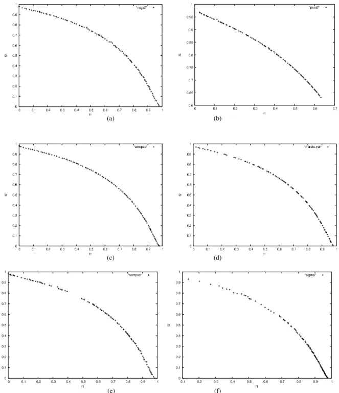
To demonstrate the distribution of the solutions on the final
non-dominated front,F ON,ZDT3andDLT Z2test
prob-lems have been considered as typical illustrations. Figures 2-4 show the resultant non dominated fronts corresponding to these test problems. Figure 2 provides the non-dominated
solutions returned by the six algorithms for theF ON test
problem. The poor performance of PESA-II andσ-MOPSO
is clearly evident. Figure 2(f) shows that σ-MOPSO has
resulted in poor diversity amongst the solutions of the non-dominated set. Although, the results in Figure 2(a), Fig-ure 2(d) and FigFig-ure 2(e) are better than the aforementioned results, the best result has been obtained by AMOPSO in Figure 2(c), in terms of convergence as well as diversity.
Similarly, Figure 3 represents the final fronts obtained
by the six algorithms for ZDT3function. It can be seen
from Figure 3(f) that σ-MOPSO has failed to converge
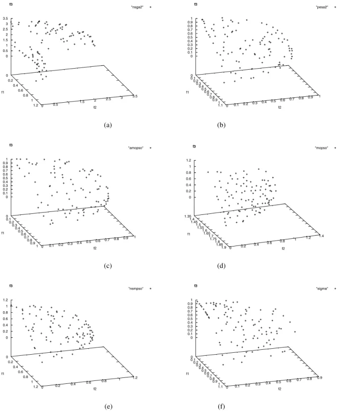
to the true Pareto-front properly. It should be noted from Figure 3(b) that PESA-II has failed to obtain all the five disconnected Pareto-optimal fronts. Although, NSGA-II has been successful in obtaining the five fronts, one of these did not come out properly (Figure 3(a)). MOPSO is found to be better than PESA-II and NSGA-II in this regard, but its solutions have poor spread on the front as is clearly evident from Figure 3(d). Moreover MOPSO is often found to converge to a local optimal front for this test function. Such an instance is shown in Figure 3(g), where MOPSO has been able to obtain only one front (not all the five) because of local optima problem. NSPSO has resulted in very good convergence, as evident from Figure 3(e), but its diversity is not as good as that of AMOPSO. Compared to all these algorithms, AMOPSO in Figure 3(c) has given better convergence and spread of the solutions on this test function. Figure 4 represents the final non-dominated fronts obtained
by the algorithms onDLT Z2test problem. From Figure 4(a)
it can be seen that NSGA-II has failed considerably in attaining the non-dominated set properly in terms of both convergence as well as diversity. MOPSO (Figure 4(d)) has
failed to attain the full non-dominated set. Similarly σ
-MOPSO (Figure 4(f)) could not attain the non-dominated set properly. Although NSPSO has resulted in better shape of the Pareto front (Figure 4(e)), its convergence is not as good as that of AMOPSO and PESA-II as shown in Figure 4(c) and Figure 4(b) respectively.
V. CONCLUSIONS ANDDISCUSSION
In the present article, a novel multi-objective PSO algo-rithm, called AMOPSO, has been presented. AMOPSO is adaptive in nature with respect to its inertia weight and acceleration coefficients. This adaptiveness enables it to attain a good balance between exploration and exploitation of the search space. A mutation operator has been incorporated in AMOPSO to resolve the problem of premature conver-gence to the local Pareto-optimal front (often observed in multi-objective PSOs). An archive has been maintained to store the non-dominated solutions found during AMOPSO
execution. The selection of thegbestsolution is done from
this archive, using the diversity consideration. The method for computing diversity of the solutions is based on the nearest neighbor concept. The performance of AMOPSO is compared with some recently developed multi-objective PSO techniques and evolutionary algorithms, for nine function optimization problems of two and three objectives using some performance measures. AMOPSO is found to be good not only in approximating the Pareto optimal front, but also in terms of diversity of the solutions on the front.
In this article only one version of the adaptation of control parameters has been addressed, where each particle has its own control parameter. This form of adaptation can be
achieved at other levels also, like atpbestandgbestlevel.
Further it would be interesting to study the values of these control parameters finally when the non dominated front is obtained.
REFERENCES
[1] K. Deb,Multi-Objective Optimization usingEvolutionaryAlgorithms. John Wiley and Sons, USA, 2001.
[2] J.Kennedy and R. Eberhart, “Particle Swarm Optimization,” inIEEE International Conference Neural Networks, 1995, pp. 1942–1948. [3] A. P. Engelbrecht, Fundamentals of Computational Swarm
Intelli-gence. John Wiley and Sons, USA, January 2006.
[4] F. van den Bergh, “An analysis of particle swarm optimizers,” Ph.D. dissertation, Faculty of Natural and Agricultural Science, University of Pretoria, Pretoria, November 2001.
[5] X. Hu and R. Eberhart, “Multiobjective Optimization Using Dynamic Neighbourhood Particle Swarm Optimization,” inProceedings of the 2002 Congress on EvolutionaryComputation, part of the 2002 IEEE World Congress on Computational Intelligence. Hawaii: IEEE Press, May 2002, pp. 12–17.
[6] K. Parsopoulos and M. Vrahatis, “Particle swarm optimization method in multiobjective problems,” inProceedings of the 2002 ACM Sy mpo-sium on Applied Computing(SAC 2002), 2002, pp. 603–607. [7] C. Coello and M. Lechuga, “MOPSO: A Proposal for Multiple
Objective Particle Swarm Optimization,” inProceedings of the 2002 Congress on EvolutionaryComputation, part of the 2002 IEEE World Congress on Computational Intelligence. Hawaii: IEEE Press, May 2002, pp. 1051–1056.
TABLE I
MEAN(M)ANDVARIANCE(VAR)OF THEΥMEASURES FOR THE TEST PROBLEMS
ΥMeasure Algorithm SCH1 SCH2 FON ZDT1 ZDT2 ZDT3 ZDT4 DLTZ2 DLTZ7 NSGA-II(M) 0.00339 0.01644 0.00193 0.03348 0.07239 0.11450 0.51305 0.72775 0.04976 (VAR) 0.00000 0.00000 0.00000 0.00475 0.03168 0.00794 0.11846 0.20400 0.00000 PESA-II(M) 0.01687 0.00962 0.02002 0.00105 0.00074 0.00789 9.98254 0.03219 0.05139 (VAR) 0.00000 0.00000 0.00000 0.00000 0.00000 0.00011 20.13400 0.00000 0.00000 σ-MOPSO(M) 0.01364 0.01516 0.00125 0.01638 0.00584 0.10205 3.83344 0.03167 0.24494 (VAR) 0.00000 0.00000 0.00000 0.00048 0.00000 0.00238 1.87129 0.00000 0.01126 NSPSO(M) 0.01002 0.00854 0.00255 0.00642 0.00951 0.00491 4.95775 0.04938 0.05618 (VAR) 0.00000 0.00000 0.00000 0.00000 0.00000 0.00000 7.43601 0.00000 0.00019 MOPSO(M) 0.01148 0.01405 0.00122 0.00133 0.00089 0.00418 7.37429 0.82799 0.04986 (VAR) 0.00000 0.00000 0.00000 0.00000 0.00000 0.00000 5.48286 0.01133 0.00000 AMOPSO(M) 0.00800 0.00554 0.00120 0.00099 0.00074 0.00391 0.40311 0.02024 0.02306 (VAR) 0.00000 0.00000 0.00000 0.00000 0.00000 0.00000 0.01259 0.00000 0.00000 TABLE II
MEAN(M)ANDVARIANCE(VAR)OF THEΔMEASURES FOR THE TEST PROBLEMS
ΔMeasure Algorithm SCH1 SCH2 FON ZDT1 ZDT2 ZDT3 ZDT4 DLTZ2 DLTZ7 NSGA-II(M) 0.47789 1.22823 0.37806 0.39031 0.43077 0.73854 0.70261 0.97599 0.89149 (VAR) 0.00347 0.06216 0.00064 0.00187 0.00472 0.01971 0.06465 0.00738 0.00052 PESA-II(M) 0.65025 1.24480 0.85217 0.84816 0.89292 1.22731 1.01136 0.74808 0.74791 (VAR) 0.01298 0.06092 0.00032 0.00287 0.00574 0.02925 0.00072 0.00093 0.00106 σ-MOPSO(M) 0.60937 1.47054 0.85813 0.39856 0.38927 0.76016 0.82842 0.60405 0.94113 (VAR) 0.02237 0.03025 0.00172 0.00731 0.00458 0.00349 0.00054 0.00194 0.00640 NSPSO(M) 0.39165 1.07167 0.78024 0.90695 0.92156 0.62072 0.96462 0.72988 0.73812 (VAR) 0.00494 0.04239 0.00013 0.00000 0.00012 0.00069 0.00156 0.00091 0.01002 MOPSO(M) 0.76097 1.43353 0.84943 0.68132 0.63922 0.83195 0.96194 0.74808 0.87375 (VAR) 0.016427 0.03504 0.00016 0.01335 0.00114 0.00892 0.00114 0.00093 0.08186 AMOPSO(M) 0.32074 0.96105 0.72422 0.31826 0.31996 0.53154 0.65060 0.67273 0.73201 (VAR) 0.00023 0.00003 0.00003 0.00060 0.00068 0.00036 0.00376 0.00087 0.00134
[8] J. Fieldsend and S.Singh, “A Multi-Objective Algorithm based upon Particle Swarm Optimization, an Efficient Data Structure and Turbu-lence,” inProceedings of UK Workshop on Computational Intelligence (UKCI’02), vol. 2-4, Bermingham, UK, September 2002, pp. 37–44. [9] S. Mostaghim and J. Teich, “Strategies for Finding Good Local Guides
in Multi-objective Particle Swarm Optimization (MOPSO),” inSwarm Intelligence Symposium 2003. SIS’03. Inidanapolis , Indiana, USA: IEEE Service Center, April 2003 2003, pp. 26–33.
[10] X. Li, “A Non-dominated Sorting Particle Swarm Optimizer for Multi-objective Optimization,” in Proceedings of the Genetic and EvolutionaryComputation Conference (GECCO’2003), ser. Lecture Notes in Computer Science, vol. 2723. Springer, 2003, pp. 37–48. [11] C. A. C. Coello, G. T. Pulido, and M. S. Lechuga, “Handling Multiple
Objectives With Particle Swarm Optimization,”IEEE Transactions on EvolutionaryComputation, vol. 8, no. 3, pp. 256–279, June 2004. [12] M. Reyes-Sierra and C. A. C. Coello, “Multi-Objective Particle Swarm
Optimizers: A Survey of The State-of-the-Art,”International Journal of Computational Intelligence Research,, vol. 2, no. 3, pp. 287–308, 2006.
[13] Z. Michalewicz, Genetic Algorithms + Data Structure = Evolution Programs. Springer-Verlag, 1992.
[14] K. Deb, A. Pratap, S. Agarwal, and T. Meyarivan, “A Fast and Elitist Multi-objective Genetic Algorithm: NSGA-II,”IEEE Transactions On EvolutionaryComputation, vol. 6, no. 2, pp. 182–197, April 2002. [15] D. W. Corne, N. R. Jerram, J. D. Knowles, and M. J. Oates, “PESA-II:
Region-based Selection in Evolutionary Multiobjective Optimization,” inProceedings of the Genetic and EvolutionaryComputingConference
(GECCO-2001). Morgan Kaufmann, 2001, pp. 283–290. [16] J. E. Alvarez-Benitez, R. M. Everson, and J. E. Fieldsend, “A MOPSO
Algorithm Based Exclusively on Pareto Dominance Concepts.” in
EMO, 2005, pp. 459–473.
[17] A. Ratnaweera, S. K. Halgamuge, and H. C. Watson, “Self-Organizing Hierarchical Particle Swarm Optimizer with Time-Varying Accelera-tion Coefficients,”IEEE Transactions On EvolutionaryComputation, vol. 8, no. 3, pp. 240–255, June 2004.
[18] E. Zitzler, K. Deb, and L. Thiele, “Comparison of Multiobjective Evo-lutionary Algorithms: Empirical Results,”EvolutionaryComputation Journal, vol. 8, no. 2, pp. 125–148, 2000.
[19] K. Deb, L. Thiele, M. Laumanns, and E. Zitzler, “Scalable Test Problems for Evolutionary Multi-Objective Optimization,” Institut fur Technische Informatik und Kommunikationsnetze,, ETH Zurich Gloriastrasse 35., ETH-Zentrum, CH-8092, Zurich, Switzerland, Tech. Rep. TIK-Technical Report No. 112, July 2001.
(a) (b) (c) (d) 0 0.1 0.2 0.3 0.4 0.5 0.6 0.7 0.8 0.9 1 0 0.1 0.2 0.3 0.4 0.5 0.6 0.7 0.8 0.9 1 f2 f1 "nsmpso" 0 0.1 0.2 0.3 0.4 0.5 0.6 0.7 0.8 0.9 1 0.1 0.2 0.3 0.4 0.5 0.6 0.7 0.8 0.9 1 f2 f1 "sigma" (e) (f)
(a) (b) (c) (d) -0.8 -0.6 -0.4 -0.2 0 0.2 0.4 0.6 0.8 1 0 0.1 0.2 0.3 0.4 0.5 0.6 0.7 0.8 0.9 f2 f1 "nsmpso" -0.5 0 0.5 1 1.5 2 0 0.1 0.2 0.3 0.4 0.5 0.6 0.7 0.8 0.9 f2 f1 "sigma_mopso" (e) (f)
0 0.2 0.4 0.6 0.8 1 1.2 0 0.5 1 1.5 2 2.5 3 3.5 0 0.5 1 1.5 2 2.5 3 3.5 f3 "nsga2" f1 f2 f3 0 0.1 0.2 0.3 0.4 0.5 0.6 0.7 0.8 0.9 1 1.1 0 0.1 0.2 0.3 0.4 0.5 0.6 0.7 0.8 0.9 1 0 0.1 0.2 0.3 0.4 0.5 0.6 0.7 0.8 0.9 1 f3 "pesa2" f1 f2 f3 (a) (b) 0 0.1 0.2 0.3 0.4 0.5 0.6 0.7 0.8 0.9 1 0 0.1 0.2 0.3 0.4 0.5 0.6 0.7 0.8 0.9 1 0 0.1 0.2 0.3 0.4 0.5 0.6 0.7 0.8 0.9 1 f3 "amopso" f1 f2 f3 1.35 1.4 1.45 1.5 1.55 1.6 1.65 1.7 1.75 1.8 1.85 1.9 0 0.2 0.4 0.6 0.8 1 1.2 1.4 0 0.2 0.4 0.6 0.8 1 1.2 f3 "mopso" f1 f2 f3 (c) (d) 0 0.2 0.4 0.6 0.8 1 1.2 0 0.2 0.4 0.6 0.8 1 1.2 0 0.2 0.4 0.6 0.8 1 1.2 f3 "nsmpso" f1 f2 f3 0 0.1 0.2 0.3 0.4 0.5 0.6 0.7 0.8 0.9 1 1.1 0 0.1 0.2 0.3 0.4 0.5 0.6 0.7 0.8 0.9 0 0.1 0.2 0.3 0.4 0.5 0.6 0.7 0.8 0.9 1 f3 "sigma" f1 f2 f3 (e) (f)