An Individualized Preprocessing for Medical Data Classification

(1)

Procedia Computer Science 82 ( 2016 ) 35 – 42

Peer-review under responsibility of the Organizing Committee of SDMA2016 doi: 10.1016/j.procs.2016.04.006

ScienceDirect

Symposium on Data Mining Applications, SDMA2016, 30 March 2016, Riyadh, Saudi Arabia

An individualized preprocessing for medical data classiﬁcation

Sarab AlMuhaideb

a

, Mohamed El Bachir Menai

b a_{Department of Computer Science, Prince Sultan University, 66833 Riyadh 11586, SA}

b_{Department of Computer Science, King Saud University, 51178, Riyadh 11543, SA}

Abstract

Data preprocessing has a profound effect on the performance of the learner. Before attempting medical data classification, charac-teristics of medical datasets, including noise, incompleteness, and the existence of multiple and possibly irrelevant features, need to be addressed. In this paper, we show that selecting the right combination of preprocessing methods has a considerable impact on the classification potential of a dataset. The preprocessing operations considered include the discretization of numeric attributes, the selection of attribute subset(s), and the handling of missing values. The classification is performed by an ant colony optimiza-tion algorithm as a case study. Experimental results on 25 real-world medical datasets show that a significant relative improvement in predictive accuracy, exceeding 60% in some cases, is obtained.

c

2016 The Authors. Published by Elsevier B.V.

Peer-review under responsibility of the Organizing Committee of SDMA2016.

Keywords: classiﬁcation; ant colony optimization; medical data classiﬁcation; preprocessing; feature subset selection; discretization.

1. Introduction

Medical data classification (MDC) refers to learning classification models from medical datasets and aims to improve the quality of health care1_{. Medical data classification can be used for diagnosis and prognosis purposes.}

Medical data exhibit unique features including noise resulting from human as well as systematic errors, missing values and even sparseness2_{. The quality of data has a large implication for the quality of the mining results. It is necessary}

to perform preprocessing steps in order to remove or at least alleviate some of the problems associated with medical data. However, each dataset is different, and there is no preprocessing method that is best across all datasets. Deciding the best combination of preprocessing methods for a specific dataset is not possible without trial and comparisons. The advent of various open-source libraries, like Weka3_{and KEEL}4_{, hosting an extensive set of o}_ff_{-the-shelf preprocessing}

methods, combined with the leisure of standard formats like the attribute-relation ﬁle format (ARFF)1_{and advances in}

computer hardware technology, encourages integration of automatic tuning for preprocessing operations into the data mining task for each dataset on an individual basis. In this research, we investigate the inﬂuence of individualized preprocessing on the classiﬁcation of medical datasets, including the removal of missing values and a variety of

∗_{Corresponding author. Tel.:}₊_{0-966-494-8360 ; fax:}₊_{0-966-454-8317.} E-mail address:[email protected]

1_{http://weka.wikispaces.com/ARFF}

(2)

discretization and attribute selection methods. The rest of the paper is organized as follows. Section 2 highlights related work in the area. Next, Section 3 describes the individualized tuning procedure. Experimental results are presented in Section 4 and discussed in Section 5. The paper is concluded in Section 6.

2. Related Work

Metaheuristic methods stand as interesting techniques for classiﬁcation model learning, because of their good performance and low computational requirements. Metaheuristics require little or no background knowledge of the problem at hand. In ant colony optimization algorithms5,6_{, artiﬁcial ants use pheromone trails and heuristic}

informa-tion to guide soluinforma-tion construcinforma-tion for ﬁnding the shortest path from food sources to their nest. AntMiner7_{is the ﬁrst}

ACO algorithm for classiﬁcation tasks. Among the diﬀerent variants of AntMiner, AntMiner+8_{has been chosen as the}

classiﬁcation algorithm in this research. AntMiner+is based on the MAX–MIN ant system6_{, which is recognized as}

one of the best-performing algorithms in the ant colony optimization family. The classiﬁcation model is constructed using the sequential covering strategy. The results reported show that AntMiner+, on average, obtained the highest rank among state-of-the-art rule-based classiﬁers included8_.

Although the problems associated with medical data have been documented since the nineties, not much research has been done to address the complete preprocessing task of medical data. Tanwani and Farooq2 _{performed an}

extensive study to present the challenges associated with biomedical data and approximate the classification potential of a biomedical dataset using a qualitative measure of this complexity. The study concludes that the classification accuracy is found to be dependent on the complexity of the biomedical dataset, not on the classifier choice. The number and type of attributes have no noticeable effect on the classification accuracy, as compared to the quality of the attributes. It is shown that biomedical datasets are noisy and that noise is the dominant factor that affects the resulting classification accuracy. Lin and Haug9_{use heuristic rules that utilize that utilizes information from the medical data,}

metadata and sources of medical knowledge. As far as we are concerned, the individualized preprocessing of medical data has not been addressed before.

3. An Individualized Preprocessing Procedure

The AntMiner+ is based on a sequential-covering strategy and a default rule related to the majority class. In effect, rule induction focuses on classes other than the majority class. This particular strategy is advantageous in MDC because the majority of class instances are normally the negative cases of which we care less. The sequential-covering strategy helps in handling large-sized datasets; due to the removal of instances already covered by induced rules, the progressive reduction of the training set size is thus achieved. AntMiner+algorithm cannot handle instances containing missing values. Thus, these instances are removed from the dataset in the first step. To reduce the size of the solution space, the number of attributes is limited to no more than a default value of 10. If the dataset contains a larger number of attributes, then attribute selection takes place prior to induction. Various attribute types can be handled by the AntMiner+algorithm. These include nominal and ordinal values, as well as numeric values, including integer and continuous attributes that are discretized. In effect, numeric values are encoded as discrete intervals defined by [lower bound−upper bound]. The order of preprocessing steps in the concerned AntMiner+implementation is as follows: removal of instances with missing values, discretization, then attribute selection.

3.1. Timing of Removing Instances Having Missing Values

In the context of the AntMiner+ algorithm, all instances having missing values are removed in the ﬁrst step of preprocessing. The next steps in the preprocessing consist of the application of the discretization algorithm and attribute selection algorithm (if necessary). This procedure might not be the best in some cases. For example, consider datasets with large number of predictive attributes. If the removal of instances having missing values is delayed after the attribute selection step, then this would allow more instances to be available for training and testing subsets, thus perhaps improving the results. Otherwise, some instances would be removed because they include missing values in attributes that will be next removed by the attribute selection step. Thus, the removal of these instances is no longer rationalized. We hypothesize that if the removal of instances with missing values were delayed until after the attribute selection step, then better results would be obtained.

(3)

3.2. Discretization Method

Diﬀerent discretization methods exist, but none can prove to be the best across all problems and learners10_{. When}

dealing with a specific problem or dataset, the choice of the discretization method has a considerable effect on the classification results in terms of both predictive accuracy and model simplicity.

Four discretization methods were selected for discretization tuning as follows. 1. Fayyad and Irani Discretizer (fay)11_.

2. Kononenko’s MDL Discretizer (kon)12_.

3. EqualWidth Discretizer (eib)13. EqualWidth, or equal interval binning (eib), partitions the continuous domain into a predeﬁned number of equal-width bins. For each dataset, a number of 5, 10, 15, and 20 intervals are examined. The resulting models are referred to as eib5, eib10, eib15, and eib20, respectively.

4. EqualFrequency Discretizer (efb)13_{EqualFrequency, or equal frequency binning (efb), partitions the continuous}

domain into a predeﬁned number of intervals such that the intervals have an equal number of values. Similar to eib, for each dataset, a number of 5, 10, 15, and 20 intervals are examined. The resulting models are referred to as efb5, efb10, efb15, and efb20, respectively.

3.3. Feature Subset Selection Method

Feature subset selection (FSS) finds the minimum subset of features that are useful for the classification process. Further, in medical diagnosis, it is desirable to select the clinical tests that have the least cost and risk and that are significantly important for determining the class of the disease. Following is a list of the considered FSS methods: ReliefF attribute evaluation (rel)14,15_{, correlation-based feature subset selection (cfs)}16_{, consistency subset evaluation}

(con)17, Chi-squared attribute evaluation (chi), gain ration attribute evaluation (gai), information gain attribute eval-uation (inf), OneR attribute evaleval-uation (1R), symmetrical uncertainty attribute evaleval-uation (sym)18_{, and no attribute}

selection employed (AS0).

4. Experimental Results

The implementation of the AntMiner+ algorithm from the AntMiner+ website2 19 is adopted with the same rec-ommended settings. The above-described implementation uses a reasonable set of methods from the open-source Machine Learning Software Weka3_{. We choose to perform the tuning of these steps in the same order of that used for}

their processing in AntMiner+implementation. This allows the tuning for attribute selection to be done when numeric attributes are in the same form that will be used for rule induction. The stratified 10-time, 10-fold cross-validation procedure is used. The Wilcoxon signed-ranks test20 is used for pairwise model analysis. The Friedman test21 is used for multiple comparison tests. Datasets having statistically significant difference among their different models are marked with an asterisk (*). According to these tests, the winner with a significance levelα=0.05 is stressed in bold typeface.

We use 25 medical datasets obtained from the UCI machine learning repository22_{. The benchmark used hosts}

a wide variety of the characteristics listed above. A summary of the main characteristics is presented in Table 1. For each dataset, the number of instances (Inst.), number of attributes (Attr.) including numeric (Num.) and nominal (Nom.) attributes, and number of classes (Class.) are listed. Also included is the percentage of overall missing values (%MV) computed as (missingvalues_Inst._×_Attr. ×100) and the percentage of instances with missing values (%Inst.MV) computed as (inst.withmissingvalues_Inst. ×100). The last two columns in Table 1 report the class noise (Noise) and imbalance ratio (Imb.Ratio) as reported in Ref.2_{. For those datasets that were not reported in Ref.}2_{, a dash (—) is placed.}

Among the 25 datasets in the benchmark, 15 datasets contain missing values. To test the hypothesis, we conduct the following experiment. We modify AntMiner+such that the removal of instances having missing values is delayed after the attribute selection step. The original AntMiner+failed in ﬁve datasets (h h, h swiss, horse, hypo, and sick). The reason for failing is that there were not enough instances left to generate any folds. In all of these datasets, we note that the percentage of instances containing missing values is very high (98.90%−100.00%). The model in which

2_{http://www.antminerplus.com/}

(4)

removal of missing instances is delayed produced output for all five datasets. However, for those with a relatively low number of attributes (h h and h swiss), the results were considerably poor and produced empty rules in several folds. As for the remaining three datasets (horse, hypo, and sick), results were much better. The large number of associated attributes (22−29) has helped in decreasing the percentage of instances with missing values in the remaining attributes post the attribute selection phase. For the rest of the datasets, the difference in performance among the two models is not considered statistically significant.

Table 1. Summary of medical dataset characteristics

Dataset Inst. Attr. Num. Nom. Class. %MV %Inst. Noise Imb.

MV Ratio arr 452 279 206 73 16 0.32 84.96 11.28 1.57 bcw∗a ₆₉₉ ₉ ₉ ₀ ₂ _0.25 _2.29 _2.72 _1.21 cmc 1473 9 2 7 3 0 0 31.98 1.04 derma 366 34 1 33 6 0.06 2.19 0.82 1.05 echo 132 10 8 2 2 7.37 45.26 6.06 1.24 ecoli 336 7 7 0 8 0 0 6.55 1.25 haber 306 3 2 1 2 0 0 16.67 1.57 h c 303 13 6 7 5 0.18 2.31 17.82 1.37 h h 294 13 6 7 5 27.94 99.7 13.61 1.74 h stat 270 13 7 6 2 0 0 15.19 1.03 h swiss 123 13 6 7 5 17.07 100 32.52 1.14 hep 155 19 6 13 2 5.67 48.39 10.97 2.05 horse 368 22 7 15 2 23.8 98.9 11.96 1.15 hypo∗b ₃₇₇₂ ₂₉ ₇ ₂₂ ₄ _5.41 ₁₀₀ _0.54 _9.99 liver 345 6 6 0 2 0 0 9.86 1.05 ljub 286 9 0 9 2 0.35 3.15 — 2.79 lymph 148 18 0 18 4 0 0 10.81 1.46 mammo 961 4 1 3 2 30.77 13.53 14.15 1.01 new thy 215 5 5 0 3 0 0 2.79 1.78 park 195 22 22 0 2 0 0 — 3.39 pima 768 8 8 0 2 0 0 20.18 1.20 p tumor 339 17 0 17 22 3.9 61.06 — 0.90 sick∗b 3772 29 7 22 2 5.41 100 0.71 7.72 wdbc 569 30 30 0 2 0 0 2.11 1.14 wpbc 198 33 33 0 2 0.06 2.02 13.64 1.76 4.1. Discretization Method

The AntMiner+algorithm cannot directly handle numeric attributes. Discretization is an essential step to transform these numeric attributes into a form that the AntMiner+ algorithm can handle ordinal attributes. This results in 10 models as will be shortly described. The best performing model for each dataset will be outlined. The default discretization method in the implementation adopted is fay. For binning discretization methods, the default number of bins is 10. Only datasets having continuous attributes are included in this experiment (21 datasets).

The predictive accuracy with the associated standard deviation obtained by AntMiner+in combination with each of the used discretization methods is shown in Figure 1. The discretization method selected for each dataset is shown in the same figure. In addition, the predictive accuracy, model size as the product of number of rules and number of terms per rule, and computational time per rule set are averaged over all datasets for each discretization method and shown in Figure 2. The grand average of all 10 discretization methods over the 21 datasets is also displayed. From Figure 1, it can be seen that even for the same learner (AntMiner+), the performance across different datasets differs according to the discretization method used. Among the 21 datasets employed in this experiment, the difference in AntMiner+ performance associated with the 10 models for each dataset and resulting from the use of different discretization methods is found to be statistically significant in 12 datasets. In particular, the difference is quite large in three datasets. Namely, the following is noted: In the h h dataset, the relative improvement obtained by kon over fay exceeds 176% (= 80.17−28.96

28.96 ×100%), in the liver disorder dataset, efb10 improves over the default discretization

method fay for more than 41% in predictive accuracy, and the improvement obtained when using eib5 over the default fay is over 54% for the wpbc dataset as well.

In the remaining nine datasets, the diﬀerence among the 10 models for each dataset is not found to be statistically signiﬁcant. This result is not surprising for the derma dataset. This dataset only has one numeric attribute against 32 nominal attributes. However, for two datasets, namely new thy and wdbc, all the predictive attributes are numeric.

(5)

Fig. 1. Results summary predictive accuracy of discretization tuning

Among the 10 models generated, the best rank was obtained by fay, followed by efb10 the highest number of times (5 : 21 and 4 : 21, respectively). If the four eib models were aggregated (eib5, eib10, eib15, and eib20), then eib would score the best rank in (9 : 21) times followed by efb at (7 : 21). The highest number of times a model is selected belongs to fay and efb10 (4 : 21).

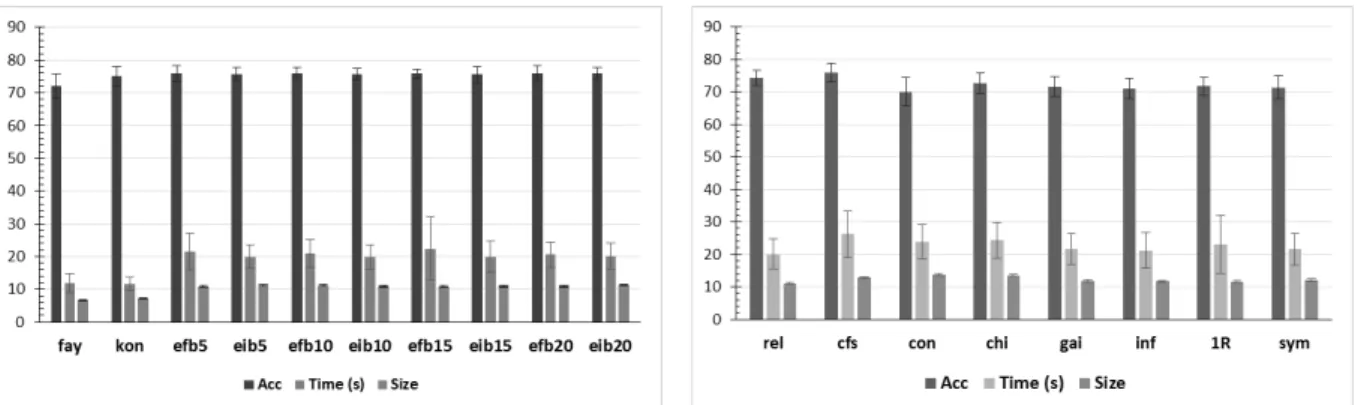
From Figure 2, discretization methods that use binning obtain a higher overall predictive accuracy average over entropy-based methods. These models are also more robust as they have lower overall average standard deviation. The highest average accuracy was obtained by the efb10 method. In addition, the difference among the model sizes obtained is not significant for the 10 models. However, the use of entropy-based discretization methods (fay and kon) results in relatively smaller model sizes. The number of bins does not seem to significantly affect the size of the resulting model. Further, the shortest computational time belong to models using entropy-based discretization methods. Models based on binning discretization methods require almost double the time.

Fig. 2. Average predictive accuracy, model size, and time (s) over all datasets for AntMiner+per discretization method

Fig. 3. Average predictive accuracy, model size, and time (s) over all datasets for AntMiner+per FSS method

4.2. Feature Subset Selection Method

A diverse combination of FSS methods is included in the comparison. Weka java implementation with default settings for attribute selection methods is used. The default feature subset selection method in the implementation19

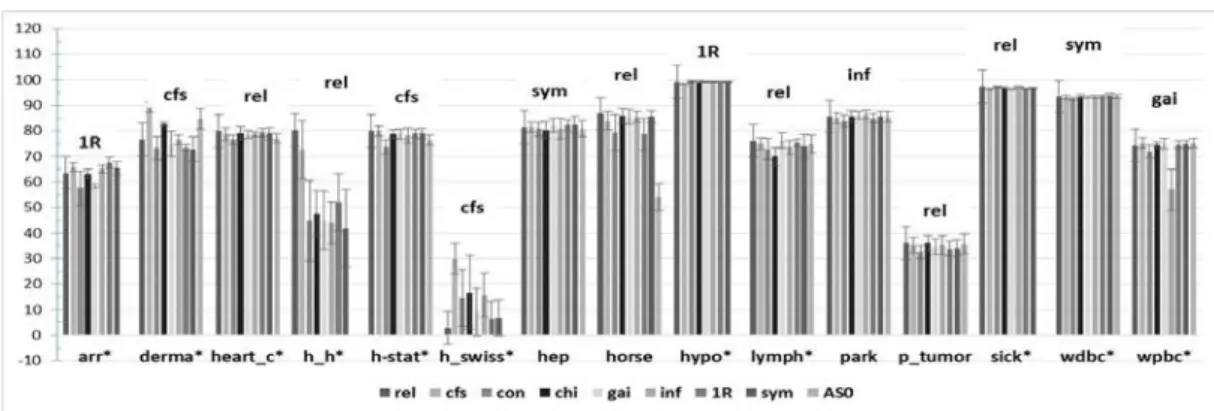
adopted is rel with 10 as the default number of attributes to retain. Therefore, only datasets having more than 10 attributes are included in this experiment (15 datasets). The non-parametric Friedman test is used to test whether the difference among the predictive accuracy of the selected models is considered statistically significant. The statistical comparison is only done among results associated with the eight FSS methods. The model where no attribute se-lection is employed (AS0) is not included in the statistical comparisons. The FSS method associated with the best rank is usually chosen. The predictive accuracy with the associated standard deviation obtained by AntMiner+, in combination with each of the used FSS methods, is shown in Figure 4. The FSS method selected for each dataset is shown in the same figure.

(6)

Fig. 4. FSS tuning experiment results summary

In addition, the predictive accuracy, rule size, and computational time per rule set are averaged over all datasets for each FSS method and shown in Figure 3. The grand average of all the eight FSS methods over the 15 datasets is also reported. Table 2 shows the (AS0) case, where no attribute selection is employed. Averages are limited over the 10 datasets where AntMiner+produced a non-zero output. The corresponding average for all the FSS methods over the same datasets is also shown. Figure 4 shows that three FSS methods equally score the best rank for the hep

Table 2. Averages over all datasets for AntMiner+for FSS vs. all features

Variant Acc Rules T/R Time (s)

All FSS 75.97±2.50 4.39±1.01 3.22±0.29 21.89±5.48

AS0 73.79±2.82 4.99±1.04 3.89±0.50 57.13±9.61

dataset: gai, 1R, and sym. The sym FSS method is chosen as it features the highest average and median among the three FSS methods. From Figure 4 and Table 2, several observations can be drawn. The first observation is noted when comparing rule induction combined with FSS with that of full attributes (AS0). The experiment confirms the benefit of FSS as a preprocessing step in this case. Without FSS, the rule induction process failed entirely in some datasets (h h, h swiss, hypo, and sick). For all these datasets, the percentage of instances having missing values is very large (≥99.7%). Therefore, when the next step of preprocessing (removal of instances with missing values) was performed, no instances were left for induction. Effectively, FSS significantly reduces the percentage of instances having missing values and is thus fundamental in this case. The same reasoning is related to the inferior performance (predictive accuracy) obtained in similar datasets (e.g., horse dataset).

The second conﬁrmed advantage is the acceleration of search when using FSS methods in general. It is noticed that using FSS methods reduces the computational time. For example, this reduction is up to six times in the derma dataset. In general, the computational time of AntMiner+ without FSS is more than twice as much as that obtained by averaging the computational time of AntMiner+combined with each of the eight FSS methods. Also, note that the solution size is larger and the accuracy is on average lower.

When comparing results using the different FSS methods, we note that out of the 15 datasets, the difference among AntMiner+ results, when combined with each of the eight FSS methods, is considered statistically significant in 11 datasets. The high imbalance ratio in some (e.g., hypo and sick) seems not to affect the results. Among these, the difference is extremely significant in h h, h swiss, and wpbc datasets. For example, it can be seen that changing the FSS method used with AntMiner+for the h h dataset can improve the predictive accuracy from (41.82%) when using sym to (80.17%) when using rel, thus effectively providing over 91% improvement in accuracy. These three datasets (h h, h swiss, and wpbc) exhibit the highest level of class noise combined with highest percentage of instances having missing values, and small number of instances (below 300). Most FSS methods showed to be the preferred for at least one dataset, however, the methods rel followed by cfs obtained the largest count of best ranks. When considering grand averages, Figure 3 shows that the highest overall average is associated with the correlation-based FSS method (cfs). It also features the highest computational time. The follow-up is ReliefF method (rel). In all models, comparable rule set sizes are found.

(7)

Fig. 5. Average predictive accuracy for AntMiner+showing the diﬀerence before and after the tuning phase

4.3. Performance of the Tuned AntMiner+

By the end of the tuning phase with its four steps, it is time to compare the results before and after tuning. Figure 5 shows the predictive accuracy along with the standard deviation for the original AntMiner+with the default settings versus those for the tuned version. The ﬁnal model for AntMiner+after tuning is referred to asAM+Tunedhereafter.

5. Discussion

The removal of instances having missing values results in information loss. However, if this step is delayed after FSS, then the percentage of information loss is considerably decreased, thus allowing more instances for the training and testing processes. This conclusion particularly holds for datasets having a larger number of predictor features. The study also found that despite the noise normally associated with medical datasets, providing more instances to the learning algorithm improves the classiﬁcation results.

In this study, it is found that for datasets having more than 10 attributes, using FSS methods always proves fruitful in comparison to induction without FSS. When averaged over all datasets, induction using the cfs FSS method scores the highest predictive accuracy with no payoffin rule set size. When considering different features of the datasets, missing values especially have a strong effect on induction using FSS.

Discretization enhances model comprehensibility and excels the search. It is important to ﬁnd a balance between the number of intervals generated and the performance obtained, as the search space grows exponentially with the number of intervals. Among the discretization methods included in this experiment, the use of entropy-based dis-cretization methods has a computational cost advantage in terms of model complexity and computational time. Dis-cretization methods based on binning obtain overall higher averages in predictive accuracy and lower variance than those based on entropy.

When evaluating the performance ofAM+Tuned, a closer look at Figure 5 shows that no significant difference is encountered in 11 out of the 25 datasets. One interesting result is that there was no improvement obtained at all during the tuning process for the new thy dataset. By investigating the dataset characteristics, we note that it has no missing values, and no attribute selection is needed as it contains only five attributes. The tuning step concluded that the fay discretization method is found to be the best suited. These are the same settings in the Original AntMiner+ implementation, and that explains the situation. In five datasets out of the remaining fourteen datasets (h h, h swiss, horse, hypo, and sick), the difference was of success/failure in obtaining an output. The difference is statistically significant in the nine remaining datasets (arr, cmc, derma, echo, haber, liver, park, p tumor, and wpbc). Thus, in the majority of datasets, there is a significant improvement achieved via the tuning process. The grand average over the 20 datasets in the benchmark, where the output is obtained by AntMiner+Original, shows an overall significant improvement obtained through the tuning process, as confirmed by the Wilcoxon test that was applied to compare the two models (AntMiner+Original [72.65±2.89] andAM+Tuned[78.08±1.74]) for the same 20 datasets.

Although this study speciﬁcally addresses medical datasets, the recommended preprocessing procedure can be applied to arbitrary datasets with similar features. First, the existence of missing values is addressed. If the dataset contains missing values, then the timing of removing instances with missing values should be examined, whether it is done before or after the FSS step. Next, the discretization process is examined. A number of discretization

(8)

methods should be investigated, and the associated classiﬁcation results for the resulting models compared. Once the best model is chosen according to measures of concern such as predictive accuracy or model complexity, FSS step is considered. This step is particularly recommended for datasets with small number of instances but large number of features. Similar to the discretization step, a number of feature subset selection methods is to be explored.

6. Conclusions

This work shows the results of the tuning for the preprocessing stage, which was applied to AntMiner+ as an illustrative example. For each dataset, the timing of removing instances with missing values was examined. Experi-mentations were done with different feature subset selection and discretization methods for each dataset. Experiments show that there is a significant improvement in classification performance measured by predictive accuracy and ob-tained in the majority of datasets in the benchmark through the individualized tuning of the preprocessing operations. Moreover, given a certain classification algorithm, the design of the preprocessing stage can make the difference be-tween complete failure and the achievement of results that are competitive to rival classification algorithms in the same datasets. The real bounty of this step is that improving the classification potential of a dataset is now a convenient problem-centeredapproach to computation.

References

1. AlMuhaideb, S., Menai, M.E.B.. A new hybrid metaheuristic for medical data classiﬁcation.International Journal of Metaheuristics2014; 3(1):59–80.

2. Tanwani, A.K., Farooq, M.. Performance evaluation of evolutionary algorithms in classiﬁcation of biomedical datasets. In: Rothlauf, F., editor.The 11th Annual Conference Companion on Genetic and Evolutionary Computation: Late Breaking Papers, GECCO’09. Canada: ACM; 2009, p. 2617–2624.

3. Milne, D.N., Witten, I.H.. An open-source toolkit for mining wikipedia.Artiﬁcial Intelligence2013;194:222–239.

4. Alcal´a-fdez, J., S´anchez, L., Garc´ıa, S., Jesus, M.J.D., Ventura, S., Garrell, J.M., et al. KEEL: A software tool to assess evolutionary algorithms to data mining problems.Soft Computing2009;13(3):307–318.

5. Dorigo, M., Gambardella, L.M.. Ant Colony System: A Cooperative Learning Approach to the Traveling Salesman Problem. IEEE Transactions on Evolutionary Computation1997;1(1):53–66.

6. St¨utzle, T., Hoos, H.H.. MAX-MIN ant system.Future Generation Computer Systems2000;16(8):889–914.

7. Parpinelli, R.S., Lopes, H.S., Freitas, A.A.. Data mining with an ant colony optimization algorithm. IEEE Transactions Evolutionary Computation2002;6(4):321–332.

8. Martens, D., Backer, M.D., Haesen, R., Vanthienen, J., Snoeck, M., Baesens, B.. Classiﬁcation with ant colony optimization. IEEE Transactions on Evolutionary Computation2007;11(5):651–665.

9. Lin, J.H., Haug, P.J.. Data preparation framework for preprocessing clinical data in data mining. In:AMIA Annu Symp Proc. AMIA; 2006, p. 489–493.

10. Garc´ıa, S., án Luengo, J., Sáez, J.A., López, V., Herrera, F.. A survey of discretization techniques: Taxonomy and empirical analysis in supervised learning.IEEE Transactions on Knowledge and Data Engineering2013;25(4):734–750.

11. Fayyad, U.M., Irani, K.B.. Multi-interval discretization of continuous-valued attributes for classiﬁcation learning. In: International Conference on Artiﬁcial Intelligence. 1993, p. 1022–1029.

12. Kononenko, I.. On biases in estimating multi-valued attributes. In:International Conference on Artiﬁcial Intelligence. Morgan Kaufmann; 1995, p. 1034–1040.

13. Wong, A.K.C., Chiu, D.K.Y.. Synthesizing statistical knowledge from incomplete mixed-mode data. IEEE Transactions Pattern Analysis and Machine Intelligence1987;9(6):796–805. URL:http://dblp.uni-trier.de/db/journals/pami/pami9.html#WongC87. 14. Kira, K., Rendell, L.A.. A practical approach to feature selection. In: Sleeman, D.H., Edwards, P., editors.ML. Morgan Kaufmann. ISBN

1-55860-247-X; 1992, p. 249–256.

15. Kononenko, I.. Estimating attributes: Analysis and extensions of RELIEF. In:European Conference on Machine Learning. Springer Verlag; 1994, p. 171–182.

16. Hall, M.A..Correlation-based Feature Selection for Machine Learning. Ph.D. thesis; University of Waikato; Hamilton, NewZealand; 1999. 17. Liu, H., Setiono, R.. A probabilistic approach to feature selection - a ﬁlter solution. In: Saitta, L., editor.International Conference on

Machine Learning. Morgan Kaufmann. ISBN 1-55860-419-7; 1996, p. 319–327.

18. Frank, E., Witten, I.. Generating accurate rule sets without global optimization. In:Proceedings of the 15th_{International Conference on} Machine Learning. Morgan Kaufmann; 1998, p. 144–151.

19. Minnaert, B., Martens, D., De Baker, M., Baesens, B.. To tune or not to tune: Rule evaluation for metaheuristic-based sequential covering algorithms. Working Paper 12769; Universiteit Gent; 2012.

20. Wilcoxon, F.. Individual comparisons by ranking methods.Biometrics Bulletin1945;1(6):80–83.

21. Friedman, M.. The use of ranks to avoid the assumption of normality implicit in the analysis of variance.American Statistical Association 1937;32(200):675–701.