The optimal regularization and its application in extreme learning machine for regression analysis and multi-class classification

University of Stuttgart

Institute of Geodesy

The Optimal Regularization and its Application

in Extreme Learning Machine for Regression

Analysis and Multi-class Classification

Master Thesis

Geodesy and Geoinformation

University of Stuttgart

Kun Qian

Stuttgart, October 2018

Supervisor: Dr. -Ing. Jianqing Cai University of Stuttgart Prof. Dr.-Ing. Nico Sneeuw University of Stuttgart

Erklärung der Urheberschaft

Ich erkläre hiermit an Eides statt, dass ich die vorliegende Arbeit ohne Hilfe Dritter und ohne Benutzung anderer als der angegebenen Hilfsmittel angefertigt habe; die aus fremden Quellen direkt oder indirekt übernommenen Gedanken sind als solche kenntlich gemacht. Die Arbeit wurde bisher in gleicher oder ähnlicher Form in keiner anderen Prüfungsbehörde vorgelegt und auch noch nicht veröffentlicht.

Ort, Datum Unterschrift

Abstract

Extreme Learning Machine (ELM) proposed by Huang et al. (2006) is a newly de-veloped single layer feed-forward neural network (SLFN). It is attractive for its high training efficiency and satisfactory performance, especially when dealing with a large amount of data, which are often in high-dimensional space. However, current ELM cannot solve the over-fitting problem among other several problems. While minimiz-ing residuals of output errors for the trainminimiz-ing data, it tends to generate an over-fittminimiz-ing model, whose generalization ability is relatively weak. Even if the model fits the train-ing data perfectly, it performs unsatisfactory for the testtrain-ing data. In traintrain-ing process, we aim to minimize residuals of output errors of training data. It tends to generate an over-fitting model, which has poor generalization ability. The model maybe fit the training data perfectly, but performs bad in testing data. Furthermore, in order to im-prove accuracy, the traditional way is increasing the number of hidden-layer neurons, but excessive hidden-layer neurons result in an ill-posed normal matrix and a model which is over sensitive to the change of the training data. In such case, the performance of ELM is significantly affected by the outliers in the training data. In order to over-come these problems, we apply the regularization to the original ELM. In this study, the A-optimal design regularization is performed to improve the generalization ability and stability of ELM. The performance of ELM with the A-optimal design regulariza-tion will be evaluated through two main applicaregulariza-tions, respectively, regression analysis and satellite image multi-class classification.

IX

Contents

List of Figures XI

List of Tables XIII

1 Introduction 1

1.1 Motivation . . . 1

1.2 Outline . . . 2

2 Artificial Neural Networks 3 2.1 Human Brain . . . 3

2.2 Artificial Neurons . . . 4

2.3 Activation Function . . . 7

2.4 Neural Networks Architecture . . . 9

2.5 Learning Process . . . 12

2.6 The Back-Propagation Algorithm . . . 12

3 Extreme Learning Machine and its Regularization 17 3.1 Single Hidden Layer Feed-forward Neural Networks (SLFNs) with Ran-dom Hidden Neurons . . . 18

3.2 Learning with Extreme Learning Machine . . . 19

3.3 Regularization on Extreme Learning Machine . . . 23

4 A-optimal Design Regularization and its Application in ELM 27 4.1 λ−weighted Best Linear Estimation . . . 27

4.2 A-optimal design Regularization . . . 30

5 Case Studies: Application of A-optimal Design Regularization in Extreme Learning Machine 33 5.1 Approximation of Sine Function . . . 33

5.2 Regression Analysis in Real-world Problems . . . 36

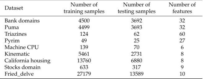
5.3 Multi-class Classification in Satellite Images . . . 39

5.4 Conclusions and Future Works . . . 52

Bibliography XV

XI

List of Figures

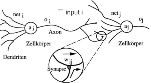
2.1 Essential components of a neuron shown in stylized form; source: Zell

et al. (1993) . . . 4

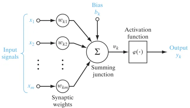
2.2 Nonlinear model of a neuron; source: Haykin (2009) . . . 5

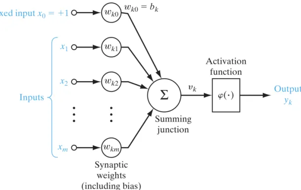
2.3 Nonlinear model of neuron k after refoumulation, ωk0 accounts for the biasbk; source: Haykin (2009) . . . 6

2.4 Threshold Function . . . 7

2.5 Linear activation function . . . 8

2.6 Sigmoid function . . . 9

2.7 Sigmoid function of different slope parameter . . . 9

2.8 2-layer feed-forward neural networks; source: Haykin (2009) . . . 10

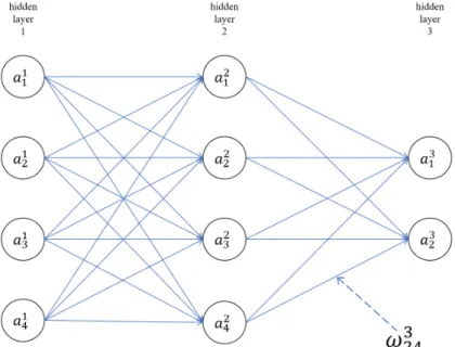
2.9 Single hidden layer feed-forward network (SLFN); source: Haykin (2009) 11 2.10 An example for a weight in multi-layer neural networks: the weight from the 4th _{neuron in the 2}nd _{hidden layer to the 2}nd _{neuron in the 3}rd hidden layer . . . 13

3.1 Relationship between regularizationλand RMSE in validation set . . . 26

4.1 Balance of the variance and the bias by the weighting factor λ; source: Cai (2004) . . . 29

5.1 Approximation of the sine function with both algorithms without outliers 35 5.2 Approximation of the sine function with both algorithms with outliers . 35 5.3 Position of the study area in Wuhan; source: Google Earth . . . 40

5.4 Satellite image of the study area in Wuhan; source: Google Earth . . . . 41

5.5 Satellite image to be classified for study area in Wuhan . . . 44

5.6 Classified study area in Wuhan by the original ELM . . . 45

5.7 Classified study area in Wuhan by the ELM with A-optimal design reg-ularization . . . 46

5.8 Satellite image of study area in Karlsruhe from Google Earth . . . 47

5.9 Satellite image to be classified for study area in Karlsruhe . . . 50

5.10 Classified study area in karlsruhe by the original ELM . . . 51

XIII

List of Tables

5.1 Data Information for Approximation of the Sine Function . . . 34

5.2 Comparison of RMSE of the original ELM and the ELM with A-optimal design regularization in both situations . . . 34

5.3 Specification of the datasets used for regression analysis . . . 36

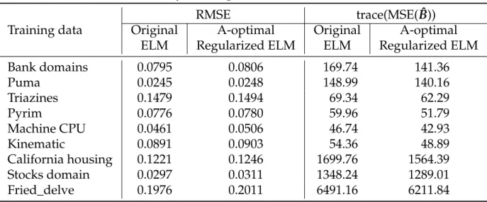
5.4 Results for training data: RMSE and trace(MSE(Bˆ)) . . . 38

5.5 Results for testing data: RMSE . . . 38

5.6 Specification of data information of the study area in Wuhan . . . 42

5.7 Specification of labeled pixels of the study are in Wuhan . . . 42

5.8 Confusion matrix of the classification in the study are in Wuhan by using the original ELM . . . 42

5.9 Confusion matrix of the classification in the study area in Wuhan by using the regularized ELM . . . 43

5.10 Accuracy and Cohens Kappa coefficient of the classification in the study area in Wuhan . . . 44

5.11 Specification of data information of the study area in Karlstuhe . . . 48

5.12 Specification of labeled pixels of the study area in Karlsruhe . . . 48

5.13 Confusion matrix of the classification in the study are in Karlsruhe by using the original ELM . . . 49

5.14 Confusion matrix of the classification in the study are in Karlsruhe by using the regularized ELM . . . 49

5.15 Accuracy and Cohens Kappa coefficient of the classification in the study area in Karlsruhe . . . 50

1

Chapter 1

Introduction

1.1 Motivation

Machine learning has been one of the rapidest developing field of computer science with far-reaching applications since the recent couple of decades. It becomes more and more popular for people to apply machine learning to solve real-life problems efficiently.

Artificial neural network (ANN) plays an important role in machine learning. An ANN is a model of computation, inspired by the structure of neural networks in brain. It provides a general, practical method for learning real-valued, discrete-valued and vector-valued functions from training data (Mitchell, 1997). Learning with ANNs was proposed in the mid-20th century. It formed an efficient learning algorithm and has achieved outstanding performance on many learning tasks (Hierons, 2015).

However, when we deal with a large amount of data in high-dimensional feature space, the training speed of the ANN are seriously affected, if we apply traditional feedforward propagation and back propagation to estimate weight matrices by the stochastic gradient descent. It often takes several or even more days to train the ANN. Besides, gradient descent learning algorithms can easily converge to local minimum, resulting in low accuracy of prediction.

Huang et al. (2006) have proposed extreme learning machine (ELM) to solve such prob-lems mentioned above. It is a special single-hidden layer feedforward neural network (SLFN). Instead of estimating both input and output weight matrices with hundreds of learning iteration, we estimate only the output weight matrix or the output vector in ELM with a randomly initialized input weight matrix. The output weight matrix or the output vector can be estimated by Moore-Penrose generalized inverse with the least squares method.

Granted, ELM has successfully solved lots of real-life problems, which were difficulties for traditional ANNs, but its generalization ability remains unsolved problems, which are common in methods based on feedforward neural networks. In other words, how to acquire appropriate network architecture is the problem that we need to solve. On the one hand, we cannot model the data with sufficiently high accuracy through only a

few layer neurons. On the other hand, a neural network with excessive hidden-layer neurons tends to generate an over-fitting model.

The most common way to improve the generalization performance in machine learn-ing is the regularization. By applylearn-ing the regularization to ELM, it is necessary not only to minimize the sum of the output residuals of the training data, but to penalize the coefficients of the output matrix or the output vector as well. Our challenge is to find a precisely adaptive regularization parameter to balance one with the other. In this study, we apply the A-optimal design regularization to ELM to determine an op-timal regularization parameter, which can address the under-fitting/over-fitting trade-off.

1.2 Outline

The rest of this thesis is organized as follows. Firstly, some basic theories of feed-forward neural networks will be reviewed. For example, feedfeed-forward propagation, back-propagation and stochastic gradient descent. Here we will also talk about the problems of traditional training methods.

In addition, ELM proposed by Huang et al. (2006) will be introduced as a special schema of SLFN. The advantages of ELM over traditional SLFN and how to deal with problems with ELM will be discussed in detail. Moreover, we will emphasize the rea-son why regularization is necessary for ELM here.

In the next chapter, we will talk about how to determine an optimal regularization pa-rameter for ELM by using A-optimal design regularization. The principle of A-optimal design regularization is to be interpreted. Besides, an existing regularization method used in ELM will be reviewed and some main weakness should be discussed.

Finally, we will inspect the performance of ELM with A-optimal design regularization on several case studies and demonstrate the comparison to original ELM.

3

Chapter 2

Artificial Neural Networks

Artificial neural networks are commonly referred to as "neural networks". Work on neural networks has been inspired right from its inception by the consciousness that human brain deal with problems in an entirely different way from digital computers. Human brain is a highly complex, nonlinear, and parallel information-processing sys-tem (Haykin, 2009). In human brain, neurons are known as structural constituents and they are organized to perform certain computation, for example, pattern recognition. And the computation speed of human brain is much faster than the fastest digital com-puter nowadays. To be specific, human brain can deal with complicated recognition tasks in only 100-200 ms, whereas tasks of much less complexity cost a great deal of time on a powerful computer.

A neural network is a machine system that is designed to imitate the way in which human brain performs a particular task or function of interest. The neural network consists of artificial neurons, which have similar function as information-processing units in human brain. In addition, the neural network is implemented in software on digital computers. In order to make neural networks performing useful computations, a massive interconnection of simple artificial neuron should be employed. With such neurons, neural network can acquire and store experimental knowledge, then make it available for handling similar problems. This process is so called learning. The procedure applied to carry out the learning process is named learning algorithm. In this chapter, a basic type of neural networks, called single layer feed-forward neural networks (SLFN) and a traditional learning algorithm for SLFN will be reviewed.

2.1 Human Brain

At the beginning, we take a quick look at some basic neurobiology. A human brain consists of about 100 billion neurons. A highly stylized example of the neuron is shown in figure 2.1. Neurons communicate with each other via electrical signals which are transient impulses. Each neuron typically receives thousands of signals from other neurons. which eventually reach the cell body. Then, the signals are integrated in some

way to generate a voltage impulse for output. The generated impulse is transmitted to other neurons via a branching fibre known as axon.

Figure 2.1:Essential components of a neuron shown in stylized form; source: Zell et al. (1993)

To perform a certain task, for example, pattern recognition, human brain can operate information in highly parallel processes on representation that are distributed over a large amount of neurons. This kind of highly parallel computation or operation based on distributed representation is an important motivation for ANN. With neurobiolog-ical analogy as the source of inspiration, and the wealth of theoretneurobiolog-ical and computa-tional tools that we are developing, it is now possible to simplify networks in human brain as ANN to offer an alternative form of parallel computation that might be more appropriate for solving tasks in real world.

2.2 Artificial Neurons

An artificial neuron, called neuron in brief, in an ANN is an information-processing unit, which is fundamental to the operation of an ANN. Figure 2.2 shows the model of a neuron, which represents the basis for designing a general neural network.

2.2 Artificial Neurons 5

Figure 2.2:Nonlinear model of a neuron; source: Haykin (2009)

From figure 2.2, four basic elements of the model of neurons can be identified:

• A set of connecting links, which are characterized by a weight matrix.

• An adder for summing all input signals, the operation described here constitute

a linear combiner.

• An activation function for limiting the amplitude of the output of an neuron.

Typically, the amplitude range of the output after limitation is within the inter-val [0,1]or alternatively [−1,1], which are depended on the choice of activation

function.

• Bias, which has the effect of increasing or lowering the net input of the activation

function.

We can describe the neuronkdepicted in figure 2.2 mathematically with a pair of equa-tions: uk= m

∑

- ωk is the respective input weight matrix of neuronk.

- uk(not shown in figure 2.2) is the linear combiner output due to the inputs. - ϕis the activation function

- ykis the output of the neuronk

- bkis the bias, which can result in an affine transformation touk If we assume the result ofuk after affine transformation asvk:

vk=uk+bk (2.3)

We can rewrite the equation (2.3) in matrix form as follows. vk =uk+bk = m

∑

Therefore, it is possible to reformulate the model of neuronkas shown in figure 2.3

Figure 2.3: Nonlinear model of neuron k after refoumulation, ω_k0 accounts for the bias b_k; source:

Haykin (2009)

In figure 2.3, the bias is accounted as an input unit, by these 2 operations:

• adding another input unit with constant value +1 • adding a new input weight equal to the biasbk

2.3 Activation Function 7 For such model after reformulation, we can describe it in mathematical terms as equa-tion

yk=ϕ(wk·X) =ϕ(vk) (2.5) - Xis the input adding a constant term with value +1

- wk is the new input weight including the biasbk. - ϕis the activation function.

2.3 Activation Function

Activation functions are an extremely important part of the artificial neural networks. An activation function is also known as transfer function. It maps the resulting values of a neuron in between (0,1) or(−1,1) (depending upon the type of activation

func-tion). The activation functions take the decision whether a neuron should be activated or not, so in other words, the activation functions decide if the input information re-ceived should be passed or ignored. In addition, the activation functions help to trans-form the input intrans-formation non-linearly and it is this non-linearity makes it possible to learn arbitrarily complicated transformation from the input to the output. Therefore, the neural networks are capable to learn and perform complex tasks.

In what follows, some types of activation functions are reviewed.

• Threshold Function (Binary Step Function)

For this type of activation function, described in figure 2.4, it is defined as

ϕ(vk) = 0 x<0 1 x≥0 (2.6) -5 -4 -3 -2 -1 0 1 2 3 4 5 -0.2 0 0.2 0.4 0.6 0.8 1 1.2

If the value ofvkis above zero, then the neuron is activated. Otherwise, the neu-ron is ignored. This function is more theoretical than practical since in most cases the data should be classified into multiple classes rather than binary classified. Moreover, the gradient of the threshold function is equal to zero. This makes the threshold function not so meaningful because we need to use the gradient of the activation function to modify the weight matrices during back-propagation.

• Linear Function

A simplest example for the linear function isy=x, as shown in figure 2.5.

-5 -4 -3 -2 -1 0 1 2 3 4 5 x -5 -4 -3 -2 -1 0 1 2 3 4 5 linear(x)

Figure 2.5:Linear activation function

When we use linear function as the activation function, the activation is propor-tional to the input information. The linear function gives a range of activation rather than binary activation.

There are two main problems for the linear function. In one hand, the gradient of the linear function is constant and not depending on the input information. Similar to the threshold function, it leads to problems in back-propagation. On the other hand, if we have many hidden layer, and each hidden layer is linear activated. Then, no matter how many layers we have, the output of the last layer is just a linear function of the input of the first layer. This means we just lost the ability of stacking layers if we use the linear function as the activation function.

• Nonlinear Functions

These functions are used to separate the data, which is not linearly separable. Nonlinear functions are the most used activation functions. A nonlinear activa-tion funcactiva-tion makes it easy for the model to generalize and adapt with variety of data. There are many different types of nonlinear activation function, for ex-ample, sigmoid function, tanhfunction, Rectified linear unit (Relu), etc. In this thesis, sigmoid function is used as the activation function, so we will discuss sigmoid function in details here.

2.4 Neural Networks Architecture 9 The sigmoid function has the mathematical form ϕ(vk) = _1+e1−a·_vk, whereais the

slope parameter of the sigmoid function. The curve of the sigmoid function is "S-shaped" as shown is figure 2.6. By varying the parametera, sigmoid functions of different slopes can be obtained, as illustrated in figure 2.7. The sigmoid function is the most common form of activation function used in the construction of neural networks. -10 -8 -6 -4 -2 0 2 4 6 8 10 x 0 0.2 0.4 0.6 0.8 1 sigmoid(x)

Figure 2.6:Sigmoid function

-10 -8 -6 -4 -2 0 2 4 6 8 10 x 0 0.2 0.4 0.6 0.8 1 sigmoid(x) a=0.5 a=0.8 a=1 a=2 a=5

Figure 2.7: Sigmoid function of different slope pa-rameter

As alluded above, the sigmoid function takes a real-valued number and squashes" into range(0,1). Moreover, from the figure 2.6 and 2.7, we can see that

large negative numbers become 0 and large positive numbers become 1.

2.4 Neural Networks Architecture

After the introduction of a single neuron in neural networks, we will talk about the architecture of a integrated neural network. In neural networks, we connect a plenty of neurons by hierarchical networks, with the outputs of some neurons being the inputs to others. These networks can be represented as connected layers of nodes. Each nodes in a layer means a neuron. In a fully fledged neural network, there are many such interconnection nodes. These nodes can come in a myriad of different forms. Here, we may introduce two fundamentally different classes of neural network architectures:

(i) 2-Layer Feedforward Neural Networks

2-layer feed-forward neural networks are the simplest form of layered neural networks, and it was first devised by Rosenblatt (1988). For a 2-layer neural network, we have an input layer of source nodes that projects directly onto an output layer of neurons (computation nodes). 2-layer neural network is strictly of a feed-forward type, as illustrated in figure 2.8

Figure 2.8:2-layer feed-forward neural networks; source: Haykin (2009)

Such a neural network has only a single layer of computation neurons. For the input source nodes, there is no computation performed. With 2-layer neural net-works, we can only solve linearly separable problems. For example, it it only capable of classifying patterns into binary class.

This limitation of the 2-layer neural networks leads to the introduction of hidden layers of neural networks, which are a significant feature of multi-layer feed-forward neural networks.

(ii) Multi-Layer Feed-forward Neural Networks

Multi-layer feed-forward neural networks are the second class of neural net-work architectures. They help to overcome many limitation of 2-layer neural networks and have proved useful in a wide variety of applications. Multi-layer feed-forward neural networks were generally not used before mid 1980s by lack of available training algorithm. After back-propagation was proposed by Rumelhart et al. (1988), multi-layer feed-forward neural networks, sometimes call multi-layer perceptron (MLP) networks, have become a mainstay of neural networks research.

The multi-layer feed-forward neural network distinguishes itself by the presence of on or more hidden layer, whose computation nodes are correspondingly called hidden neurons. The term "hidden" refers to the fact that this part is not seen di-rectly from either the input or output of neural networks. The function of hidden neurons is to intervene between the external input and the network output in some particularly useful manner.

Figure 2.9 illustrate a simple architecture of multi-layer feed-forward neural net-works with single hidden layer, which is also called single hidden layer feed-forward networks (SLFN).

2.4 Neural Networks Architecture 11

Figure 2.9:Single hidden layer feed-forward network (SLFN); source: Haykin (2009)

The source nodes in the input layer constitute the input information applied to the neurons in the hidden layer. Typically, the neurons in each hidden layer of multi-layer neural networks receive the outputs from the layer before as the input information and generate the output and transmit to the adjacent forward layer. The set of outputs of the neurons in the output layer of the multi-layer neural network constitute the overall response of the network to the input information supplied by the source nodes in the input layer.

The neural network in figure 2.9 is also said to be fully connected in the sense that every node in each layer of the network is connected to every other node in the adjacent forward layer. In general, three points highlight the basic features of multi-layer feed-forward neural networks as follows.

– For each neuron in multi-layer feed-forward neural networks, there is a non-linear and differentiable activation function.

– Each multi-layer feed-forward neural network contains one or more hidden layers.

– Each multi-layer feed-forward neural network exhibits a high degree of con-nectivity, the extent of which is determined by weight matrices of the net-works.

These features, however, were also responsible for the deficiencies in applications of multi-layer feed-forward neural networks by lack of corresponding leaning algorithm. On the one hand, the presence of a distributed form of nonlinearity and the high connectivity of the networks make the theoretical analysis difficult to undertake. On the other hand, the use of hidden neurons makes the learning process even more difficult to visualize. Briefly, in the learning process, it should

be decided which features of the input information should be represented by the hidden neurons. Therefore, the learning process is made harder since a choice must be made from a larger space of possible functions to represent the input information.

2.5 Learning Process

Before mid 1980s, there was not a generally good idea to solve such problems men-tioned above and apply multi-layer neural networks to deal with complex tasks. In order to train multi-layer neural networks, Rosenblatt (1988) developed a learning al-gorithm called back-propagation, which is now the most popular and widely used learning algorithm. The training proceeds with back-propagation are divided into two phases:

• Forward Phase

In the forward phase, which is also called feed-forward propagation, all weight matrices in the network are pixed and the input information is propagated through the network, and outputs corresponding to the input information is generated in the end. Therefore, in forward phase, changes are only confined to the activation functions. Due to variant activation functions, we will obtain different outputs through the network.

• Backward Phase

The backward phase is the core of the back-propagation. In the backward phase, an output error is produced by comparing the outputs of the network with a sup-posed result. The output error is propagated through the network, again layer by layer, but in backward direction this time. In the backward phase, successive ad-justments are made to the weight matrices of the network.

2.6 The Back-Propagation Algorithm

As it is already mentioned many times previously, the development of the back-propagation provides a computationally efficient method for training multi-layer neural networks. At the heart of back-propagation is an expression for the partial derivative ∂C

∂ω of the cost function C with respect to an weight ω (or bias b) in the

networks. This expression tells us how quickly the cost function Cchanges when the weights and biases are changed. The back-propagation algorithm gives us detailed insights into how changing the weights and biases changes the overall performance of the network.

2.6 The Back-Propagation Algorithm 13

Matrix-based Computation

The matrix-based approach to computing the outputs from a neural network is men-tioned briefly in the previous section. Here, we will revisit the matrix-based com-putation in details. It provides a good way to understand the notation used in the back-propagation algorithm.

We will begin with a notation which refers to weight in the networks. wl_jk is used to denote the weight for the connection from kth neuron in the (l−1)th hidden layer to

the jth neuron in thelthhidden layer. The diagram below shows us an example of the weight on a connection from the 4th _{neuron in the 2}nd _{hidden layer to the 2}nd _neuron in the 3rd_{hidden layer of a network:}

Figure 2.10:An example for a weight in multi-layer neural networks: the weight from the4thneuron in

the2nd_{hidden layer to the2}nd_{neuron in the3}rd_{hidden layer}

Similarly, we usebl_j for the bias and al_j for the activated output of jth neuron in thelth hidden layer. With such notations, the relationship of the activational_jto the activations in the(l−1)thlayer can be presented by the equation (2.7)

al_j=ϕ(

∑

k

wl_jkal_k−1+bl_j) (2.7)

where the sum is over all neurons in the(l−1)thlayer. To rewrite this expression in a

matrix form, we define a weight matrixwl and a bias vector bl for each hidden layer l. It consists of all the weights connecting to the lth layer of neurons. Specifically, the

entry in the jthrow andkth column iswl_jk. Afterwards, we can write the equation (2.7) in compact vectorized form

al=ϕ(wlal−1+bl) (2.8)

Cost Function

The goal of back-propagation is to compute the partial derivatives ∂C

∂w and ∂C

∂b. The

cost function is used to quantify how accurate the computed outputs of the neural networks are, comparing to the corresponding supposed outputs. It has the form

C(w,b) = 1 2n|| n

∑

• n is the number of training samples

• yis the vector of corresponding supposed outputs

• aoutis the computed outputs

Procedure of Back-propagation

In order to compute the partial derivatives ∂C

∂w and ∂C

∂b, it is necessary to introduce an

intermediate,δl_j, which refers to the error in the jthneuron in thelthlayer. δl_j= ∂C

∂zl_j (2.10)

where zl_jis the unactivated output. Then, we useδl to denote the vector of error

asso-ciated with layer l. The back-propagation algorithm gives us a way to computeδl for

each layer, and afterwards, relate such errors to the quantities we really need, ∂C

∂w and ∂C

∂b.

Before introducing the detailed steps, it is impossible to understand some intermedi-ates of back-propagation.

2.6 The Back-Propagation Algorithm 15

• The error in the output layerδout

δ_jout= ∂C ∂aout_j ϕ

0_(zout

j ) (2.11)

The first term ∂C

∂aout_j measures how fast the cost functionCis changing as a

func-tion ofaout_j . The second termϕ0(zout_j )measures how fast the activation functionϕ

is changing at zout_j . The equation (2.11) is a component-wise expression forδout.

We can rewrite it in a matrix-form, as

δout=O_aoutC

K

ϕ0(zout) (2.12)

Here,Oaoutis defined to be a vector whose components are the partial derivatives ∂C

∂aout_j , the symbol

Jmeans the element-wise product.

• The errorδl in terms of the error in the(l+1)thlayer,δl+1 δl = ((wl+1)Tδl+1)

K

ϕ0(zl) (2.13)

where(wl+1)Tis the transpose of the weight matrix(wl+1)for the(l+1)thlayer.

Suppose we know the errorδl+1at the(l+1)thlayer, when we apply the

trans-pose weight matrix (wl+1)T, we can think intuitively of this as moving the error

backward through the network, giving us some sort of measure of the error at the output of the lth layer. By combining the equation (2.12) and (2.13), we can compute the error δl for any layer in the neural networks. We start by using

the equation (2.12) to compute the error in the output layerδout, then apply the

equation (2.13) to compute the error δl in the previous layers, all the way back

through the network.

• Changing rate of the cost function with respect to any bias in the network

∂C ∂bl_j

=δl_j (2.14)

This equation tells us that the errorδl_j is exactly equal to the changing rate ∂C ∂bl_j

.

• Changing rate of the cost function with respect to any weight in the network

∂C ∂wl_jk

=al_k−1δl_j (2.15)

In terms of the quantitiesδlandal−1, we can compute the partial derivatives ∂C ∂wl_jk

The equations(2.12−2.15)provide us with a way of computing the gradient of the cost

function. The particular steps of the back-propagation algorithm is then presented in the following box.

(1) Input the training dataxin the network.

(2) Initialize all weight matrices randomly but the elements in each weight matrix cannot be completely same.

(3) Propagate the input x forward through the network. For each l=2,3, . . . ,out, compute the unactivated outputzl=wlal−1+bland the activated outputal=

ϕ(zl)

(4) Compute the output errorδout=O_aoutCJϕ0(zout)

(5) Propagate the output error backward through the network, for each layer ex-cept the output layer, computeδl= ((wl+1)Tδl+1)Jϕ0(zl)

(6) Use the method of gradient descent (Amari (1996)) to update each weight in the network.

(7) Iterate the forward and backward computations, step (3)−(5), until some

stop-ping criterion we choose is met.

As it is interpreted above, the key point of the back-propagation algorithm is comput-ing the error vector δl backward from the output layer. The backward computation

is a consequence of the fact that the cost function is a function of outputs from the network. To understand how the cost varies with earlier weights and biases, we need to repeatedly apply the chain rule, working backward through the network to obtain usable expressions.

17

Chapter 3

Extreme Learning Machine and its

Regularization

Feed-forward neural networks have been extensively applied in many fields due to their strong abilities:

• Feed-forward neural networks can approximate complex nonlinear feature

map-pings directly from the training data.

• Feed-forward neural networks provide models for a large class of natural and

ar-tificial phenomena that are difficult to deal with using classical parametric meth-ods.

However, in order to obtain better learning performance, many iterative learning steps based on the back-propagation algorithm and the method of gradient descent may be required. In real application, it may several hours, several days, and even more time to train the neural networks in this way, especially for cases when there is a large amount of training data with features in high-dimension space. Moreover, in the back-propagation algorithm, we implement the method of gradient descent to search through the space of all possible weights in the neural networks. Since the surface of cost function for multilayer feed-forward neural networks may contain many different local minimum, the learning results of weights by applying back-propagation algo-rithm are only guaranteed to converge toward some local minimum. The convergence toward local minimums can result in bad performance and low accuracy.

For the sake of overcoming these general problems of multi-layer feed-forward neural networks mentioned above, Huang et al. (2006) proposed a new learning schema called extreme learning machine (ELM). It is a special neural network with only one hidden layer. Precisely, ELM is a particular form of single hidden layer feed-forward neural network (SLFN).

Tamura and Tateishi (1997) proved that SLFNs with N hidden neurons, whose input weights and biases are randomly chosen, can exactly learn N distinct training sam-ples. And such hidden neurons can thus be called random hidden neurons. Unlike the popular thinking and most practical implementation that all the parameters of the feed-forward networks need to be tuned, it is not always necessary to adjust the input

weights and the biases in the hidden layer. Some simulation results in the work of Huang and Siew (2006) have shown that this method not only takes much less time for learning but produce better generalization performance than normal neural networks as well.

After the input weights and the biases are fixed, SLFNs can be simply considered as a linear system and the output weights, which connect the hidden layer and the output layer of SLFNs, can be analytically determined through simple generalized inverse op-eration of feature mapping matrix (hidden layer matrix). SLFNs based on this concept are so called extreme learning machine, whose learning speed can be much faster than the back-propagation algorithm while obtaining better generalization performance. In the next section, we will firstly review the mathematical model of SLFNs with ran-dom hidden neurons.

3.1 Single Hidden Layer Feed-forward Neural Networks

(SLFNs) with Random Hidden Neurons

ForNarbitrary distinct training samples(xj,yj), wherexj= [xj1,xj2, . . . ,xjn]T ∈Rnand

yj= [yj1,yj2, . . . ,yjn]T ∈Rm, normal SLFNs withLhidden neurons and activation func-tion ϕ(x)are mathematically modeled as

L

∑

βiϕ(wi·xj+bi) =tj (3.1) j=1,2, . . . ,N

wherewi= [wi1,wi2, . . . ,win]is the weight vector connecting theithhidden neuron and the input layer, βi = [βi1,βi2, . . . ,βim]T is the weight vector connecting the ith hidden neuron and the output layer and bi is the bias for theith hidden neuron, and tj is the computed output for thejthtraining sample.

If a SLFN withLhidden neurons with the activation functionϕ(x)can exactly

approx-imate the N training samples with zero error, which means ti =yi, then there exist

βi,wiandbi such that

L

∑

βiϕ(wi·xj+bj) =yj (3.2) j=1,2, . . . ,N

The equation 3.2 can be written in matrix form as

H

3.2 Learning with Extreme Learning Machine 19 where H(w,x,b)=      ϕ(w1·x1+b1) ϕ(w2·x1+b2) . . . ϕ(wL·x1+bL) ϕ(w1·x2+b1) ϕ(w2·x2+b2) . . . ϕ(wL·x2+bL) ... ... ... ϕ(w1·xN+b1) ϕ(w2·xN +b2) . . . ϕ(wL·xN +bL)      (3.4) B=      βT₁ βT₂ ... βT_L      L×m and Y=      y₁T y₂T ... y_NT      N×m (3.5)

H is called feature mapping matrix, or hidden layer matrix of the neural networks;

theith column of H is theithhidden neuron output with respect to the input training samplesx1,x2,. . .,xN.

3.2 Learning with Extreme Learning Machine

Before introducing the leaning algorithm of ELM, we need to review two important theorems proved by Huang et al. (2006).

Theorem 1. Given a standard SLFN with N hidden neurons and activation function ϕ: R→

R, which is infinitely differentiable in any interval, for N arbitrary distinct samples (xi,yi), wherexi∈ Rn andyi∈Rm, for anywiand birandomly chosen from any intervals ofRn and

R, respectively, according to any continuous probability distribution, then with probability one, the feature mapping matrix H of the SLFN in invertible and||HB−Y =0||

Proof. Let us consider a vectorc(bi) = [ϕ(wi·x1+bi)],ϕ(wi·x2+bi), . . . ,ϕ(wi·xN + bi)]T, theithcolumn of feature mapping matrix H, in Euclidean space RN, wherebi∈

(p,q)and(p,q)is any interval ofR.

On the basis of the proof method proposed by Tamura and Tateishi (1997), it can be easily proved by contradiction that vector c does not belong to any subspace whose

dimension is less than N.

Since wi are randomly generated based on a continuous probability distribution. It can be assumed that wi·xk6=wi·xk0 for all k6=k0. Let us suppose thatc belongs to a subspace of dimension N−1. Then there exists a vectorαwhich is orthogonal to this

subspace.

<α,c(bi)−c(α)>=α1·ϕ(bi+d1) +α2· ϕ(bi+d2)+ (3.6)

where dk =wi·xk, for k=1,2,· · ·,N and z =α·c(α), ∀ bi ∈ (p,q). Assuming that

αN 6=0, then equation (3.6) can be further transform into form

ϕ(bi+dN) =τ− N−1

∑

, for j=1,2,· · ·,N−1. Since ϕ(x) is infinitively differentiable in any

interval, we have ϕ(l)(b1+dN) =− N−1

∑

where ϕ(l)is thelthderivative of activation function ϕ. However, there are onlyN−1

free coefficients: γ1,γ2, . . . ,γN−1for the derived more thanN−1 linear equations, this

is contradictory. Thus, vector c does not belong to any subspace whose dimension is

less than N.

Hence, from any interval (p,q), it is possible to randomly choose N bias val-ues b1,b2, . . . ,bN for the N hidden neurons such that the corresponding vectors

c(b1),c(b2), . . . ,c(bN) span RN. This means that for any weight vector wi and bias bi chosen from any intervals of RN and R, respectively, according to any continuous

probability distribution, then with probability one, the column vectors of H can be

full-rank.

Theorem 2. Given any small positive valuee>0and activation functionϕ:R→R, which is

infinitively differentiable in any interval, there exists L≤N such that for N arbitrary distinct samples (xi,yi), where xi ∈ Rn and yi ∈ Rm, for any wi and bi randomly chosen from any intervals ofRN andR, respectively, according to any continuous probability distribution, then with probability one,||HN×LBL×m−Y||<e.

Proof. The validity of this theorem is obvious, otherwise, one could simply chooseL=

N, which makes||HN×LBL×m−Y||<eaccording toTheorem 1.

On the basis of Theorem 1 and Theorem 2, the algorithm of ELM, which is an ex-tremely simple and efficient method to train SLFNs, can be proposed. As it is men-tioned before and rigorously proved inTheorem 1andTheorem 2, the input weights and the biased for the hidden neurons can be randomly assigned, if only the activation function ϕis infinitively differentiable. It is very interesting and surprising that unlike

the most common understanding that all the parameters of SLFNs need to be adjusted, the input weights wi and the biases bi for hidden neurons are in fact not necessarily tuned and the feature mapping matrixHcan actually remain unchanged once random

3.2 Learning with Extreme Learning Machine 21 fixed feature mapping matrix, training a SLFN is simply equivalent to learning the output weights by finding a least squares solution ˆBof the linear systemHB=Y.

||H(w1,w2,. . .,wL,b1,b2, . . . ,bL)·Bˆ −Y||= (3.9) min

B ||H(w1,w2,. . .,wL,b1,b2, . . . ,bL)·B−Y||

If the number Lof hidden neurons is equal to the number N of distinct training sam-ples, L= N, then the feature mapping matrix H is square and invertible, and SLFNs

can approximate the training samples with zero error.

However, in most real applications, the number of hidden neuronsLis much less than the number of distinct training samples, LN, H is a non-square matrix and there

may not existw,b,Bsuch thatHB=Y. On the grounds of Moore-Penrose generalized

inverse propose by Rao and Mitra (1972), the least squares solution ofBwith minimum

norm is

ˆ

B=H†Y (3.10)

where H† is the Moore-Penrose generalized inverse of the feature mapping matrix H. Several important properties of such least squares solution are enumerated as

fol-lows:

• Minimum Training Error

The special solution ˆB =H†y is one of the least squares solutions of a general

linear system HB=Y, meaning that the minimum training error can be reached

by this special solution:

||HBˆ −Y||=||H H†Y−Y|| (3.11)

=min

B ||HB−Y||

Although almost all learning algorithms wish to reach the minimum training error, however, most of them cannot reach it because global minimum cannot be reached in usual cases and infinite training iteration is not possible in real-life applications.

• Minimum Norm of Output Weights

This special solution ˆB=H†yhas the minimum norm among all the least squares

solutions of the linear systemHB=y

||Bˆ||=||H†y|| ≤ ||B|| (3.12) ∀ B∈nB:||HB−Y|| ≤ ||HB0−Y||,∀ B0∈RL×No

• This special least squares solution ˆB=H†Y with minimum norm is unique.

According to the basic theories interpreted above, the algorithm of ELM can be sum-marized as follows:

Algorithm ELM

Given a training set withNdistinct samples,

x={(xi,yi)|xi∈Rn,yi∈ Rm,i=1,2, . . . ,N}, activation function ϕ(x), and the number of hidden neurons L

1. Randomly generate the input weight vectorwiand the biasbi,i=1,2, . . . ,L. 2. Compute the feature mapping matrix Hfor given input weights and biases.

H(w,x,b)=      ϕ(w1·x1+b1) ϕ(w2·x1+b2) . . . ϕ(wL·x1+bL) ϕ(w1·x2+b1) ϕ(w2·x2+b2) . . . ϕ(wL·x2+bL) ... ... ... ϕ(w1·xN +b1) ϕ(w2·xN+b2) . . . ϕ(wL·xN +bL)      =      h(x1) h(x2) ... h(xN)      =h(x)

3. Compute the output weight matrix (vector) ˆB

ˆ

B=H†Y

whereY = [y1,y2,. . .,yN]T

To compute the Moore-Penrose generalized inverse of feature mapping matrixH,

sev-eral method can be applied, for example: orthogonal projection, orthogonalization method, iterative method and singular value decomposition (SVD). Because of the limitation of the orthogonalization method and iterative method that searching and iteration must be used, which we wish to avoid in ELM, the orthogonalization method and the iterative method are given up in computing this Moore-Penrose generalized inverse of the feature mapping matrix H. The SVD can be generally applied in

com-puting the Moore-Penrose generalized inverse in all cases. In ELM, the orthogonal projection method is preferred. We can use the orthogonal projection method in two cases:

• HTH is nonsingular

H†= (HTH)−1HT (3.13)

• H HT is nonsingular

3.3 Regularization on Extreme Learning Machine 23 Generally speaking, when we have more distinct training samples than hidden neu-rons, it is a over-determined case, HTH is then nonsingular, equation (3.13) is used to

compute the Moore-Penrose generalized inverse of the feature mapping matrix H. On

the contrary, when there are more hidden neurons than training samples, it is a under-determined case, H HT is nonsingular, we have to use equation (3.14) to compute the

Moore-Penrose generalized inverse.

In general application in real life, we have sufficient training samples so that there are more training samples than hidden neurons. Therefore, in usual cases, we applied equation (3.13) to compute the Moore-Penrose generalized inverse of the feature map-ping matrix H.

3.3 Regularization on Extreme Learning Machine

ELM has attached many attentions for its extremely fast training speed. But similar to other learning algorithms based on SLFNs, there is an important unsolved problem in practical applications of ELM, which is how to obtain the most appropriate architecture of SLFNs. On the one hand, a SLFN with too few hidden neurons cannot model the data properly, which results in very inaccurate predictions. On the other hand, a SLFN with too many hidden neurons will lead to over-fitting, which means the trained model of the SLFN has really bad generalization ability, it can only approximate the training data in high accuracy.

The general method to improve the generalization ability and avoid over-fitting is reg-ularization. The principle of the regularization for ELM is penalizing the coefficients of the output weight matrix or the output vector besides minimizing the output er-ror. In other words, in the learning procedure, we need not only to minimize the term

||HBˆ−Y||, but to minimize the norm||Bˆ||as well. Therefore, the cost function of ELM

with regularization can be written in such form: CRELM=1₂||Bˆ||2+ 1 λ· 1 2 N

∑

The purpose of the training procedure can be formulated as: minimize : CRELM= 1₂||Bˆ||2+ 1 λ · 1 2 N

∑

Based on Karush-Kuhn-Tucker (KKT) theorem proposed by Fletcher (1980), to train a ELM with regularization is equivalent to solving the following dual optimization problem: L_CRELM = 1 2||Bˆ||2+ 1 λ · 1 2 N

∑

∑

∑

α= [α1,α2,. . .,αN]. ˆβj is the estimated output weight vector, which links the hid-den layer to the jth output neuron and the estimated output weight matrix is ˆB = [βˆ1, ˆβ2, . . . , ˆβN]. Then we can have the KKT corresponding optimality conditions as follows: ∂LCELM ∂βˆj =0 → βˆj= N

∑

By substituting equation (3.19) into equation (3.18), the output weight matrix can be expressed as: ˆ B= 1 λH T ξ (3.21)

Then we can rewrite equation (3.21) by using Moore-Penrose generalized inverse as follows:

ξ=λ(HT)†Bˆ (3.22)

From equation (3.20), we can obtain:

HBˆ −Y+ξ=0 (3.23)

By substituting equation (3.22) into equation (3.23), we have:

HBˆ−Y+λ(HT)†Bˆ =0 =⇒ HBˆ+λ(HT)†Bˆ =Y =⇒ HBˆ+λ(H†)TBˆ =Y =⇒ HBˆ +λ[(HTH)−1HT]TBˆ =Y =⇒ HBˆ+λH(HTH)−1Bˆ =Y =⇒ HTHBˆ +λHTH(HTH)−1Bˆ =HTY =⇒ HTHBˆ+λBˆ =HTY ⇓ ˆ B= (HTH+λI)−1HTY (3.24)

3.3 Regularization on Extreme Learning Machine 25 According to the output weight matrixβderived by equation (3.24), we can compute

the outputs of ELM by using the following equation:

Out put(x)=h(x)Bˆ =h(x)(HTH+λI)−1HTY (3.25)

With equation (3.25), it is now possible for us to deal with real-life problems in regres-sion analysis and image multi-class classification. But in usual applications, people just choose an empirical value, such as 0.5 or 1, as the regularization parameter λ. It

can-not be repudiated that using the empirical value as the regularization parameter can serve as a manner of improving generalization ability and avoiding over-fitting, but it cannot be guaranteed that choosing the empirical value as regularization parameter can always improve the performance and accuracy of ELMs. In some particular cases, the empirical value may lead to over-regularization, which will result in even worse performance and accuracy than normal ELMs.

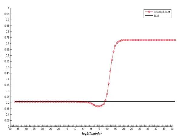
So, it is important to select a proper regularization parameter for the ELM. However, there is no general method to choose a proper or an optimal regularization parameter so far. Deng et al. (2009) have proposed a numerical heuristic method based on cross-validation to determine the regularization parameter. The specific procedure can be described as follows:

Regularization method proposed by Deng et al. (2009) Given a training set withN distinct samples,

x={(xi,yi)|xi∈Rn,yi∈Rm,i=1,2, . . . ,N}, activation function ϕ(x), and the number of hidden neuronsL

1. Randomize all the training samples and then divide them into two portion by a ratio of three to one. The portion with most training samples still serve as the training set(xtrain,ytrain). The other portion does duty for a validation set

(xval,yval).

2. Choose all values in the interval [2−50,2−49,2−48, . . . ,248,249,250] as the

regu-larization parameter, then train the regularized ELM with different regular-ization parameter and compute the corresponding output weight matrix ˆβ

with the training set.

3. Compute the outputs of the validation set with each estimated output weight matrix:

Out put(xval)=h(xval)Bˆ =h(xval)(HTH+λI)−1HTYtrain

4. Test the performance and accuracy of regularized ELM with different regular-ization parameter on the validation set. For each regularized ELM with differ-ent regularization parameter, compute the root-mean-square error (RMSE):

RMSE=

s

||Out put(xval)−Yval||2 nval

5. Choose the value as the regularization parameter which makes the corre-sponding regularized ELM perform best and minimizes the RMSE in the val-idation set.

There are two vital drawbacks of this numerical heuristic method.

• It takes a lot of time to traverse all the candidate regularization parameter. For

the interval [2−50,2−49,2−48, . . . ,248,249,250] mentioned above, we have to train

101 regularized ELMs. In real-life applications with a large amount of training data, which is in high-dimensional feature space, this method consumes such long time that it violates the purpose of ELM, which aim to shorten the training time significantly.

• In addition, it is possible that a proper regularization parameter cannot be found

and determined with such method. The figure 3.1 shows an example, in which the regularization parameter is determined by this numerical heuristic method. However, in some particular case, the regularization may locate at the exact mid-dle of the interval, for example,[230,231]. It is not likely to find this regularization

parameter, since we have not tried any other values in this interval besides 230 and 231_{, so that we cannot obtain a similar curve as in 3.1 demonstrated to find} the minimum of RMSE.

27

Chapter 4

A-optimal Design Regularization and

its Application in ELM

As it is discussed in the previous chapter, a proper or even optimal regularization parameter is necessary for controlling the weight given to the term of quadratic norm of the coefficients of the output weight matrix, relative to the minimization of the term of the quadratic norm of the output errors. So far, there has been left the open problem to evaluate the regularization parameter for balancing the these two quadratic terms. On one hand, it is insufficient to overcome the over-fitting problems of normal ELMs when the value of the regularization parameter is too small. On the other hand, it will lead to under-fitting so that we cannot approximate the data in high accuracy, when the regularization parameter is of large value.

In order to acquire an optimal regularization parameter, we apply A-optimal design regularization, proposed by Cai (2004), to determinate the regularization parameter. Before introducing the A-optimal design regularization, it is necessary to review the theory ofλ−weighted biased linear estimation.

4.1

λ

−

weighted Best Linear Estimation

For normal ELMs without any regularization, the least squares solution of the output weight matrixBaccording to Moore-Penrose generalized inverse is a type of best linear

uniform unbiased estimate (BLUUE). But now, we aim to estimate the solution of the output weight matrix by giving up the unbiasedness and keeping the set-up of a linear estimate ˆB=LY of homogeneous type, which is based on hybrid norm optimization

of type:

i minimum variance, ii minimum bias.

This type of linear estimate is nameλ−weighted homogeneously Best Linear Estimate

( Tikhonov (1963), Phillips (1962)). The regularization parameter determination is sys-tematically developed by Cai et al. (2004) using A-optimal design regularization of type:

Minimize the trace of theλ,Smodified Mean Square Error matrix (MSE):

tr(MSEλ,S(Bˆ))of the output weight matrix ˆB(λ−homBLE)to find

λopt=argtr(MSEλ,S(Bˆ)) =min

It is essential to understand the composition of the MSE matrix. Therefore, the bias vector and the bias matrix as well as of the MSE matrix with respect to the homoge-neously linear estimate ˆB=Lyof fixed effectB, which represents the real value, in the

following box. dispersion matrix D(Bˆ)=LD(Y)LT (4.1) bias vector b=E(Bˆ −B) =E(Bˆ)−B (4.2) =LE(Y)−B=−(I−LH)B bias matrix Bias=I−LH (4.3) decomposition ˆ B−B= (Bˆ −E(Bˆ)) + (E(Bˆ)−B) (4.4) =L(Y−E(Y))−(I−LH)B MSE matrix MSE(Bˆ)=E((Bˆ −B)(Bˆ −B)T) (4.5) =LD(Y)LT + (I−LH)BBT(I−LH)T

The bias vectorbis conventionally defined byE(Bˆ −B)subject to the homogeneously

linear estimate B=LY. Since the fixed effectsβis unknown in general situation, there

has been made the proposal to instead use the matrix I−LH as a matrix-valued

mea-surement of the bias. The MSE matrix MSE(Bˆ)can be decomposed into two parts:

4.1 λ−weighted Best Linear Estimation 29

• the dynamic bias productbbT

After introducing the MSE matrix, we can presentλ−homBLE with hybrid minimum

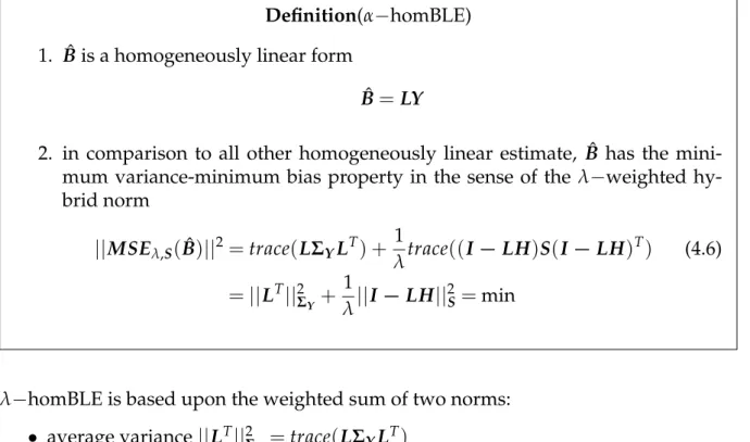
variance-minimum bias in the following definition Definition(α−homBLE)

1. ˆBis a homogeneously linear form

ˆ

B=LY

2. in comparison to all other homogeneously linear estimate, ˆB has the

mini-mum variance-minimini-mum bias property in the sense of the λ−weighted

hy-brid norm ||MSEλ,S(Bˆ)|| 2_=trace(LΣ YLT) + 1 λtrace((I−LH)S(I−LH) T_{) (4.6)} =||LT||2_Σ Y + 1 λ||I−LH|| 2 S =min

λ−homBLE is based upon the weighted sum of two norms:

• average variance||LT||2_Σ Y =trace(LΣYL T₎ • average bias 1 λ||I−LH|| 2 S =λ1trace((I−LH)S(I−LH) T₎

λ−homBLE balances the variance and the bias by factorλ, which is illustrated by the

following figure.

Figure 4.1:Balance of the variance and the bias by the weighting factorλ; source: Cai (2004)

The hybrid norm ||MSEλ,S(Bˆ)||

2 _{established the Lagrangian for ˆB as}

λ−homBLE of x.

L(L):=trace(LΣYLT) + 1

λtrace((I−LA)S(I−LA)

Then equivalent representation of the solution of normal equation is ˆ

B= (HTΣYH+λS−1)−1HTΣ_Y−1Y (4.8)

For ELMs, all training samples are equal weighted, so the weight matrix ΣY = I. In

addition, the unit matrix I is chosen as the regularization matrix S. Thus, we can

rewrite the equation (4.8) as ˆ

B= (HTH+λI−1)−1HTY (4.9)

Complemented by the dispersion matrix

D(Bˆ)=(HTH+λI)−1HTH(HTH+λI)−1 (4.10)

by the bias vector

b=E(Bˆ −B)

=−(I−(HTH+λI)−1HTH)B (4.11)

=−λ(HTH+λI)−1B

and by the MSE matrix

MSE(Bˆ) =E((Bˆ −B)(Bˆ −B)T) =D(Bˆ) +bbT

= (HTH+λI)−1HTH(HTH+λI)−1

+ [(HTH+λI)−1λI]BBT[λI(HTH+λI)−1] (4.12)

= (HTH+λI)−1[HTH+ (λI)BBT(λI)](HTH+λI)−1

4.2 A-optimal design Regularization

In order to minimize the trace of MSE matrix, the A-optimal design regularization is applied to determine the optimal regularization parameter, which optimize the the trace of MSE matrix. The regularization parameter λ follows by A-optimal design

regularization in the sense of minimizing the trace of MSE matrix (trace(MSE(Bˆ)) =

min), if and only if ˆ

λ= trace(H

TH(HTH+ ˆ

λI)−3)

BT_(HT_H+λˆ_I)−2_HT_H(HT_H+λˆ_I)−1_B (4.13) The proof og the formula of type 4.13 will be given in the appendix. Moreover, we will interpreted how the A-optimal design regularization is applied in improving the performance of ELMs. We will discuss in two different cases.

4.2 A-optimal design Regularization 31

1), ELMs with Single Output

For the cases, where there is only a single output neuron in the output layer, the output of an ELM is a single numerical consequence, for example, regression problems and binary classifications. In such cases, the number of output neurons ism=1, therefore,

the output weight is a L×1 vector.

For ELMs with single output, A-optimal design regularization can be directly used to determine the regularization parameter.

2), ELMs with Multiple Outputs

When we use ELMs to classify images into m classes in multi-class classification, the ELMs will have m output neurons. The output of the ELM is a vector rather than a single number. The expected output vector of the m output neurons is yi= [0, . . . ,0,

p

1,0, . . . ,0], if the original class label is p. Specifically, only the pthelement ofyi= [yi1,yi2, . . . ,yim]T is one, while the rest of the elements are set to zero.

In such cases, the A-optimal design regularization cannot be applied to compute the regularization parameter for the ELMs directly, since the denominator in the right hand of equation (4.13) is a matrix, however, the numerator is rather a number.

In order to apply A-optimal design regularization in ELMs for multiple outputs, we have to go back to equation (3.24).

ˆ

B= (HTH+λI)−1HTY

In such equation demonstrated above, we have the outputY as aN×mmatrix, when there are Ndistinct training samples andmoutput neurons. As it is already discussed in chapter 3, when the number of the hidden neurons in ELMs counts L, the output weight is thus a L×m matrix. According to Cai (2004), the equation (3.24) can be decomposed into the following equations.

ˆ β1= (HTH+λ1I)−1HTy1 ˆ β2= (HTH+λ2I)−1HTy2 ... (4.14) ˆ βm= (HTH+λmI)−1HTym

The ith column of the output matrix and the output weight is corresponding yi =

[y1i,y2i, . . . ,yNi]and ˆβi= [βˆ1i, ˆβ2i, . . . , ˆβLi], fori=1,2, . . . ,m. We can determine the regu-larization parameter λiand the corresponding column ˆβi of the output weight matrix by the A-optimal design regularization, fori=1,2, . . . ,m.

33

Chapter 5

Case Studies: Application of A-optimal

Design Regularization in Extreme

Learning Machine

In order to inspect whether A-optimal design regularization helps to improve the per-formance of ELMs or not, we implement three case studies to research ELMs with A-optimal design regularization and compare the performance of regularized ELMs with the original ones.

5.1 Approximation of Sine Function

The first case study is an artificial simulation about approximating sine function y=

f(x) =sin(x) by both regularized and original ELMs. We will approximate the sine

function in two different situations.

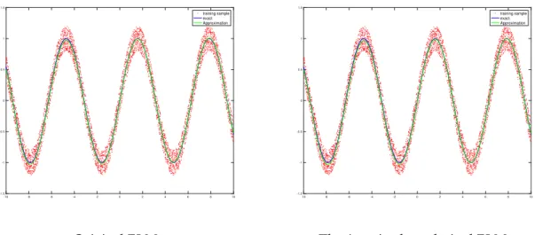
• In the first situation, there is no outliers in the training set. The training set is

cre-ated by 5000 distinct samples of sine function, which are uniformly and randomly distributed on the interval (−10,10). In addition, random noise distributed on

the interval [−0.2,0.2] will be added to all the training samples. Similarly, 5000

distinct samples are randomly chosen to generate the testing set, while all the testing samples still remain noise-free.

• In the second situation, 100 outliers randomly distributed in the range of[−2,2]

will be added into the training set. Moreover, we choose other 4900 distinct sam-ples with the same method as used in the first situation to constitute the training set. As same as the first situation, the testing set is composed of 5000 noise-free distinct samples of the sine function.

In the following table, the information of training and testing data in both situation is listed in detail.

Table 5.1:Data Information for Approximation of the Sine Function

Training Set Testing Set

without outliers distinct samples outliers noisy distinct samples noisy_{5000 0 yes 5000 no} with outliers distinct samples outliers noisy distinct samples noisy_{4900 100 yes 5000 no}

In both situations, we train the original ELM and the A-optimal design regularized one with the training set to approximate the sine function respectively. Moreover, the per-formance of both algorithms will be evaluated on the corresponding testing set in each situation. Specifically, RMSE for the testing set of both algorithms will be computed and compared in each situation. The following table shows us the comparison of the RMSE between both algorithms.

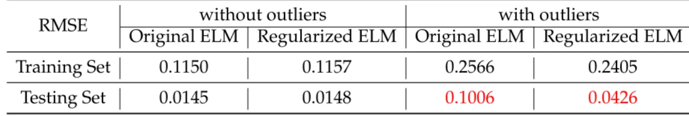
Table 5.2:Comparison of RMSE of the original ELM and the ELM with A-optimal design regularization in both situations

RMSE _{Original ELM Regularized ELM Original ELM Regularized ELM}without outliers with outliers

Training Set 0.1150 0.1157 0.2566 0.2405

Testing Set 0.0145 0.0148 0.1006 0.0426

From the table above, it is obvious that there is no significant difference between both algorithms, when there is no outliers. Both algorithms have good performances and the RMSE for the testing set of both algorithms are very low. But for the situation, where there is outliers in the training set, the ELM with A-optimal design regulariza-tion performs much better than the original one. It implies that the performance of the original ELM is seriously influenced by the outliers. While for the A-optimal regular-ized ELM, honestly, the performance is more or less affected by the outliers as well. However, the RMSE for the testing set is still very low. In other words, the the ELM with A-optimal design regularization is much more robust against the outliers than the original ELM, i