Borrower Characteristics and Mortgage Choices

(1)

Borrower Characteristics and Mortgage Choices

∗

Mardi Dungey

∗+&

, Graeme Wells

∗&

and Maria Yanotti

∗

University of Tasmania

+ CFAP, University of Cambridge

& CAMA, Australian National University

22 November 2012

Preliminary: Do not cite without permission

Abstract

Empirical evidence on the role of borrower characteristics in mortgage product choice is mixed. Using uniquely detailed data on over 600,000 mortgage applications we show that borrower characteristics play a significant role in choosing between adjustable rate mortgages and more complex products. Whilst this indicates that mortgage markets are incomplete, the results are consistent with product choice which reduces household exposure to income, wealth and mobility risk. As the sample covers the period 2003-2009 we exploit the change in supply conditions arising from the global financial crisis to examine the effect of the increased cost to the bank of holding risky loans on their balance sheet. The observed changes in the effects of borrower characteristics on household mortgage product choice are consistent with the bank responding by changing the terms of the mortgage or transferring income and mobility risk to the mortgage applicant.

JEL Categories: G21, G01

Keywords: mortgages, household finance

∗_{We acknowledge funding support from Australian Research Council grant DP120100842}

and research assistance from Sharon Raymond. Author contacts: Mardi.Dungey@utas.edu.au, Graeme.Wells@utas.edu.au; Maria.Yanotti@utas.edu.au (corresponding author).

(2)

1 Introduction

In a complete mortgage market informed lenders offer informed borrowers customized contracts (with a vector of ‘price’ characteristics including loan-to-value ratio, term to maturity, interest rate, and interest-rate flexibility) which fully price risk, and customers self-select the appropriate product. In this environment, observable ‘prices’ determine the choice of mortgage product; borrower characteristics have no additional explanatory content.

As will be detailed in Section 2, existing literature provides mixed evidence on the role of borrower characteristics in mortgage choice. Mixed results could emerge for a number of reasons. In some studies, only a limited range of borrower characteristics is considered, biasing the results against finding any role for characteristics. In other studies market structure may play a role – for example, lenders may have little incentive to fully price risk because of public subsidies to risk-taking. This paper is the first to empirically investigate household choice between a variety of mortgage products with the inclusion of a full range of borrower characteristics. It is also the first to try and pin down the role played by borrower characteristics in terms of supply and demand effects.

This paper has two objectives. The first is to investigate the extent to which borrower characteristics have a role in determining mortgage product choice, using a database of 600,000 mortgage applications to a major Australian bank from 2003-2009. These data include all information provided to the bank at mortgage origination, with the exception of the identity of the borrower. We find that borrower characteristics play a role in mortgage choice.

Knowing how borrower characteristics play a role is important because, as Miles (2004, 2005) emphasizes, incompleteness in mortgage markets may be symptomatic of inefficiency. Although our findings indicate market incompleteness, they do not neces-sarily imply market inefficiency because, as shown later in the paper, mortgage contracts emerging from the interaction between lenders and borrowers appear to exploit informa-tion embedded in characteristics to reduce exposure to risks faced by borrowers.

Our second objective is to determine which side of the market makes most use of this information. One possibility is that well-informed borrowers know the risks they face, and make appropriate choices as to the type of mortgage product to purchase. Our prior is that this is unlikely, given recent evidence as to the financial literacy of households (Lusardi and Mitchell 2007; ANZ 2008; Bateman et al. 2012; Campbell et al. 2009). An alternative is that lenders set ‘prices’ which induce borrowers to choose risk-reducing mortgage products.

(3)

this issue, because supply conditions faced by Australian banks changed. A distinctive feature of the Australian market is that the large banks have not dispersed default risk on mortgages by securitizing. The large banks hold almost all their mortgage risk on their balance sheets. Before the financial crisis, the biggest four banks had securitized 5% of their funding liabilities; immediately after the crisis, securitization fell to 1%.

The major change in supply conditions is not that there was a marked change in securitization but that, after 2007, the cost of holding mortgage risk on the banks’ balance sheet increased rapidly. One indicator of this change is the spread on credit default swaps with which banks insure the default risk of mortgages on their balance sheet. In the five years prior to 2007, this spread averaged 20 basis points; after 2007 the spread rose rapidly, reaching more than 180 basis points towards the end of our sample period.

We hypothesize that this change in supply conditions motivated banks to more fully exploit information provided in mortgage applications, offering contracts with ‘prices’ inducing customers to take products which, given characteristics observable by the bank, reduced default risk. Results reported below are mixed — for some customers, prices are set which induce customers to take contracts which reduce income risk; in other cases, it appears that the bank shifts risk to mortgage applicants.

The paper proceeds as follows. Section 2 provides an overview of the potential de-terminants of household mortgage choice. Section 3 describes the Australian mortgage market and the data set. The empirical methodology is given in Section 4 and Section 5 presents the results. Section 6 concludes.

2 Risks and Mortgage Choice

Householders face a number of risks which reflect their own characteristics in assessing lifetime financial decisions; Campbell (2006); Campbell and Cocco (2003). Income risk describes the potential volatility of household income which may arise through periods of unemployment or changing real wages via inflation, or potential lifetime income growth through increased skills. Wealth risk includes the potential for capital gain or loss via fluctuations in house prices, the potential for transfer of wealth from creditor to debtor via the effects of inflation on nominal contracts, and the barriers to entry which may be created by wealth constraints such as minimum downpayment requirements in order to enter the housing market. Households do not necessarily consume services of only one house during their ‘lifetime’. For a variety of reasons related to employment, changing family structure, taxation benefits or changing circumstance they may find it desirable to change home. In these circumstances remaining an owner-occupier involves mortgage costs, such as reapplication fees, mortgage break fees, selling and buying costs and

(4)

gov-ernment taxation. In the literature, the costs of renegotiating the mortgage expose the householder to mobility risk.

The literature on mortgage choice has been dominated by investigations of the choice between traditional ARM and FRM mortgages. An ARM mortgage is usually a long term mortgage with the variable rate determined by the financial institution, or subject to periodic adjustment in line with current market conditions. FRM mortgages are typically long term fixed rate contracts, where the mortgagee pays a cost to break the contract. The empirical literature has generally concentrated on US based results, where FRM contracts have a large share of the market.

There have been important innovations in the household mortgage market in the past decade. The most prominently investigated is the increased securitization of mortgages and other consumer debt, to which is widely attributed the rise of lending to subprime borrowers and ultimately the trigger for the global financial crisis.1 _{The period has}

also seen important innovations in product offerings. Increasing market share in many economies has been captured by products which reduce the initial payment burden for the consumer, but retain the longer term mortgage risks with the consumer, not the financial institution. Such products include honeymoon or teaser mortgages, which offer a discounted introductory interest rate, contracts with periodically reset fixed interest rates, and equity withdrawal mortgages.

While the choice between fixed rate mortgages (FRM) and adjustable rate mortgages (ARM) has been most commonly investigated in the existing literature, Amromin et al (2011) introduced a new category of complex mortgages (CM) to denote the increasing array of mortgage products ranging between ARM and FRM products. This paper is the first to empirically investigate household choice between CM and ARM mortgage products with the inclusion of a full range of borrower characteristics. Amromin et al (2011) examine choice between ARM, CM and FRM in the US but have only income and geographical proxies available for borrower characteristics. Sa-Aadu and Sirmans (1995) investigate a range of different mortgage options which are distinguished only by frequency of interest rate adjustment and term.

The introduction of CM contracts means that consumers have a greater range of options to fit their circumstances. It additionally means that a number of hypotheses developed for the choice of ARM over FRM mortgages should be re-examined to ascertain whether a nuanced examination of these products more clearly identifies the hypothesized relationships between household characteristics and mortgage product choice.

We expect that consumers facing income risks will take a product which reduces the

1_{For example in the testimony of Alan Greenspan to Financial Crisis Inquiry Commission, April 7,}

(5)

variability of their payments. Thus, a FRM would be preferred to an ARM. Tests of this proposition have been attempted in the literature using proxies such as the pres-ence of children, age, income levels and growth, education, self-employment or public employee, and income volatility estimated using a Mincer equation – see Brueckner and Follain (1988), Dhillon et al (1987), Sa-Aadu and Sirmans (1995), Leece (2000), Paiella and Pozzolo (2007), Colibaly and Li (2009) – with little success in obtaining significant relationships.

The potential for future household income growth, which would reduce the importance of mortgage payments in the household budget, is expected to increase the propensity of households to take ARMs over FRMs. But again the literature has had mixed success proxying for this effect; age dummies in Brueckner and Follain (1988) and income in Paiella and Pozzolo (2007) show little evidence although income growth data in Sa-Aadu and Sirmans (1995) finds significant impact in the expected direction.

Likewise, borrowers who expect to make capital gains on housing (usually represented empirically by past housing price inflation) will also be willing to take on a product where they bear more of the risk. In Dhillon et al (1987) this means the borrower will be more willing to take an ARM than FRM, but when faced with the opportunity of a CM product and initial wealth constraints this could also mean that a buyer will be willing to take the risk of exposure to the housing market and take a CM. So despite the evidence that ARM is preferred to FRM in expectation of wealth creation, the sign is not clearly determined when CM products are also available. Amromin et al (2011) discover that when house price inflation is expected borrowers prefer CM products.

First-time buyers are expected to be more wealth constrained than repeat buyers, and Ortalo-Magne and Rady (2006) suggest they have a critical impact on the state of the housing market itself. Wealth constraints are expected to influence their choices away from ARM products; however, the use of dummies for this category has failed to show significant evidence in Dhillon et al (1987) and Brueckner and Follain (1988). On the other hand, CM products are designed to reduce early period payments and we would expect that a first home buyer would be more likely to select a CM loan due to a downpayment constraint.

Mobility risk should induce households to purchase products with the least penalty for moving. Mortgage products with fixed rates in some jurisdictions fully amortize the cost to the lender of prepayment, imposing a substantial penalty for refinancing; in the US borrowers select up-front the ‘points’ they are willing to pay to obtain more flexibility in refinancing or moving the contract. Dhillon et al (1987), Brueckner and Follain (1988), Sa-Aadu and Sirmans (1995) all confirm the positive impact of mobility on choice of ARM products.

(6)

The literature on mortgage choice is currently undergoing a strong resurgence, partly due to interest in the role of securitized mortgages in the propagation of the global financial crisis and the subsequent exploration of greatly improved data resources. Many past studies have been severely limited in the data available; Dhillion et al (1987) had only 78 observations, Brueckner and Follain (1988) have 475 observations, Brueckner (1994) has 418 observations and each of them include survey data, interpolated data and generated proxies and draw from relatively constrained geographic areas. More recently larger data sets have emerged. Paiella and Pozzolo (2007) have 28,000 observations for Italy compiled from a representative survey. However, the most convincing new evidence is emerging from datasets compiled from financial institutions or regulatory authorities’ collections of data - including 600,000 observations in Berndt et al (2010), 780,000 in Fortowsky et al (2011) and 10 million observations in Amromin et al (2011). The dataset used in the current paper is distinguished by the wealth of detail generated by the bank in the course of processing applications.

Despite the lack of consensus over the effects of individual household characteristics on mortgage choice, there are consistent results regarding the cost of mortgage products. Increased cost of a FRM mortgage relative to an ARM mortgage will tend to favour choice of an ARM. This has been found in the case of bank fees, repayment penalties and regular repayments. The sign on arguably the most important cost variable, the interest rate differential, is positive in empirical studies. When a more flexible interest rate product (where the ranking from most flexible to least is ARM, CM, FRM) offers a lower interest rate, households may be attracted to that product. However, this may not be the case if the relatively low current flexible interest rate is expected to rise. Some papers have observed that even at times when FRM interest rates are high borrowers may still prefer this type of product. To date Dhillon et al (1987), Brueckner and Follain (1988) and Paiella and Pozzolo (2007) support a positive effect for ARM choice over FRM when ARM interest rates are relatively lower. Other studies such as Amromin et al (2011) do not include these cost variables.

This paper furthers the investigation of household mortgage choice using a unique mortgage application database containing a much larger bank-validated borrower charac-teristic data set than has previously been available. The data include all the information solicited from the customer, and validated by the bank, and thus provides a significant improvement in data quality associating borrower characteristics with observed product choice. The data refers to mortgage applications in Australia, and the following section provides contextual background to the Australian mortgage market and the database.

(7)

3 Background and Data

The Australian banking industry has a high degree of concentration, with the five largest banks having more than 60 per cent of owner-occupied loan approvals. Smaller banks have around 20 per cent market share, credit unions and building societies less than 10 per cent, and wholesale mortgage originators less than 10 per cent (Davies, 2009). The share of total housing credit funded by securitization rose from 10 per cent in 2000 to more than 20 per cent in 2007, at which point issuance of residential mortgage backed securities (RMBS) fell sharply with the onset of the global financial crisis. Almost all this increase reflected the use of securitization as a funding vehicle for mortgage originators, credit unions and smaller banks to access competitive funding. Large banks made little use of securitisation. In 2007 securitisation comprised 5% of funding liabilities; in 2010 this had fallen to 1% (Debelle, 2008, 2009; Brown et al. 2010).

As in many countries, the Australian housing market is impacted by taxes and sub-sidies. Capital gains tax is not generally payable on owner-occupied homes, and the consumption services provided by owner-occupation are not taxable. While mortgage interest payable by owner-occupiers is not tax deductible, owners of dwellings purchased for investment purposes receive a deduction against wage and salary income for all asso-ciated expenses. Tax losses made in this way are not capped. Loans for owner-occupied housing comprise two third of banks’ outstanding housing loans, and this proportion has shown very little variation in the last decade which includes our sample period.2

There is a variety of grants and tax concessions offered by the federal government and the states to first home buyers (Dungey et al. 2011). These concessions are directed towards a social objective of encouraging home ownership, and were used as an instrument of macroeconomic stabilization towards the end of 2008 in response to the global financial crisis.

The data used in this study are bank-originated mortgages issued to applicants for owner-occupied housing including applications for the refinancing of existing home loans, for the period of January 2003 to May 2009. In the period up to 2007 mortgage brokers provided an increasing proportion of housing loan originations via referral to financial institutions. Banks pay commissions to third party originators in ways which potentially bias the characteristics of mortgages issued; for this reason, these applicants were excluded from the analysis.

The predominant mortgage product in Australia is a standard ARM product, which is a credit foncier loan written for terms of up to 40 years, with the interest rate adjustable at the discretion of the bank. A FRM such as commonly described in the international

(8)

literature with a rate fixed for a very long term is not available; instead a loan with an interest rate fixed for an initial period (usually between 3 to 5 years) is offered, after which terms are renegotiated. Under renegotiation the options include conversion to an ARM or to a second FRM. Full cost recovery fees apply to customers wishing to exit fixed rate contracts prior to the expiration of the fixed rate period if market interest rates fall below the agreed rate. In the parlance of the existing literature, this is a CM product.

A range of other CM products have arisen in the last decade, including reverse mort-gages, honeymoon mortmort-gages, interest-only loans, shared-equity loans, low-doc loans for borrowers who self-report their financial position and forms of non-conforming loans for borrowers not meeting standard lending criteria. However, Debelle (2010), reported that low-doc loans never comprised more than 10 per cent of housing loan approvals, and non-conforming loans never exceeded 2 per cent of the total in data up to 2009.

Under the Basel capital adequacy rules operative during the sample period, residential mortgage loans qualified for a concessional risk weight of 50 per cent if the loan-to-value ratio was less than 80 per cent, or 60 per cent for a low-doc loan. Loans which did not meet these criteria only qualified if they were fully insured with an acceptable lenders mortgage insurer. For the large banks, the average loan-to-value ratio (LVR) was 67 per cent in September 2006 (APRA, 2008); this ratio is representative for the whole sample period.

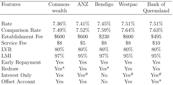
Tables 1 and 2 give a snapshot of the Australian environment. The tables report char-acteristics of standard products offered by the 5 representative banks mortgage providers (4 of the major banks) from the literature those institutions advertised for their potential customers in the first fortnight of October 2010. Table 1 describes the characteristics of the ARM (also known as Standard Variable Rate loans), where it is clear that there is a great deal of uniformity in the fees, the loan-to-value ratio offered without mortgage in-surance (the LMI refers to the loan-to-value ratio when mortgage inin-surance is purchased) and the options for other features of the loan. Table 2 gives similar information for CM loans where the interest rate is fixed for an initial period. The top row gives the range of fixed term periods offered. Note that the option of early repayment is provided for only a part of the total loan, and a number of more flexible features of the ARM loan are either entirely or partially absent.

Data used in the present analysis are drawn from a period in which Australian house prices grew rapidly, rising by 63 per cent in nominal terms between March 2003 and December 2009. Rising house prices were supported by strong growth in bank lending, with annual growth in bank-provided housing finance averaging 14.2 per cent over the same period. Banks adopted the practice of setting rates for standard ARMs with a fixed margin over the Reserve Bank’s target for the cash rate while, until the onset of the

(9)

subprime crisis in 2007, the three year FRM rate was set with reference to the three-year government bond rate. As a result, the relationship between these two lending rates closely reflect shifts in the Australian yield curve. The national unemployment rate was 6 per cent at the beginning of the sample period, falling steadily to 4.1 per cent in April 2008 before rising to a post-GFC peak of 5.8 percent in August 2009.

The data set comprises 617,868 home loan applications for the January 2003 to May 2009 for seven States or Territories of Australia.3 _{The data includes ARMs and CMs,}

with 38 percent of the total being CM. In the Australian context there are no FRM loans which are fixed for a full term. (These results compare with the dataset of Amromin et al (2011) which consists of 70 percent FRM, 17 percent CM and 13 percent ARM -clearly the structure of the markets is quite different, see also Ellis, 2006). Data cleaning reduced the usable observations to 607585 observations.4

Although the data have both a time and cross section dimension they do not constitute a panel - they are a record of mortgage application in which repeat applications, if any, by the same household cannot be identified. Thus the approach should be considered as a large pool of data with appropriate controls for the time-varying economic conditions which prevail at the point of mortgage application.

Tables 3 and 4 lay out the characteristics of the dataset in the period we label pre-GFC, from March 2003 to August 2008. Sensitivity analysis shows that these characteristics are not materially affected by choosing alternative earlier dates for the beginning of the crisis, so we adopt the convention in much of the crisis literature of dating the crisis period from September 2008, the month when Lehman Bros declared bankruptcy and the subsequent chain of collapses and rescues detailed elsewhere.

Table 3 shows the mortgage cost variables in the database. The average size of the ARM contract is just over $150,000 and the CM is $121,000. However, some very large contracts skew this picture, with the median ARM contract just under $131,000 and the median CM just over $104,000. For this reason we concentrate on reporting the median results in the tables. The median term for each mortgage type is the same at 30 years, noting that we have no information on the term of any honeymoon arrangements or

3_{These are Australian Capital Territory (ACT), New South Wales (NSW), Queensland (QLD), South}

Australia (SA), Tasmania (TAS), Victoria (VIC) and Western Australia (WA). The Northern Territory (NT) is excluded. The majority of applications are recorded for NSW, QLD and VIC, consistent with the population distribution in Australia.

4_{Deleted observations comprise (number deleted = 10283): Missing mortgage code (855), applications}

recording real gross or net monthly income of less than $10 (9141), applications recording monthly income of less than $50 (25); applications with scheduled repayments or implied rent of zero (146); applications with interest rate of zero (10); applications where the age of applicant was less than 17 years (17) or missing (5); and applications where the time at current address exceeded the applicants age (84).

(10)

how long an initial fixed rate period may be in the dataset. The median initial monthly repayment on an ARM mortgage, given that it is larger than a CM, is also higher. The median ARM initial monthly repayment is $883 while for CM it is $680; the ratio of median ARM mortgage size to CM mortgage size is 1.25, but the ratio of initial monthly repayment on the ARM to initial monthly repayment on CM is 1.30 - indicating the extent of extra security CM borrowers are achieving in the early part of their loans.

The interest rate at origination for an ARM is slightly higher than for a CM; a difference of about 12 basis points between the median rates for each loan type. Bank fees are only $12 higher for the ARM applicant than the CM. The loan-to-value ratio is similar for both contract types, at 65.64 percent for CM borrowers and 64.40 percent for ARM borrowers, which is similar to the rate reported by APRA of 67 percent in September 2006. (ARM borrowers’ median house valuation was $226,244, while CM median house valuations were around $30,000 lower at $197,468.)

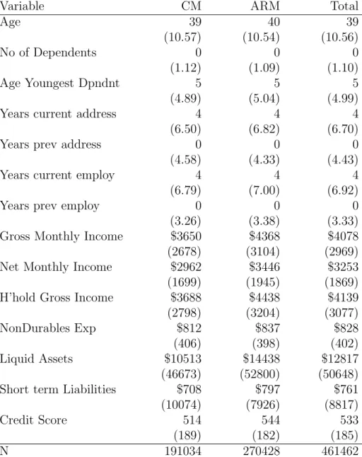
Table 4 presents median household characteristics of the borrowers for each type of contract. The median borrower for a CM is 39 years old, and 40 years old for an ARM. The median gross monthly income for a CM applicant is $3650 ($43800 per annum) and for an ARM applicant $4368 ($52416 per annum), and the primary applicant accounts for almost all this income - the median household income for a CM applicant is less than $500 per annum higher, and for an ARM applicant less than $900 per annum higher. The credit scores of the ARM applicants are slightly higher than those of the CM applicants.5 The typical applicant for either loan type has no children, but the median age of the youngest dependant for those with children is 5 years old. They have spent about 4 years in their current employment and the same time living at their current address; however the time in current employment and time at current address is not perfectly correlated across the database.

4 Empirical Specification

At time t, household i makes a decision to choose the mortgage product, y∗_i,t which best matches its risk profile given mortgage costs, the economic and credit market conditions

5_{First-time buyers typically take a slightly larger loan than the repeat purchasers, but for a lower}

valued housing stock, and have a correspondingly higher initial repayment and a higher loan to value ratio. However, they face a slightly lower interest rate, reflecting greater likelihood of selecting a CM rather than ARM product. A first-time borrower is about 10 years younger than a repeat borrower, and has lived slightly less time at their previous address, had a shorter employment history and younger children. Their income is approximately 15 percent lower than the repeat buyer, and surplus wealth considerably lower. They also have lower credit scores, and expenditure on non-durables.

(11)

prevailing, and household characteristics. That is

y_i,t∗ =αt+βXi,t +δZi,t+γWt+εi,t

where Xi,t represents the mortgage cost variables faced by individual i at time t, Wt are the macroeconomic and credit market conditions prevailing at time t, and Zi,t are individual household characteristics – these are observed at one particular timet for any individual household. The residual εi,t is assumed i.i.d normal. Note that estimation here proceeds as a pooled regression, taking into account t, the time of application as a component of the explanatory variables.

However, there is not a continuum of mortgage products available, so that the ob-served behavior is the choice of either an ARM or CM product. Consequently, define the dichotomous variable yi,t as

yi,t =

1 if borrower i chooses an ARM at timet

0 if borrower i chooses a CM at time t

We are then interested in the probability of choosing an ARM which can be expressed as a probit such as:

P(yi,t = 1|X, Z, W) = Φ(αbt+βXb i,t+δZb i,t+bγWt)

where Φ(.) is the cumulative distribution of a standardized normal distribution.

An important explanatory variable in the existing literature is the interest rate differ-ential between alternative mortgages available to the householder at the time of applica-tion. This is an unobservable variable, as only the interest rate of the chosen contract is recorded, and the comparable alternative is not. This can be addressed in a number of alternative ways.

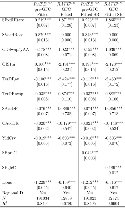
First, we calculate the monthly average interest rate for each mortgage contract (ARM, CM) and use those averages to compute the interest rate differential between types. This simple approach will be valid if the lender offers similar contracts to all customers for a period. Given that we have data provided by a single lender this may be a reasonable approximation. A second approach is to estimate the rate differential following Brueckner and Follain (1988), who suggest using the differential between fitted values of

RAT E_i,tCM = BCV_i,tC +uC_i,t

RAT E_i,tARM = BAV_i,tA+uA_i,t

where VC_, _VA _{are vectors containing the determinants of the interest rates on CM and} ARM products respectively, and contain variables belonging to the set {X, W, Z}, BC

(12)

and BA _{are corresponding loading vectors and the residuals} _uC _and _uA _{are i.i.d normal.} The predicted interest rate differential is then formed as the difference between the fitted values

RAT EDIF F api,t =BcCV_i,tC−BcAV_i,tA.

Three different alternatives are then available for use in the probit estimation. These are the simple differences between the average observed monthly rates as described above, denoted here as RtDif f; second, the difference between the estimated interest rates replacing all values in the dataset with their predicted values denoted asRAT EDIF F ap; and finally, recognizing that this last form suffers from selectivity bias, a selectivity bias corrected measure of the predicted values (using the inverse Mills ratio) which we denote

RAT EDIF F apsb. These are augmented by dummies for the state of loan origination,

and the explanatory variables in VA_and _VC _{include measures of interest rates at varying} maturities. Tables 5 and 6 present the fitted regressions for the interest rates.

5 Empirical Results

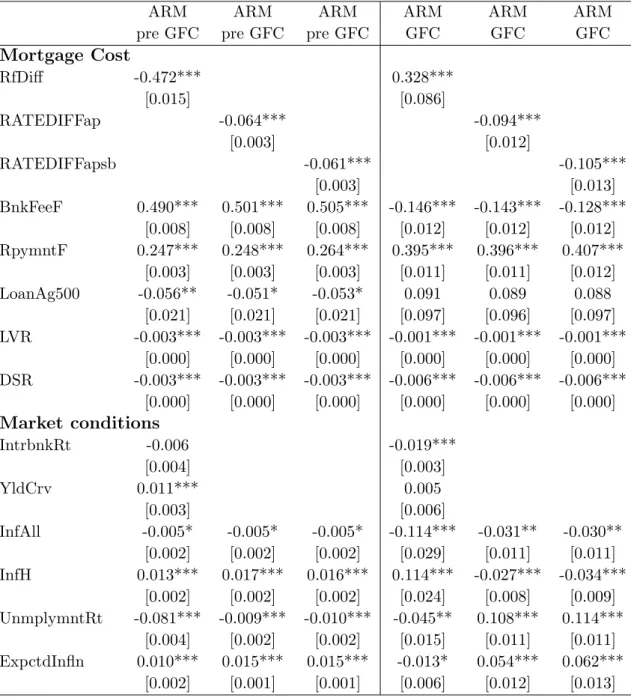
Table 7 presents the estimation results for the marginal effects of variables contained in X, W or Z for each of the pre-GFC period, and the GFC period using the three different potential specifications of the interest rate differential. The cost variables, X, are represented by the interest differential between CM and ARM mortgages, bank fees, the monthly mortgage repayment, a dummy to represent loans of over $500,000, the loan-to-value ratio (LVR) and debt service ratio (DSR). Exact definitions of the cost variable names are given in Appendix Table A1.

The market conditions variables, W, include the prevailing money market rate, the slope of the Commonwealth Treasury yield curve between the 10 year and 90 day bill rate, the consumer price inflation rate, the house price inflation rate, the consumer’s expected inflation rate derived from survey information and the national unemployment rate.6 To match these data to the dates in the database we use the corresponding quarterly housing and consumer price inflation rates as well as expected inflation rate. Monthly data include the unemployment rate and a monthly measure of the prevailing yield curve between the 10 year Australian Government bond and 90 day bill rate. A mortgage application processed on any day in the first month of 2003Q1, for instance, is matched to the relevant monthly and quarterly data. Definitions and sources for the market condition variables are given in Appendix Table A2.

6_{We experimented with State and Territory level unemployment rates, inflation rates and housing}

price inflation but this level of disaggregation did not provide further information than the simple national levels for each indicator.

(13)

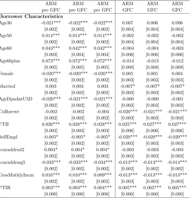
In terms of borrower characteristics, Z, we examine the effects of borrower age (both as a level and as a categorical variable), gender, marital status, whether there is a co-borrower, the number and age of dependent children, whether the borrower is a first home buyer or self-employed, occupation categories, how long the borrower has spent with their current and previous employer, how long they have spent at their current and previous address, monthly income, net wealth at time of application and geographical location. We also include variables to proxy for financial literacy such as the time the borrower has been a client of the bank, the number of credit facilities and credit accounts the borrower has, and a dummy variable to indicate whether the borrower holds shares. Variable names for borrower characteristics are defined in Table A3.

The average marginal effects for continuous variables represent the average impact of a 1 unit change in the variable, and for choice variables these are given as a change from status 0 to status 1 (e.g. unmarried to married). The baseline applicant is a 40 year old single salary-earning professional male without a co-applicant, with no dependents, who is not a first-time homebuyer.

5.1 Prior to the GFC: mortgage choice

The importance of the alternative specifications of the interest rate differential variable is immediately obvious in the pre-GFC period results in Table 5. The predicted interest rate differential approach, which we prefer, is reported in columns (2) and (3) and shows that an increase in the interest rate for a CM contract over an ARM results in a statis-tically significant dencrease in the probability of choosing an ARM mortgage. While the predicted interest rate differentials show a markedly smaller effect for a change in the interest rate differential than the observed variables, the selectivity bias correction makes relatively little difference to the marginal effect of this variable. This is consistent with the existing literature.

The differences in the marginal probabilities of other explanatory variables in the three columns for interest rate differential choices are rather small. In general, the effects are essentially the same, unless specifically pointed out in what follows.

Bank fees and the scheduled repayment amount are significant in increasing the prob-ability of an ARM. Increased repayments increase the probprob-ability of choosing an ARM and, as servicing risks increase through higher loan-to-value ratios and debt servicing ratios, households are less likely to choose an ARM over a CM. As these data are taken from the final loan approval document, this suggests that those who can afford the higher loan repayments are more likely to select the ARM contract. However, there is a thresh-old effect at work. In addition to the positive marginal effect of a larger loan repayment

(14)

reported in the results, loans of greater than $500,000 attract a reduced marginal proba-bility of selecting an ARM, of about one-tenth the size of the repayment effect. This fits with the different types of CM available; honeymoon packages are aimed at liquidity con-strained, wealth constrained and typically smaller loan borrowers, but other packages are aimed at wealthier individuals less likely to be constrained. It also fits with the analysis of the CM market in Amromin et al (2011) who find that CMs are taken by households requiring jumbo loans (that is, greater than the size of Fannie Mae and Freddie Mac conforming loans). This is worthy of further investigation.

The results show that when interbank interest rates are high, households are less likely to choose an ARM, potentially reflecting the fact that they feel that future interest rates will fall; this reflects a relatively sophisticated view of the market where participants recognize the (potentially slow) mean-reverting nature of interest rates as expressed in the very high persistence of interest rate data. This is similarly reflected in the market expectations of inflation reflected in the yield curve and in the average household inflation expectations as reported via survey data. Higher inflation expectations slightly raise the probability of an ARM product.

When current inflation is higher the results suggest a slight preference away from ARM products, however, this economic effect is very small – a rise in the quarterly inflation rate from 0.495 percent to 1.495 percent represents a tripling of the annual rate (from 1.9 percent to 5.9 percent ) but the implied decrease in probability of selecting an ARM mortgage is only 2 percent. In the light of such a stark and sudden increase in the actual inflation rate this effect is economically unimportant. When house price inflation is higher, households are keen to take on the risk of capital gain and are more willing to take on an ARM product, although as with the inflation effect this is not a particularly large economic effect, indicating that potential capital gain is a relatively small component of the drivers of owner-occupier mortgage choice. Consistent with the existing literature and theory, when income risk is higher, as represented by the unemployment rate, households are more likely to prefer CM products with stable payments.

5.1.1 Borrower Characteristics

Older applicants are more likely to choose an ARM, while those under 30 are much less likely to choose an ARM than the benchmark 40 year old applicant. Female applicants are less likely to choose an ARM product, which is consistent with the literature on greater female risk aversion and potentially lower financial literacy. In other work, we have shown that the bank does not discriminate between male and females in offering products, but that characteristics such as lower average income and education and higher numbers of dependents generally explain the lower average level of mortgage taken out

(15)

by female applicants.

Despite potentially higher risk aversion married applicants or applicants with co-borrowers do not show any statistically significant change in their probability of taking an ARM than the single benchmark applicant, however, the presence of young depen-dent children decreases the probability of selecting an ARM product. This reflects the repayment risk facing the household in terms of committed expenditures associated with children.

Despite these effects, first-time borrowers are shown to marginally prefer ARM prod-ucts over the CM. This needs to be seen in context of the benchmark who is a relatively high income, older male who chooses a CM product. The first-time home owner has lower income, has less work experience and makes a lower downpayment. Finally, income risk, as represented by self employment status, has the expected sign of reducing the probability of choosing an ARM.

The results presented here are a powerful validation of the theoretically expected signs of borrower characteristics on mortgage choice. For the first time a relatively complete set of borrower characteristics has been available to examine mortgage product choice. This database has high quality income and household characteristic data and has not had to rely on imputed or survey data to describe the household. Nor, in the Australian market, are there institutional arrangements which interfere with our observation of the risk allocation between household and financial institution in mortgage transactions. The direct consequence has been that we are able to show that as anticipated; income risk increases the probability that the household will choose a product which reduces its exposure to payment variability, at least in the first part of the contract; wealth risk leads to consumers choosing products which help alleviate their initial difficulties in meeting downpayment requirements and that mobility risk, proxied through job tenure, age and income, leads households to choose more flexible ARM products. The CM products help households manage their income and wealth risk, but also allow households to enter the housing market when they believe that potential rising house prices and rising inflation will result in a real wealth transfer from creditors to debtors.

Further insight into the role played by borrower characteristics can be obtained by comparing these results with estimates from the GFC sample. As detailed earlier, banks and borrowers faced higher risks after 2008. Banks responded to higher default risk on new loans by changing the terms on which they were offered — the loan to valuation ratio on new loans fell, for instance. The efficient market response would be for the equilibrium to be such that mortgages are offered on terms which induce relatively low-risk borrowers to take ARMs. That is, controlling for GFC values of market ‘cost’ variables, borrowers offered ‘average’ terms who are low risk relative to the basecase borrower will be more

(16)

likely to choose an ARM. Results reported in the following section suggest that this is, in fact, the case.

5.2 The aftermath of the GFC and mortgage choice:

The final three columns of Table 5 give the corresponding results for the marginal effects of the mortgage cost variables, market conditions and borrower characteristics for the period from September 2008 to the end of the sample. It might be argued that an alternative date on which to split the sample is September 2007, when the run on the UK bank Northern Rock took place. However robustness checks, not reported here, suggest that parameter estimates for our model in the 12 month period between the run on Northern Rock and the collapse of Lehman Brothers are similar to those obtained over the 2003-2007 sample; accordingly, September 2008 is chosen as the breakpoint.

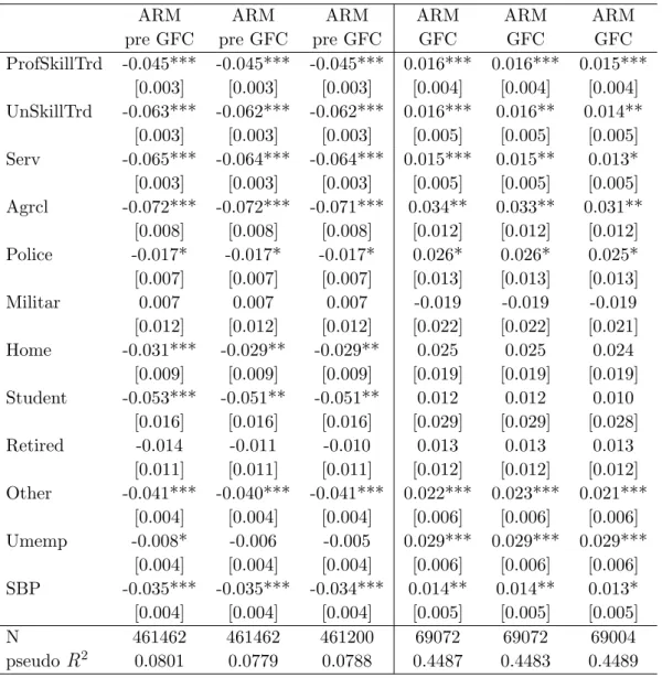
The interest in this paper focuses on the significant changes in the marginal effects of explanatory variables, particularly borrower characteristics, between the pre-GFC sample and the period affected by the crisis (that is pre and post September 2008). Table 6 sum-marizes the changes between the pre-GFC period and the GFC period in the estimates. These are collected by the change in effect; where marginal effects changed from signifi-cantly negative to signifisignifi-cantly positive or vice versa, from significant to insignificant or from insignificant to significant.

The first 11 categories identified relate to employment status. Public-sector employees are likely to be over-represented in the categories of employment status listed in Table 6. These applicants may have had relatively low income in the pre-crisis period. In each case, during the pre-GFC period an applicant in these employment categories had a significantly lower probability of taking an ARM than the benchmark 40 year old professional male, reflecting the higher income risk they generally faced. In the higher-risk GFC period, however, applicants in these employment categories had income relativities which were not much changed, but their jobs were relatively more secure than before. In the GFC sample, therefore, they were significantly more likely to select an ARM than the 40 year old professional male.

The second category of changes between the two periods reflects characteristics that significantly reduced the probability of choosing an ARM in the pre-GFC sample, but now have no impact on that choice. These include large loans, young applicants, female applicants, with young dependants, and some employment categories. Compared with the benchmark 40 year old male applicant with no dependants, these applicants have borrower characteristics consistent with desiring a loan with less income risk. In the pre-crisis period they could obtain this result, however, in the crisis period, these characteristics are

(17)

not recognized in their outcomes. They are not able to obtain a loan which is significantly differentiated from that offered to the benchmark 40 year old single male. It appears that these categories of applicant took on more risk than before, which would indicate inefficiency. However, these cases deserve further investigation which will be explored in future work. For example, if banks responded to higher risk by offering these applicants ARMs on more stringent terms than average (a lower loan-to-value ratio, for instance), they would be less likely to choose ARMs than in the pre-crisis period.

In the pre-crisis period, applicants with limited time at their current address had a higher probability of choosing an ARM, but that is no longer evident in the crisis period where the effect is insignificant. Older borrowers, with significant time with the bank and a more significant financial literacy as represented by the number of credit facilities they possess, are also no longer able to express their previous higher preference for an ARM as they did the pre-GFC period – these characteristics make no difference compared with the benchmark applicant in the GFC period.

While mixed, the results suggest that the bank has reduced its risk by offering terms under which applicants find it difficult to express different choices in terms of income and mobility risk. Rather, these characteristics are now dominated by the purely finan-cial characteristics of the market and the application. In a number of cases related to occupational category, the bank has acted to return risk to the applicant.

In addition the bank seems to use some previously unused borrower characteristics to further reduce its risk. In the pre-GFC period results the marital status of the applicant or the presence of a co-borrower had no impact on the probability of choosing an ARM. In the GFC period, however, these characteristics are now some of the few which reduce the probability of choosing an ARM over the benchmark single applicant. This represents a reduction in repayment risk to the bank.

The changing nature of the financial environment clearly affects both parties to the mortgage agreement. In the GFC period, the cash rate exerts a negative influence on the probability of an ARM product, whereas it previously had no marginal effect. In addition, higher bank fees and higher gross monthly income and house price inflation decrease the probability of an ARM loan in the crisis period, whereas these characteristics and conditions tended to increase the probability of an ARM loan prior to the crisis. This likely reflects a reduction in the expected potential capital gains and lower leverage desired during the aftermath of the major reduction in wealth experienced by almost all home owners (via the Australian compulsory superannuation scheme as a minimum exposure). In these conditions banks may well be able to charge higher fees for the wealth and income risk reducing CM products.

(18)

provide mixed evidence as to the way in which product choices change. In the pre-crisis period borrowers had been able to access products which were generally aligned with preferences to reduce income, mobility and wealth risk as revealed by their borrower characteristics. Although mortgage cost variables, particularly interest rate differentials, dominate the probability of selecting a CM in preference to an ARM, there is plentiful evidence that borrower characteristics play a statistically significant role in modifying their choices.

During the crisis period, however, some of these formerly significant effects are al-tered in a way which suggests that these risks are being transferred to the borrower. In some instances, it appears that the terms on which mortgages are offered change so that relatively low-risk applicants choose an ARM. In other cases, the borrower is bearing the income risk in the crisis period. Mobility risk is also being transferred back to the borrower, who no longer have an increased probability of an ARM loan. Finally, the loan decision now uses other previously unutilised information on income risk in the household, via the presence of another adult member (married or co-borrower).

The richness of the dataset and the fortuitous occurrence of the global financial crisis during the sample period have allowed this paper to demonstrate for the first time that borrower characteristics do contain information which is used in the mortgage decision making process. As conditions change the borrower characteristics are unchanged, but their influence on the mortgage product application outcome changes significantly. The directions of these changes are consistent with the bank seeking to reduce its risk during a period of increased cost of funds by changing the terms of the contract or seeking to retain more of the risk of individual mortgages with the applicants.

6 Conclusion

The range of mortgage products available to households is not infinite. Products are segmented and the market is incomplete. As a consequence we would expect to find that borrower characteristics are a significant determinant of mortgage product choice, but the existing empirical literature has not consistently found this result. There are several possible reasons for this outcome. Data quality is one possibility – many datasets do not contain borrower characteristics or these characteristics are imputed from other sources. Another possibility relates to institutional structures - the majority of studies relate to the US where GSEs provide a semi government guarantee to the securitization of standard housing loans, allowing mortgage issuing financial institutions to quickly and easily divest themselves of a substantial amount of risk.

(19)

re-flects risk sharing between the household borrower and the financial institution using data from the Australian market. In this market households choose between ARM prod-ucts and complex mortgage (CM) prodprod-ucts such as honeymoon discounts or periodically renegotiated fixed rate contracts. FRMs as commonly investigated for the US do not exist. Consistent with existing empirical literature, we find that mortgage cost variables such as the interest rate differential between the products, and the prevailing economic conditions such as house price inflation and unemployment rate, influence the probability of borrowers selecting a mortgage product in the anticipated manner.

Using our detailed dataset on mortgage applications we find that borrowers facing income risk and wealth risk are more likely to choose products which reduce their initial repayments, that is CM products, while those facing mobility risk are more likely to choose flexible products, such as an ARM. The results are in concordance with those anticipated in the literature, but rarely empirically confirmed.

Further, the occurrence of the global financial crisis during our sample period provides a natural experiment as to how the influence of these characteristics changes when the bank faces an increased cost of holding risky assets on its balance sheet. Estimations from the crisis period show that in contrast to the pre-crisis period, borrowers are now less able to reduce their income and mobility risk; these aspects either do not influence the probability of choosing a CM product over an ARM, or move to act in the opposite direction. In addition, the mortgage application outcome shows evidence that the bank now takes into account borrower characteristics on income risk which were previously ignored in order to minimize its holding of risk. The results from the pre-crisis and crisis period samples on mortgage applications convincingly illustrate the use of information on income, wealth and mobility risk in risk sharing between the mortgage applicant and the bank under different market conditions.

(20)

References

[1] Amromin, G. and Huang, J. and Sialm, C. and Zhong, E.(2011), ‘Complex mort-gages’, National Bureau of Economic Research

[2] ANZ (2008), ANZ Survey of adult financial literacy in Australia: Final Report, available at http://www.anz.com/Documents

/AU/Aboutanz/AN 5654 Adult Fin Lit Report 08 Web report full.pdf

[3] Australian Prudential Regulation Authority (2008), ‘ADI housing lending’, APRA Insight, Issue 1, 18-24.

[4] Bateman, H., Eckert, C., Geweke, J., Louviere, J.J., Thorp, S., Satchell, S. (2012), ‘Financial competence and expectations formation: Evidence from Australia’, The Economic Record, 88, 39-63.

[5] Berndt, A. and Hollifield, B. and Sand˚as, P. (2010), ‘The role of mortgage brokers in the subprime crisis’, National Bureau of Economic Research

[6] Brown, A., Davies, M., Fabbro, D., and Hanrick, T. (2010), ‘Recent developments in banks’ funding costs and lending rates’, Reserve Bank of Australia Bulletin, March, 35-44.

[7] Brueckner, J.K.(1994), ‘Borrower mobility, adverse selection, and mortgage points’,

Journal of Financial Intermediation, 3, 416-441.

[8] Brueckner, J.K. and Follain, J.R.(1988), ‘The rise and fall of the ARM: An econo-metric analysis of mortgage choice’,The Review of Economics and Statistics, 93-102. [9] Campbell, J.Y.(2006), ‘Household Finance’, The Journal of Finance, 61, 1553-1604. [10] Campbell, J.Y. and Calvet, L.E. and Sodini, P.(2009), ‘Measuring the financial

so-phistication of households’, The American Economic Review, 118, 393-398

[11] Campbell, J.Y. and Cocco, J.F.(2003), ‘Household risk management and optimal mortgage choice’, The Quarterly Journal of Economics, 99, 1449-1494.

[12] Coulibaly, B. and Li, G.(2009), ‘Choice of mortgage contracts: Evidence from the survey of consumer finances’, Real Estate Economics, 37, 659-673.

[13] Davies, M.(2009), ‘Household debt: implications for monetary policy and financial stability’, Bank for International Settlements BIS Paper No.46, May, 19-30.

(21)

[14] Debelle, G.(2008), ‘A Comparison of the US and Australian housing markets’, Re-serve Bank of Australia Bulletin, June, 35-46.

[15] Debelle, G.(2009), ‘Whither Securitisation?’, Australian Securitisation Conference, Sydney, 18 November

[16] Debelle, G.(2010), ‘The state of the mortgage market’, Address to Mortgage Inno-vation Conference, Sydney, Reserve Bank of Australia, 30 March

[17] Dhillon, U.S. and Shilling, J.D. and Sirmans, C.F.(1987), ‘Choosing between fixed and adjustable rate mortgages: note’, Journal of Money, Credit and Banking, 19, 260-267.

[18] Dungey, M. and Wells, G. and Thompson, S.(2011), ‘First home buyers support schemes in Australia’, Australian Economic Review, 44, 468-479.

[19] Ellis, L.(2006), ‘Housing and housing finance: the view from Australia and beyond’,

Reserve Bank of Australia Research Discussion Paper

[20] Fortowsky, E. and LaCour-Little, M. and Rosenblatt, E. and Yao, V.(2011), ‘Housing tenure and mortgage choice’, The Journal of Real Estate Finance and Economics, 42, 162-180.

[21] La Cava, G. and Simon, J.(2005), ‘Household debt and financial constraints in Aus-tralia’, Australian Economic Review, 38, 40-60.

[22] Leece, D.(2000), ‘Household choice of fixed versus floating rate debt: a binomial probit model with correction for classification error’, Oxford Bulletin of Economics and Statistics, 62, 61-82.

[23] Lusardi, A. and Mitchell, O.(2007), ‘Financial literacy and retirement preparedness: evidence and implications for financial education’, Business Economics, 42, 35-42. [24] Miles, D.(2004), ‘The UK mortgage market: Taking a longer-term view’, Final

Re-port and Recommendations

[25] Miles, D.(2005), ‘Incentives information and efficiency in the UK mortgage market*’,

The Economic Journal, 115, 82-98.

[26] Ortalo-Magne, F. and Rady, S.(2006), ‘Housing market dynamics: On the contribu-tion of income shocks and credit constraints’, The Review of Economic Studies, 73, 459-485.

(22)

[27] Paiella, M. and Pozzolo, A.F.(2007), ‘Choosing between fixed and adjustable rate mortgages’,University of Molise, Dept. SEGeS, Economics and Statistics Discussion Papers

[28] Sa-Aadu, J. and Sirmans, C.F.(1995), ‘Differentiated contracts, heterogeneous bor-rowers, and the mortgage choice decision’, Journal of Money, Credit and Banking, 27, 498-510.

(23)

Table 1: ARM characteristics for loans from banks, October 20107

Features Common- ANZ Bendigo Westpac Bank of

wealth Queensland Rate 7.36% 7.41% 7.45% 7.51% 7.51% Comparison Rate 7.49% 7.52% 7.59% 7.64% 7.63% Establishment Fee $600 $600 $230 $600 $495 Service Fee $8 $5 $8 $8 $10 LVR 80% 80% 80% 80% 80% LMI 97% 95% 97% 95% 95%

Early Repayment Yes Yes Yes Yes Yes

Redraw Yes* Yes Yes* Yes Yes

Interest Only Yes Yes# _No _Yes# _Yes#

Offset Account Yes Yes No Yes Yes*

Table 2: FRM characteristics for loans from banks, October 20108

Features Common-wealth ANZ Bendigo Westpac Bank of Queensland

Fixed period 1-15 1-10 1-5 1-10 1-5 Rate 5y 7.79% 7.74% 7.99% 7.89% 7.84% Comparison Rate 7.69% 7.65% 8.14% – 7.78% Establishment Fee $600 $600 $230 $600 $495 Service Fee $8 $10# _$8 _$8 _$10 LVR 80% 80% 80% 80% 80% LMI 97% 95% 97% 95% 95%

Early Repayment Yes” _Yes” _Yes” _Yes” _Yes”

Redraw No No Yes∗ Yes∗ No

Interest Only Yes Yes# No Yes# Yes

Offset Account Partial Partial No No Yes∗#

7_Notes: ∗_{includes a fee,} #_{for a limited period}

Rate refers to the interest rate current for the first fortnight of October 2010. Comparison Rate is calculated and published by each bank on the basis of secured credit of $A150,000 over a 25 year termbased on monthly repayments. Establishment Fee is an upfront fee which could be a combination of application fee and an establishment or settlement fee. Service Fee is a monthly fee (this is in prices for the first fortnight of October, 2010). LVR refers to the maximum Loan-to-Value Ratio accepted by the bank. LMI refers to the LVR offered if Loan Mortgage Insurance (LMI) is contracted. Early repayment refers to the possibility of early payments to reduce the outstanding principal balance and the term of the loan. Redraw offers to withdraw additional payments already made. Interest Only gives the option to reduce the monthly commitments by paying only the interest amount due each month. Offset Account is an add-on that links an existing personal account from the bank with the home loan where the borrower is able to offset the funds in the account against the loan. All prices are October 2010; at that time the target cash rate was 4.50 percent.

8_Notes: ∗_{includes a fee,} #_{for a limited period} ”_{for a limited amount}

Fixed period considers the fixed periods in years offered by each bank. Rate 5y only shows the fixed interest rate calculated for a 5 year fixed loan. The rest of the rows have the same definition as the Standard ARM table. All prices are of October 2010; at that time the Reserve’s Bank target cash rate was 4.50 percent.

(24)

Table 2a: EM characteristics for loans from banks, October 2010

Features CommonWealth ANZ Bendigo Westpac Bank of Queensland

Rate 8.46% 7.56% 7.55% 7.66% 7.86% Comparison Rate 8.55% 7.65% – 7.64% – Establishment Fee $950 $600 $230 $600 $495 Service Fee $12 $12.5 $8 $10 $10 LVR 65-86%” _– _80% _80% _80% LMI – 97% 90% 95% 90%

Early Repayment – No No Yes Yes

Redraw Yes Yes No Yes∗ –

Interest Only Yes Yes – Yes Yes

Offset Account – No – No –

Rollover No – – – –

Table 2b: HM characteristics for loans from banks, October 2010

Features Common- ANZ Bendigo Westpac Bank of

wealth Queensland

Discount period 12 months - - - 12 months

Rate 6.66% 6.71% 6.95% 6.81% 6.51% Comparison Rate 7.41% 6.76% 7.01% 6.86% 7.52% Establishment Fee $600 $600 $230 $600 $495 Service Fee $8 $0 $0 $0 $10 LVR 80% 80% 80% 80% 80% LMI 95% 95% 97% 95% 95%

Early Retirement Yes Yes Yes Yes Yes

Redraw Yes* Yes Yes* Yes* Yes

Interest Only Yes Yes# - Yes# Yes#

(25)

Table 3: Summary Statistics by Mortgage Type Mar 2003 - Aug 2008: Mortgage Cost variables: Medians (Standard Deviations): all values are in 1989-1990 $A.

Variable CM ARM Total

Loan Amount $104399 $130697 $117264 (64535) (99026) (87703) Term (years) 30 30 30 (15.07) (6.68) (11.23) Repayment (monthly) $680 $883 $781 (487) (796) (697) Mortgage Payment $684 $895 $790 (471) (750) (661)

Mortgage interest rate 6.95% 7.07% 7.07%

(0.94) (0.77) (0.85)

Bank fee $410 $422 $416

(105) (106) (107)

Ratio of bank fee to 0.40% 0.35% 0.38%

mortgage fee (0.53) (0.93) (0.79)

Payment to income ratio 7.70% 7.70% 7.70%

(15.27) (15.83) (15.60)

Debt service ratio 42.64% 44.59% 43.69%

(15.78) (18.30) (17.32)

Loan-to-value ratio 65.64% 64.40% 64.94%

(20.04) (21.72) (21.07)

Loan to income ratio 2.50 2.50 2.50

(1.54) (2.31) (2.02)

Value of property $190539 $220723 $207246

(111833) (666186) (515286)

(26)

Table 4: Summary Statistics by Mortgage Type Mar 2003 - Aug 2008: Borrower Characteristics variables: Medians (Standard Deviations)

Variable CM ARM Total

Age 39 40 39 (10.57) (10.54) (10.56) No of Dependents 0 0 0 (1.12) (1.09) (1.10) Age Youngest Dpndnt 5 5 5 (4.89) (5.04) (4.99)

Years current address 4 4 4

(6.50) (6.82) (6.70)

Years prev address 0 0 0

(4.58) (4.33) (4.43)

Years current employ 4 4 4

(6.79) (7.00) (6.92)

Years prev employ 0 0 0

(3.26) (3.38) (3.33)

Gross Monthly Income $3650 $4368 $4078

(2678) (3104) (2969)

Net Monthly Income $2962 $3446 $3253

(1699) (1945) (1869)

H’hold Gross Income $3688 $4438 $4139

(2798) (3204) (3077)

NonDurables Exp $812 $837 $828

(406) (398) (402)

Liquid Assets $10513 $14438 $12817

(46673) (52800) (50648)

Short term Liabilities $708 $797 $761

(10074) (7926) (8817)

Credit Score 514 544 533

(189) (182) (185)

(27)

Table 5: Fitted ARM Interest Rates

RAT EARM RAT EARM RAT EARM RAT EARM

pre-GFC GFC pre-GFC GFC

Fitted Fitted Fitted SB Fitted SB

IntrbnkRt 0.031 5.845*** 0.184*** 5.865*** [0.033] [0.113] [0.031] [0.113] SVarHRate 1.079*** 0.000 1.466*** 0.000 [0.015] [0.000] [0.014] [0.000] CDSwap5yAA -0.124*** -0.822*** -0.435*** -0.828*** [0.008] [0.038] [0.008] [0.038] OIS1m -0.507*** -1.547*** -1.117*** -1.555*** [0.020] [0.055] [0.019] [0.055] TerDRav 0.155*** -0.630*** 0.284*** -0.634*** [0.011] [0.066] [0.010] [0.066] TerDRavsp 0.034*** 1.107*** 0.020*** 1.116*** [0.005] [0.038] [0.005] [0.038] SAccDR 0.006 -15.653*** -0.013*** -15.703*** [0.004] [0.417] [0.004] [0.417] CAccDR 0.032*** 9.142*** 0.041*** 9.170*** [0.002] [0.260] [0.002] [0.260] YldCrv -0.035*** -0.673*** -0.064*** -0.673*** [0.003] [0.023] [0.003] [0.023] SBpreA 0.472*** [0.003] SBgfcA -0.122*** [0.015] cons 0.773*** 7.787*** -0.155*** 7.802*** [0.028] [0.199] [0.028] [0.198]

Regional D Yes Yes Yes Yes

N 270428 56233 270428 56233

R2 _0.8328 _0.7827 _0.8507 _0.7830

Standard errors in brackets

(28)

Table 6: Fitted CM Interest Rates

RAT ECM RAT ECM RAT ECM RAT ECM

pre-GFC GFC pre-GFC GFC

Fitted Fitted Fitted SB Fitted SB

SFxdHRate 0.219*** 1.871*** 0.223*** 1.865*** [0.007] [0.128] [0.007] [0.123] SVarHRate 0.879*** 0.000 0.843*** 0.000 [0.013] [0.000] [0.013] [0.000] CDSwap5yAA -0.178*** 1.022*** -0.155*** 1.039*** [0.008] [0.071] [0.008] [0.069] OIS1m 0.160*** -2.191*** 0.198*** -2.178*** [0.015] [0.221] [0.015] [0.212] TerDRav -0.100*** -2.424*** -0.112*** -2.450*** [0.016] [0.177] [0.016] [0.172] TerDRavsp -0.038*** 0.874*** -0.037*** 0.888*** [0.008] [0.110] [0.008] [0.106] SAccDR -0.076*** 13.886*** -0.074*** 13.856*** [0.007] [0.738] [0.007] [0.718] CAccDR -0.020*** -10.179*** -0.021*** -10.148*** [0.002] [0.547] [0.002] [0.534] YldCrv -0.019*** -0.603*** -0.018*** -0.605*** [0.005] [0.073] [0.005] [0.070] SBpreC 0.042*** [0.003] SBgfcC 0.189*** [0.012] cons -1.229*** -6.159*** -1.212*** -6.316*** [0.045] [0.640] [0.045] [0.617]

Regional D Yes Yes Yes Yes

N 191034 12839 191023 12824

R2 _0.8494 _0.6789 _0.8495 _0.6904

Standard errors in brackets

(29)

Table 7: APE Probit Regressions Pooled: pre GRC Mar 2003 - Aug 2008; GFC Sep 2008 - Dec 2009

ARM ARM ARM ARM ARM ARM

pre GFC pre GFC pre GFC GFC GFC GFC

Mortgage Cost RfDiff -0.472*** 0.328*** [0.015] [0.086] RATEDIFFap -0.064*** -0.094*** [0.003] [0.012] RATEDIFFapsb -0.061*** -0.105*** [0.003] [0.013] BnkFeeF 0.490*** 0.501*** 0.505*** -0.146*** -0.143*** -0.128*** [0.008] [0.008] [0.008] [0.012] [0.012] [0.012] RpymntF 0.247*** 0.248*** 0.264*** 0.395*** 0.396*** 0.407*** [0.003] [0.003] [0.003] [0.011] [0.011] [0.012] LoanAg500 -0.056** -0.051* -0.053* 0.091 0.089 0.088 [0.021] [0.021] [0.021] [0.097] [0.096] [0.097] LVR -0.003*** -0.003*** -0.003*** -0.001*** -0.001*** -0.001*** [0.000] [0.000] [0.000] [0.000] [0.000] [0.000] DSR -0.003*** -0.003*** -0.003*** -0.006*** -0.006*** -0.006*** [0.000] [0.000] [0.000] [0.000] [0.000] [0.000] Market conditions IntrbnkRt -0.006 -0.019*** [0.004] [0.003] YldCrv 0.011*** 0.005 [0.003] [0.006] InfAll -0.005* -0.005* -0.005* -0.114*** -0.031** -0.030** [0.002] [0.002] [0.002] [0.029] [0.011] [0.011] InfH 0.013*** 0.017*** 0.016*** 0.114*** -0.027*** -0.034*** [0.002] [0.002] [0.002] [0.024] [0.008] [0.009] UnmplymntRt -0.081*** -0.009*** -0.010*** -0.045** 0.108*** 0.114*** [0.004] [0.002] [0.002] [0.015] [0.011] [0.011] ExpctdInfln 0.010*** 0.015*** 0.015*** -0.013* 0.054*** 0.062*** [0.002] [0.001] [0.001] [0.006] [0.012] [0.013]

Standard errors in brackets *ρ¡0.05, **ρ¡0.01, ***ρ¡0.001

(30)

Table 7 continued: APE Probit Regressions Pooled: pre GRC Mar 2003 -Aug 2008; GFC Sep 2008 - Dec 2009

Borrower Characteristics Age30 -0.021*** -0.022*** -0.022*** 0.007 0.006 0.006 [0.002] [0.002] [0.002] [0.004] [0.004] [0.004] Age50 0.014*** 0.014*** 0.014*** -0.002 -0.002 -0.002 [0.002] [0.002] [0.002] [0.004] [0.004] [0.004] Age60 0.043*** 0.042*** 0.042*** -0.004 -0.004 -0.003 [0.003] [0.004] [0.004] [0.006] [0.006] [0.006] Age60plus 0.073*** 0.072*** 0.072*** -0.014 -0.013 -0.012 [0.005] [0.005] [0.005] [0.008] [0.008] [0.008] Female -0.020*** -0.020*** -0.020*** 0.005 0.005 0.004 [0.002] [0.002] [0.002] [0.003] [0.003] [0.003] Married 0.003 0.003 0.003 -0.007* -0.007* -0.007* [0.002] [0.002] [0.002] [0.003] [0.003] [0.003] AgeDpndntU5D -0.020*** -0.021*** -0.021*** -0.000 -0.000 -0.001 [0.002] [0.002] [0.002] [0.003] [0.003] [0.003] CoBorrwr -0.002 -0.002 -0.004 -0.020*** -0.021*** -0.021*** [0.002] [0.002] [0.002] [0.003] [0.003] [0.003] FTB 0.026*** 0.028*** 0.028*** 0.025*** 0.027*** 0.027*** [0.003] [0.003] [0.003] [0.006] [0.006] [0.006] SelfEmpl -0.005* -0.005* -0.005* -0.020*** -0.020*** -0.020*** [0.002] [0.002] [0.002] [0.003] [0.003] [0.003] tcuraddrssl2 0.004* 0.004* 0.004* -0.003 -0.003 -0.003 [0.002] [0.002] [0.002] [0.003] [0.003] [0.003] tcuraddrssg5 -0.033*** -0.033*** -0.034*** -0.013*** -0.013*** -0.014*** [0.002] [0.002] [0.002] [0.002] [0.002] [0.002] GrssMnthlyIncm 0.016*** 0.010*** 0.009*** -0.013*** -0.013*** -0.013*** [0.002] [0.002] [0.002] [0.003] [0.003] [0.003] PTIR 0.003*** 0.003*** 0.004*** 0.005*** 0.005*** 0.005*** [0.000] [0.000] [0.000] [0.000] [0.000] [0.000]

(31)

xyageincm -0.000*** -0.000*** -0.000*** 0.000 0.000 0.000 [0.000] [0.000] [0.000] [0.000] [0.000] [0.000] xyrtdincm -0.027*** -0.061*** -0.061*** 0.001 0.001 0.001 [0.002] [0.002] [0.002] [0.004] [0.004] [0.004] SrplsG 0.000*** 0.000*** 0.000*** -0.000*** -0.000*** -0.000*** [0.000] [0.000] [0.000] [0.000] [0.000] [0.000] LAssts -0.000*** -0.000*** -0.000*** -0.000 -0.000 -0.000 [0.000] [0.000] [0.000] [0.000] [0.000] [0.000] STLiab -0.001*** -0.001*** -0.001*** -0.001*** -0.001*** -0.001*** [0.000] [0.000] [0.000] [0.000] [0.000] [0.000] NonDExp -0.004* -0.006** -0.007** -0.019*** -0.020*** -0.020*** [0.002] [0.002] [0.002] [0.004] [0.004] [0.004] twithBnk 0.004*** 0.004*** 0.004*** 0.000** 0.000** 0.001*** [0.000] [0.000] [0.000] [0.000] [0.000] [0.000] NCrAccts -0.048*** -0.030*** -0.031*** [0.001] [0.001] [0.001] NcrFclty 0.011*** 0.011*** 0.011*** -0.004* -0.004 -0.003 [0.001] [0.001] [0.001] [0.002] [0.002] [0.002] Shares 0.008* 0.011** 0.011** [0.003] [0.003] [0.003] Occupation Dummies SemiProf -0.033*** -0.032*** -0.033*** 0.014* 0.013* 0.012* [0.004] [0.004] [0.004] [0.006] [0.006] [0.006] Mngm -0.019*** -0.019*** -0.019*** 0.001 0.001 0.001 [0.003] [0.003] [0.003] [0.004] [0.004] [0.004] Tech 0.003 0.003 0.003 0.009 0.009 0.009 [0.004] [0.004] [0.004] [0.007] [0.007] [0.007] Office -0.031*** -0.031*** -0.030*** 0.009 0.010 0.009 [0.003] [0.003] [0.003] [0.005] [0.005] [0.005] Sales -0.054*** -0.054*** -0.054*** 0.016** 0.015** 0.014* [0.003] [0.003] [0.003] [0.006] [0.006] [0.005]

(32)

ProfSkillTrd -0.045*** -0.045*** -0.045*** 0.016*** 0.016*** 0.015*** [0.003] [0.003] [0.003] [0.004] [0.004] [0.004] UnSkillTrd -0.063*** -0.062*** -0.062*** 0.016*** 0.016** 0.014** [0.003] [0.003] [0.003] [0.005] [0.005] [0.005] Serv -0.065*** -0.064*** -0.064*** 0.015*** 0.015** 0.013* [0.003] [0.003] [0.003] [0.005] [0.005] [0.005] Agrcl -0.072*** -0.072*** -0.071*** 0.034** 0.033** 0.031** [0.008] [0.008] [0.008] [0.012] [0.012] [0.012] Police -0.017* -0.017* -0.017* 0.026* 0.026* 0.025* [0.007] [0.007] [0.007] [0.013] [0.013] [0.013] Militar 0.007 0.007 0.007 -0.019 -0.019 -0.019 [0.012] [0.012] [0.012] [0.022] [0.022] [0.021] Home -0.031*** -0.029** -0.029** 0.025 0.025 0.024 [0.009] [0.009] [0.009] [0.019] [0.019] [0.019] Student -0.053*** -0.051** -0.051** 0.012 0.012 0.010 [0.016] [0.016] [0.016] [0.029] [0.029] [0.028] Retired -0.014 -0.011 -0.010 0.013 0.013 0.013 [0.011] [0.011] [0.011] [0.012] [0.012] [0.012] Other -0.041*** -0.040*** -0.041*** 0.022*** 0.023*** 0.021*** [0.004] [0.004] [0.004] [0.006] [0.006] [0.006] Umemp -0.008* -0.006 -0.005 0.029*** 0.029*** 0.029*** [0.004] [0.004] [0.004] [0.006] [0.006] [0.006] SBP -0.035*** -0.035*** -0.034*** 0.014** 0.014** 0.013* [0.004] [0.004] [0.004] [0.005] [0.005] [0.005] N 461462 461462 461200 69072 69072 69004 pseudo R2 _0.0801 _0.0779 _0.0788 _0.4487 _0.4483 _0.4489

(33)

Table 8: Changes in the P(ARM=1) between the pre-GFC period (Mar 2003 - Aug 2008) and the GFC period (Sep 2008 - Dec 2009). The symbols denote statistically significant positive (+) and negative (-) and insignificant (0) marginal effects on the probability of choosing and ARM loan.

Characteristics Pre-GFC GFC

Unemployment Rate - +

Semi-Professional (Prof.) - +

Sales (Prof.) - +

Professional Skilled Trade (Prof.) - +

Unskilled Trade (Prof.) - +

Service (Prof.) - +

Agriculture (Prof.) - +

Police (Prof.) - +

Other (Prof.) - +

Small Business Proprietor (Prof.) - +

Unemployed (Prof.) 0 +