Working Paper 09-29 Departamento de Economía de la Empresa Business Economics Series 03 Universidad Carlos III de Madrid
March, 2009 Calle Madrid, 126
28903 Getafe (Spain)
Fax (34-91) 6249607
THE VALUE OF A “FREE” CUSTOMER
Sunil Gupta, Carl F. Mela, and Jose M. Vidal-Sanz
∗Abstract
Central to a firm's growth is the profit potential of its customer base. However, customer lifetime value research is silent about customer profitability in networked setting wherein two populations of buyers and sellers interact (e.g., auction sites, job agencies). Often buyers pay no fees to the firm making them difficult to value. Yet buyers generate value by attracting fee-paying sellers. We present a model to value these "free" customers wherein buyer and seller growth arise from marketing actions and direct and indirect network effects. The firm chooses pricing and
advertising to maximize its long run profits subject to growth constraints. By relaxing these constraints by one customer, we impute the resulting lifetime customer value implications for the firm. We apply our model to auction data. Our results show strong direct and indirect network effects in our data. We find that in the most recent period the marginal buyer is worth more than the marginal seller. We also find our approach substantially better estimates of firm value than models that fail to consider network effects.
Keywords: Customer Lifetime Value; CRM; Dynamic Programming, GMM Estimation.
∗
Sunil Gupta (sgupta@hbs.edu) is the Edward W. Carter Professor of Business Administration, Harvard Business School, Soldiers Field, Boston, Massachusetts 02163. Carl F. Mela (mela@duke.edu) is a Professor of Marketing, The Fuqua School of Business, Duke University, Durham, North Carolina, 27708. José M. Vidal-Sanz (jvidal@emp.uc3m.es) is an Associate Professor of Econometric Theory and Marketing, Universidad Carlos III de Madrid, Calle Madrid 126, 28903 Getafe, Spain. We thank seminar participants at the Bilkent University, Emory University, University of Florida, Marketing Dynamics Conference, Marketing Science Conference, and Yale Center for Customer Insights Conference for their comments. Thanks are due to Mercedes Esteban-Bravo for her support checking the numerical codes.
1
Introduction
Metrics of customer value are becoming more important as firms are increasingly compelled to justify the role of marketing investments on firm profitability. A central metric for assessing the profitability of customers is customer lifetime value (CLV); the present value of all future profits generated by a customer (Kamakura et al. 2005). Using CLV afirm can rank order its customers or classify them into tiers based on their expected profitability. This allowsfirms to appropriately allocate resources across high versus low value customers (Reinartz and Kumar 2003, Rust, Lemon and Zeithaml 2004, Venkatesan and Kumar 2004). CLV can also be used for making customer acquisition decisions such that a firm does not spend more on acquiring a customer than the CLV of that customer (Gupta and Lehmann 2003, Gupta and Zeithaml 2006). It allowsfirms to balance their resources between customer acquisition and customer retention (Reinartz, Thomas and Kumar 2005). Recent studies also show that CLV can provide a link between customer value andfirm value (Gupta, Lehmann and Stuart 2004, Gupta and Lehmann 2005, Kim, Lim and Lusch 2008, Kumar and Shah 2009).
Current models of CLV, however, omit an important element. Consider the case of Monster.com, an employment market place where job-seekers post their resumes andfirms sign up tofind potential employees. Monster provides this service free to job-seekers and obtains revenue by charging fees to the employers. A natural question arising from this business model is how much Monster should spend to acquire a seeker. Traditional models of CLV can not answer this question since job-seekers do not provide any direct revenue. In fact, if one includes the cost of maintaining resumes, the standard CLV for a job-seeker is negative. However, without job-seekers employers will not sign up, and without the employers Monster will have no revenues or profits. In other words, the value of job-seekers is through their indirect network effect on job listers. This indirect network effect is not limited to employment services only (e.g., Monster, Hotjobs, Craiglist) but also extends to any exchange with multiple buyers and sellers (e.g., eBay, real estate).
The purpose of this study is to assess customer value when two parallel populations (e.g., buyers and sellers) interact and have strong direct (within population) and indirect (across populations) network effects. In these situations typically one set of customers (e.g., sellers) provide direct
financial returns to the company. For example, sellers provide commissions to real estate agencies. However,firms must acquire and maintain the other set of customers (e.g., buyers). These customers are "free" as they do not provide any direct revenue. Our objective is to develop a model to assess the value of both types of customers.1 This enables us to answer the following questions:
• How large are direct and indirect network effects? Large network effects suggest the potential for firms with strong network effects to dominate markets as the network grows. We find sizable indirect network effects in our data, especially for the buyer on the seller.
• How much should a company spend to acquire new customers in the presence of these network effects? For example, how much should Monster spend on acquiring an additional job-seeker, how much should PayPal spend on acquiring a new account, how much should a dating service spend for a new client, how much should an auction house spend to acquire a new buyer? In our context, wefind the value of a buyer to be quite substantial even though they provide no direct revenue to thefirm.
• How does the value of a customer change over time? Because the magnitude of network effects is likely to be time-dependent, customer value should also change over time. This suggests that the maximum amount of money that afirm should spend on a“free” customer changes over the life of a company. Our results suggest that customer value increases with the network size.
• How do we apportion value between buyers and sellers? In other words, how much of the value arising from the exchange between buyers and sellers accrues from each set of customers? Currently, firms have no metrics to apportion these revenues or profits. Our discussions withfirms indicate that some apportion all value to sellers since they generate the revenues. However, this clearly understates the value of buyers. Others use an arbitrary rule of thumb (e.g., 50-50) to split the profits between buyers and sellers. However, this implicitly assumes that both parties are equally important, which may not be necessarily correct. We find the value of buyers to exceed that of sellers.
• How should firms’ marketing efforts change over time in the presence of network effects? Marketing actions may be more critical in the early stages and network effects may dominate in later stages of a firm’s life cycle. Hence, there is an indirect link between customer acquisition and marketing spend, and this should logically affect customer valuation. Wefind customers to be most sensitive to marketing early in the life of thefirm.
• Does the omission of network effects understate the value of the customer base and hence the value of a firm? Our estimate of firm valuation is almost one-third of the observed market capitalization of thefirm in thefinal year of our data, and three-fourth of the market value observed in March 2009. In contrast, analogous approaches that ignore network and marketing effects yield an estimate of 2.5% of market capitalization.
Our research makes contributions to two research streams — customer valuation and diffusion modeling. With regard to the former, we are not aware of any study that examines customer value in the presence of indirect network effects. When ignored, the implied customer lifetime value of free customers (e.g., buyers) is zero. Such an implication runs counter to investments frequently made byfirms to attract these free users. Some research has explicitly considered the role of direct network effects within populations on customer lifetime value. Hogan, Lemon and Libai (2004) estimate the value of a lost customer by accounting for the word-of-mouth or direct network effects andfind these effects to be very large. Kumar, Petersen and Leone (2007) asses customers’referral value and find that while 68-81% of the customers intended to refer the service to their friends, only 30-33% actually did, and less than 15% of these referrals generated customers. Indirect effects between populations have also been shown to be substantial (e.g., Aregentisi and Filistrucci (2006), Gupta, Jain and Sawhney (1999), Katz and Shapiro (1985, 1986), Neil, Kende and Rob (2000), Rochet and Tirole (2006), Ryan and Tucker (2007), Wilbur (2008), Yao and Mela (2008)). Given these effects can be sizable, and that the implication of ignoring them is that free customers are worthless it seems sensible to address this limitation to the customer lifetime value literature.
With regard to the diffusion modeling literature, to the best of our knowledge this is the first empirical paper that endogenizes marketing spend by explicitly considering the firm resource al-location problem. In contrast, most empirical diffusion literature has addressed endogeneity via instrumental variables (Desiraju, Nair and Chintagunta 2004; Kim, Lee and Kim 2005). Yet an
explicit accounting of thefirm problem yields at least two tangible benefits. First, it is problematic to estimate diffusion models with a limited number of periods (Van den Bulte and Lilien 1997). By integrating the supply side information with a flexible Generalized Method of Moments (GMM) estimator, we exploit additional information thereby obtaining more reliable model estimates. Sec-ond, as we shall show, a proper accounting of thefirm’s decisions is necessary to impute customer value. Stronger network effects, for example, can enablefirms to raise prices thereby having positive consequences for customer value. Of course, the cost of solving the supply side model is increased complexity of analysis and estimation.
The paper proceeds as follows. We begin by developing a model that captures the growth of buyers and sellers from three sources — marketing actions (price and advertising), direct network effects or word-of-mouth, and indirect network effects. Next we define the firm’s problem as an optimal control problem wherein the firm chooses its marketing actions to maximize its long run profits subject to the growth of these populations. These growth constraints imply costates or Lagrangian multipliers for the optimization problem yielding the incremental profits to afirm arising from an additional buyer or seller; that is, the lifetime value of that incremental seller or buyer to the firm. We apply our model to data obtained from an auction house, and estimate the model using GMM based on both the growth and the Euler equations. This estimation approach explicitly exploits the endogeneity of marketing actions to increase the efficiency of the model estimates. We use the resulting parameter estimates to address the managerial questions highlighted above. We then conclude with limitations and next steps.
2
A Model of Customer Value in the Presence of Network E
ff
ects
Our model description follows in three stages. We begin by outlining the consumer demand system. Next, we discuss the supply side model. We conclude by outlining our estimation approach. Our application pertains to an anonymous auction house that operates largely as a monopoly market though the model can be generalized to other contexts.
2.1
Customer Growth and Network E
ff
ects
Consider two parallel populations of buyers and sellers interacting via a common platform in a monopoly context.2 The acquisition of customers in each group can be captured by a "diff
usion-2It is possible to extend this demand model to a duopoly context by adding additional growth equations and
cross-firm network effects. In our context we refrain from doing so because thefirm in our application is largely a monopoly. We leave the inclusion of competition in our model as an avenue for future research.
type" model as follows:3 NtB+1−NtB = µ a(At) +b NtB MB +g NtS MS ¶¡ MB−NtB¢+et, (1) NtS+1−NtS = µ α(pt, At) +β NS t MS +γ NB t MB ¶¡ MS−NtS¢+εt (2)
where NtB and NtS are the number of buyers and sellers at time t,MB and MS are the potential market size of buyers and sellers, a and α are functions of the platform marketing strategy and
(et, εt)are errors that capture omitted factors.
Some of the key characteristics of this system of equations are as follows:
1. The function a(At) recognizes that a firm can accelerate the growth of its buyers through buyer-targeted marketing. In our application of the e-auction house this takes the form of television and Internet advertising. Consistent with prior literature (e.g., Horsky and Simon 1983), we further assume that a(At) = a0 +φlnAt where At denotes advertising. In other words, there are diminishing marginal returns from advertising and the coefficient φ determines buyers’ responsiveness to firm’s advertising. The term a0 captures "organic" growth. If the term is negative, there is a tendency for persons to attrite from the system. In our application, advertising is the main vehicle for acquiring customers, but in other applications other marketing variables could be included.
2. Similarly, the termα(pt, At)highlights the fact that the growth of sellers depends on the mar-keting strategy used by the platform to attract sellers. In our context, price (defined as average commission percentage) is the key decision variable and it can change over time. Advertising can also influence the growth of sellers. We assume that α(pt, At) = α0−θlnpt+∆lnAt. Here the parameters θ and ∆ indicate sellers’ sensitivity to firm’s pricing and advertising respectively and α0 indicates “organic” seller growth. As in the buyer model, additional marketing covariates could be incorporated.4
3. The direct network effect for buyers and sellers is captured by the second term in equations (1) and (2). Hogan, Lemon and Libai (2003) used a similar term to capture the direct network effect of losing a customer. The parameters b and β effectively capture three effects. First, they account for word-of-mouth effect. As more people join the auction site, it may have a positive impact on other people. Second, as indicated earlier, they implicitly account for
3Similar models have also been used in the context of international diffusion of products (Kumar and Krishnan
2002). There are two alternative views to see how customer defection is implictly captured in this model. First, this model is similar to the repeat purchase model of Lilien, Rao and Kalish (1981), but augmented with marketing and indirect network effects. Second, one can explicitly model defection by adding a term for it in each equation. However, if the number of customers who defect a firm is proportional to the number of current customers, it is generally not possible to identify the defection parameters separately from the direct network effect (which is also proportional to the number of current customers). Some studies get around this problem by specifying the defection rate exogenously (Gupta et al. 2004, Libai, Muller and Peres 2008). However, this is rather ad-hoc and we prefer to model it implictly as per the above equations.
4Thefirm in our application also uses personal selling to attract sellers. However, this accounts for less than10%
defection. If defection is proportional to the number of current customers, then it will have a negative impact of parametersb and β. Finally, these parameters also capture the crowding effects where, all else equal, a buyer (or seller) prefers less competition (Roson 2005). This would imply a negative direct effect of an additional buyer or seller. The net result across these various behaviors may be a positive or negative parameter of direct effects.
4. As afirm acquires more buyers it becomes more attractive for sellers to join the firm as well. The reverse is also true— the more sellers a firm has, the more buyers it is likely to attract. This indirect network effect is captured by the third term in equations (1 and 2). The value of the parametersg and γ indicate the strength of indirect network effects.
5. The(et, εt)are errors that are assumed to follow a Markov process.5 These errors can reflect omitted factors.
2.2
Optimal Marketing Policies and Customer Value
Equations (1) and (2) characterize the growth of buyers and sellers as a result of firm’s actions (advertising and pricing), as well as direct and indirect network effects. The objective of the monopolisticfirm is to choose its advertising and pricing policies in such a fashion that it maximizes its long run profits.6 Specifically, thefirm solves the following discrete time problem:7
max {pt,At} E0 "∞ X t=0 (1 +i)−t¡NtSSpt−At ¢# s.t. NtB+1 = NtB+ µ a0+φlnAt+b NtB MB +g NtS MS ¶¡ MB−NtB¢+et (3) NtS+1 = NtS+ µ α0−θlnpt+∆lnAt+β NtS MS +γ NtB MB ¶¡ MS−NtS¢+εt
5The Markovian assumption can be relaxed (e.g., we can consider a VAR(p) process expressed in the space of
states). In our estimation, the residuals follow a seasonal VAR(1) model, i.e. errors from the same month of last year are correlated.
6In the case of a duopoly, an analogous profit function for a competingfirm leads to a Nash game in prices and
advertising. Moreover, the constraints expand to include cross-firm indirect and direct effects.
7These are "as if" models. In other words, we do not expect managers at thisfirm to be actually solving complex
dynamic models. Instead, via trial and error managers discover the decision rule that yields the highest profits (Little 1996). We tested our model with the a model which does not impose any optimality constraints. The assumption of optimality were not rejected by the data in our empirical application.
subject to initial values N0S = 0, N0B = 0 wherep is the average percent commission and S is the average revenue per seller.8 In compact notation, thefirm problem can be expressed as
max {pt,At} E0 "∞ X t=0 δtG¡NtB, NtS, pt, At¢ # NtB+1 = gB¡At, NtB, NtS, et ¢ (4) NtS+1 = gS¡pt, At, NtB, NtS, εt ¢
where δ= (1 +i)−1. The solution satisfies the first-order conditions associated with the following Lagrangian function, L¡©pt, At, NtB, NtS, λBt , λSt ª¢ = E0 "∞ X t=0 δtG¡NtB, NtS, pt, At ¢# + ∞ X t=0 λBt+1¡NtB+1−gB¡At, NtB, NtS, et ¢¢ + ∞ X t=0 λSt+1¡NtS+1−gS¡pt, At, NtB, NtS, εt ¢¢ . (5)
We would like to highlight a few characteristics of equations (3)-(5). First, the profits for thefirm depend directly on the number of sellers and the price thefirm charges them. If there is no indirect network effect of buyers on sellers, the number of buyers is irrelevant for profit maximization. In such a situation a firm has no reason to spend any money on buyer-oriented advertising and it has no way of assessing the long-term value of a buyer. This highlights the importance of indirect network effects in our context.
Second, CLV and customer equity assess customer profitability over the long-run. In a sim-ilar fashion, our formulation explicitly accounts for long run profitability of current and future customers.
Third, the lagrangian multipliers λBt and λSt in equation (5) provide a natural metric for the CLV of buyers and sellers at timet. These parameters represent the constraints on profits arising from not being able to add one customer at timet. As such, in the optimal solution,λBt provides the customer value of an incremental buyer acquired at time t over an infinite horizon, i.e. the effect of an additional buyer on the long-term discounted profit of the company. Thus, estimates of the buyer and seller CLV are outputs of our model. Analogously, λSt provides the customer value of an additional seller acquired at time t.
Fourth, the value of an additional buyer or seller varies over time. This intuitively makes sense as the network effects vary over the lifecycle of the company. For example, in the early stages of
8Average revenue per seller S increases over time (slightly above inflation), as do the number of buyers and sellers.
To test for potential endogeneity we regress S on buyer and seller growth andfind no significant correlation (p<0.60 for sellers and p<0.12 for buyers). The marginal costs in our application are close to zero and therefore we exclude them from our analysis.
a company, marketing actions may be more important to attract customers, while in the growth phase direct and indirect network effects may dominate. In other words, our model allows us to
find out the maximum amount of money afirm should spend to acquire a "free" buyer at different points in time.
Finally, unlike traditional CLV models, our model suggests that a firm’s actions (price and advertising) can influence customer growth and hence the overall value of thefirm. In other words, price and advertising decisions are dynamic and endogenous. As a result, they are affected by customer acquisitions and should therefore be considered when computing CLV. An incremental customer, by strengthening network effects, can lead to a reduced need for marketing spend and hence higher CLV. As we discuss next, endogenous marketing spend has additional implications for model estimation.
2.3
Model Estimation
2.3.1 Historical ApproachesIn many cases the purpose of diffusion model estimation was simply to assess the impact of a marketing variable on the diffusion process (Kamakura and Balasubramanian 1988, Jain and Rao 1990). For example, Simon and Sebastian (1987) investigate the impact of advertising on the diffusion of new telephones in West Germany. These studies are descriptive in nature and do not attempt to provide optimal advertising or pricing policies to maximizefirm’s profits.
In other cases, researchers have combined these models with analytical models of profit maxi-mization and optimal marketing policies of the firm in two distinct stages. In the first stage these studies ignore the optimal control problem of the firm and use the actual prices and advertising of the firm as exogenous variables when estimating the growth model of demand. In the second stage, they “plug-in” the parameter estimates of price and advertising in the optimal solutions of advertising and price to arrive at the optimal path for these decision variables and compare the optimal and actual values (e.g., Horsky and Simon 1983, Kalish 1985, Chintagunta and Vilcassim 1992, Chintagunta and Rao 1996). This stream of empirical research has two key limitations in our application. First, deterministic dynamic models are not necessarily close to the conditional mean of the true data generation process, and typical recursive forecast cannot be applied due to the nonlinearity of diffusion models and Jensen’s inequality. Second, standard time-discretization of continuous time models can generate biases in the parameter estimates of a stochastic continu-ous time model. Stochastic discrete time processes are a convenient approach, but in this context ignoring the supply dynamic optimization conditions in estimation can lead to inefficient estimates. A parallel group of studies explore the dynamic policies in a purely theoretical fashion using the solutions of the optimal control problem and examining the comparative statics or using numerical illustrations (e.g., Feichtinger, Hartl and Sethi 1994, Thompson and Teng 1984, Horsky and Mate 1988, Dockner and Jorgensen 1988). These theoretical approaches provide directional results but are not very useful if the objective is to provide empirical estimates in a particular application.
2.3.2 Our Estimation Approach
We consider a GMM based procedure that treats firm’s actions (price and advertising) as endoge-nous and at the same time considersfirm’s objective function of maximizing long run profits. This implies two points of departure from prior literature. The first point of difference is that we use
GMM for parameter estimation, obviating the need to specify conditional probability distributions for the model errors (as required by maximum likelihood), making the approach quite general and rendering asymptotically optimal estimates across a broad range of potential distributions. The second point of difference is that we consider the firm problem, increasing the efficiency of our estimates via exploiting additional information (as the supply side generates additional moment conditions).
To obtain our estimation equations, we define the optimal value function of the firm for an arbitrary initial point ¡NS
0, N0B, e0, ε0 ¢ as: V ¡N0S, N0B, e0, ε0 ¢ = max {pt,At} E0 "∞ X t=0 δtG¡NtB, NtS, pt, At ¢# . (6)
Then, the Jacobi-Bellman condition states that the solution satisfies for each integert≥0, V ¡NtB, NtS, et, εt ¢ = max pt,At © G¡NtB, NtS, pt, At ¢ +δEt £ V ¡NtS+1, NtB+1, et+1, εt+1 ¢¤ª . (7)
From the Jacobi-Bellman dynamic programing condition we obtain the following Euler equations (for details on the derivation see Appendix A1) ,
Et ⎡ ⎢ ⎣ µ NS tS −θ(MS−NS t)/pt −1 φ(MB−NB t )/At −Ht ¶ +δ ⎛ ⎜ ⎝ µ 0 Spt+1 ¶ −Dt+1 µ NtS+1S (−θ(MS−NS t+1)/pt+1) −1 φ(MB−NB t+1)/At+1 − Ht+1 ¶⎞ ⎟ ⎠ ⎤ ⎥ ⎦= 0, (8)
whereD and H are defined in Appendix A1. The system of conditional moments in equation (8), one for price and the other for advertising, can be denoted by
Et
£
U¡Ω0, NtB, NtS, pt, At, NtB+1, NtS+1, pt+1, At+1
¢¤
= 0, (9)
whereΩ0 denotes the true parameter vector. The Law of Iterated Expectations (see, e.g., Shirvaev 1991) implies that, for any instrumentZt predetermined at timet,the unconditional expectations are zero, i.e.,
E£U¡Ω0, NtB, NtS, pt, At, NtB+1, NtS+1, pt+1, At+1
¢
Zt
¤
= 0, (10)
In addition we have the two moment conditions associated with the dynamics of the state variables (the growth of buyers and sellers), yielding:
E ∙µ NtB+1−NtB− µ a0+φlnAt+b NtS MS +g NtB MB ¶¡ MB−NtB¢ ¶ Zt ¸ = 0, (11) E ∙µ NtS+1−NtS− µ α0−θlnpt+∆lnAt+β NtB MB +γ NtS MS ¶¡ MS−NtS¢ ¶ Zt ¸ = 0, (12)
where Zt are the instruments described in Section (2.3.3). It is these four equations (price and advertising paths, buyer and seller growth models) crossed with each instrument that form the basis of our estimation equations.
Note, if we ignore thefirm’s optimization problem and simply estimate the diffusion models, we get equations (1) and (2) corresponding to the buyers and sellers. This is the typical approach of empirical studies in the past as indicted in section 2.3.1. However, by explicitly incorporating the optimal control problem of thefirm we have additional equations as given by (10). These additional equations provide structure to the problem, leading to more efficient estimates and helping to identify the model parameters in the empirical estimation. Details on the GMM estimation are provided in Appendix A2).
2.3.3 Discount Rate and Instruments
We assumefirm’s monthly discount rate i= 0.015. This monthly discount rate of 1.5% translates into an approximate annual discount rate of 20%. Given the limited number of variables, we use two lags for the instruments. The use of lags for instruments is common and as we shall show, these appear to be good instruments (e.g., Kadiyali, Chintagunta, and Vilcassim 2000).9 Specifically,Zt is a9×1 vector
Zt=
¡
1, NtS−1, NtS−2, NtB−1, NtB−2,logpt−1,logpt−2,logAt−1,logAt−2
¢0
(13) and since we have 4 equations, we use 36 moment equations and 10 parameters (with 26 degrees of freedom). These instruments are tested via Hansen’s (1982) test of overidentifying restrictions, orJ-statistic (see Appendix A2).
3
Application
The application of our model requires information on the number of sellers and buyers over time as well as the marketing expenditures invested in the acquisition of these customers. An anonymous auction house provided monthly data on these quantities for its largest market between February 2001 and December 2006. Thefirm obtains revenues from sellers who list items on its web site for auction. These revenues are obtained from a listing fee, some promotional fees and a commission on the sales proceeds. These are combined into an overall margin value by thefirm and this is the measure used in our application. If S is the average annual gross merchandise sold per seller, and pt is the percentage commission charged by the auction house at timet, thenfirm’s annual margin from each seller isSpt. The marginal cost in this business are close to zero and therefore we exclude them from our analysis. The buyers provide no direct revenue to the firm. Not surprisingly the
firm has a greater interest in acquiring and maintaining its sellers even though it recognizes that it needs to have buyers for its auctions. While sellers push thefirm to acquire more buyers, the firm is not sure of how to value these buyers— which is the central question of our research.
The auction house spends money on TV and Internet advertising to attract buyers. The TV advertising data were compiled quarterly which we converted to monthly data by dividing by three
9
As indicated earlier, the residuals in our application follow a seasonal VAR(1) model, i.e. errors from the same month of last year are correlated. Further, wefind almost no correlation between errors at other times.
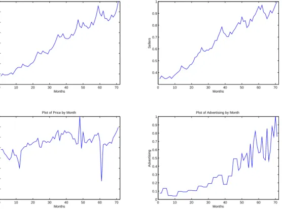
to create a monthly series.10 In addition, the firm provided information on margins and total transacted volume. To protect the confidentiality of the firm, we are unable to report the specific data means, but in Figure 1 we present information regarding the number of customers and the marketing expenditures over time, normalized so that the maximum value of each series is one.
0 10 20 30 40 50 60 70 0.2 0.3 0.4 0.5 0.6 0.7 0.8 0.9 1 B u y e rs Months Plot of Buyers by Month
0 10 20 30 40 50 60 70 0.4 0.5 0.6 0.7 0.8 0.9 1 S e lle rs Months Plot of Sellers by Month
0 10 20 30 40 50 60 70 0.6 0.65 0.7 0.75 0.8 0.85 0.9 0.95 1 P ri c e ( R e la ti v e B le n d e d M a rg in ) Months Plot of Price by Month
0 10 20 30 40 50 60 70 0 0.1 0.2 0.3 0.4 0.5 0.6 0.7 0.8 0.9 1 A d v e rt is in g Months Plot of Advertising by Month
Figure 1: Changes in Marketing and Demand Over Time
The upper left and right panels of Figure 1 indicate rapid growth in the number of buyers and sellers. There are approximately 4.6 buyers for each seller. The pricing data depicted in the lower left panel indicates that percent commission is increasing slightly over time, a sign of increasing pricing power which may arise from the growth of the buyer-seller network. This trend suggests it is desirable to account for pricing power and the endogeneity of pricing when computing the value of a customer. Advertising also shows an increase over time which may be due tofirm’s increasing concern of attracting new buyers over time or it may be due to reduced advertising sensitivity in the market prompting the firm to spend more to achieve the same results as before.
We have 71 monthly observations in our data. We break these observations into two components for the empirical analysis; a calibration dataset (comprised of thefirst 65 months) and a validation
1 0
Because we have monthly advertising spend for 18 of the months and all Internet advertising spend is monthly, the correlation between the smoothed and non-smoothed series is 0.96. Hence there is little practical consequence of this transformation.
data set (comprised of the last 6 months).11 It is worth noting that the forecasts of future sales and marketing require solving the Bellman recursions in equations (6) and (7)—a non-trivial challenge in as much as the procedure is analytically and computationally demanding. We discuss this forecasting procedure in Section 4.5.
4
Results
4.1
Model Fit
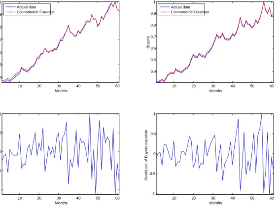
The overall model fit is given by the statistic J = T ·QcW³Ωb´, where QWc³Ωb´ is defined in Appendix A2. The J statistics is distributed χ2r−k where r is the number of equations andk the number of parameters. For our empirical applicationJ = 9.89,r= 36and k= 10.Therefore with P rob[χ2(26) > J] = 0.9982 we accept the overidentifying moment conditions. In other words, the moment conditions are close to zero and the instruments are orthogonal to the error. In Figure 2 we present the model fit and the estimation residuals.
For diagnosis purposes, we considered three alternatives or models. Thefirst approach ignores the supply side equations and therefore treats marketing actions as exogenous. This is similar to the traditional diffusion modeling. GMM estimation of this model reveals two things. First, a Likelihood Ratio type test show that we can not reject the hypothesis that our supply side constraints are binding (χ2(11) = 3.48, p >0.1). Second, all parameters of this null model (except the market size estimates) are insignificant. This illustrates that the supply side constraints put structure on the model that help identify parameters (Chintagunta et al. 2006). We also performed a simulation showing that the estimation errors are reduced when the conditions (10) are included. The second alternative model assumes thatfirms are myopic in pricing and advertising decisions. We estimate this model by assuming a very high discount rate. Estimating this model without the supply side constraints provides similar results to the ones for thefirst model described above. This is not surprising since the discount rate is used only for computing CLV, and does not enter the parameter estimates without the supply constraints. When supply constraints are added to this model, it did not converge. This suggests that the observed price and advertising data that enter the supply side are inconsistent with the myopic view.
The third model tests the sensitivity of market size estimates by forcing them to double the values estimated by our model and re-estimating other parameters. We find that this null model performs significantly worse than our model. Compared to our model, the standard error of the residuals from this model are 5.5 times larger for the buyers and 8.7 times larger for the sellers.
4.2
Parameter Estimates
Table 1 presents the parameter estimates of our model along with the t-statistics.
1 1
Prior research shows that it is generally difficult to estimate market size of diffusion models unless the data series show an inflection point. Figure 1 shows that thefirm in our application is still in growth phase. Two factors help us identify market size paramaters. First, we have a large number of data points compared to typical diffusion study. As Van den Bulte and Lilien (1997) show this helps estimate market size parameters better. Second, we use the supply side equations to put structure on our model which also help identify these parameters (Chintagunta et al. 2006).
10 20 30 40 50 60 0.4 0.5 0.6 0.7 0.8 0.9 1 Months S e lle rs Actual data Econometric Forecast 10 20 30 40 50 60 0.4 0.5 0.6 0.7 0.8 0.9 1 Months B u y e rs Actual data Econometric Forecast 10 20 30 40 50 60 -1 -0.5 0 0.5 1 R e s id u a ls o f S e lle rs e q u a ti o n Months 10 20 30 40 50 60 -1 -0.5 0 0.5 1 R e s id u a ls o f B u y e rs e q u a ti o n Months
Figure 2: Model Fit and Residuals
Parameter Estimate t-stat Buyers Equation
Intercept a0 0.002 5.56
Advertising ($) φ 0.0001 50.71
Direct Network Effect of Buyers b −0.016 −5.82
Indirect Network Effect of Sellers g 0.003 3.93
Potential Market Size of Buyers (million) MB 47.07 51.65 Sellers Equation
Intercept α0 −0.003 −1.41
Price (%) θ 0.005 4.78
Advertising ($) ∆ 0.0014 2.99
Direct Network Effect of Sellers β −0.177 −7.00
Indirect Network Effect of Buyers γ 0.299 3.79
Potential Market Size of Sellers (million) MS 4.64 2.99 Table 1: Parameter Estimates
All parameters are statistically significant except the intercept in the seller growth equation. Advertising has a significantly positive impact on the acquisition of buyers and sellers. Price has a significant negative impact on sellers growth (recall α(pt, At) = α0−θlnpt+∆lnAt, so price parameterθis expected to be positive). The parametersbandβare negative.12 As discussed earlier, these parameters capture the net effect of word-of-mouth, customer defection and crowding. The negative sign suggests that customer defection is outpacing the growth from word-of-mouth effect. This may also be a result of "crowding" where customers prefer to list/buy when fewer competitors are in the system.
The indirect network effects for both buyers and sellers are positive and very strong. This suggests that the more buyers we have in the system the more sellers are attracted to the firm and vice versa. Further, the indirect effect of buyers on sellers (0.299) is significantly larger than the indirect effect of sellers on buyers (0.003). In other words, even though buyers do not provide any direct revenue to the firm, they may be more critical for its growth. We will return to this issue when we translate these into the value of buyers and sellers. In sum, in response to the first question we raised in the introduction of this paper, we find that there are significant network effects present in our empirical application.
The market potential for buyers is estimated to be about 47 million and the number of sellers is estimated to be about 4 million. Though we can not reveal the specifics regarding the current market size in order to protect the confidentiality of the firm, based on our market potential estimates the market penetration of both populations is on the order of 2/5 for sellers and 1/5 for buyers. This indicates that there are significant growth opportunities for thisfirm that should be reflected in its overall customer andfirm value.
4.3
The Value of a Customer
In this section, we address the three pertinent managerial questions we asked in the beginning of this paper.
1. What is the value of a buyer or a seller? In other words, what is the maximum the firm should spend on acquiring a buyer or a seller. This estimate is especially difficult for buyers who do not provide any direct revenue or profit to thefirm.
2. How can thefirm apportion the value of transactions between buyers and sellers? 3. How do these values change over time?
As indicated earlier, the value of a buyer is given by the Lagrangian multiplier of the optimal control problem. The shadow prices for buyers and sellers are given by (see Appendix (A3) for details): µ λBt λSt ¶ =δt ⎛ ⎜ ⎝ µ 0 Spt ¶ − µ D11 t Dt12 D21t Dt22 ¶ µ NS tS −θ(MS−NS t)/pt −1 φ(MB−NB t )/At −Ht ¶⎞ ⎟ ⎠. (14)
Using this equation and the model parameters we estimate the current value of a buyer as approximately $80 (at the request of the sponsoring firm, we have rescaled the data such that the
1 2
maximum buyer/seller value over the data period is $100). Note that the entire value of buyers is derived from their indirect network effect on the growth of sellers. Traditional models of CLV that do not account for these network effects are unable to estimate the value of these "free" customers. The estimated value of a seller at the current time is about $50. Surprisingly, on average, the value of a seller over time is significantly lower than that of a buyer; even though buyers outnumber sellers by 4.6 to 1. This is counter-intuitive for at least two reasons. Although the firm believes that buyers are important for its growth, its revenues are derived directly from sellers. Therefore, intuitively it makes sense to assume that the paying customers or sellers are more important for
firm’s profits. The second reason that supports the firm’s intuition is the fact that there are approximately 4.6 buyers for each seller. Since each transaction requires a buyer and a seller, it is reasonable to argue that the value of a seller should be at least 4.6 times the value of a buyer. Our model results go against this intuition and suggest that the value of a seller is less than half the value of a buyer.
What explains this counter-intuitive result? First, Table 1 indicates that the parameter value for the indirect network effect of buyers on sellers growth (0.299) is substantially larger than the parameter value for the indirect network effect of sellers on buyers growth (0.003). Second, the net effect of crowding and attrition on sellers is−0.177, suggesting a natural tendency to attrite. Third, prices have a negative impact on sellers’growth. Fourth, the negative intercept for seller’s equation (α0 =−0.003) suggests that there is no "organic" or "natural" growth of the seller population. In other words, except for the indirect network effect of buyers, all other factors are working against the growth of sellers. This makes the buyers even more critical for the overall growth and profitability of the firm. In the end, even though the firm has 4.6 buyers for each seller, the indirect network effect of a buyer is significantly greater than the indirect network effect of a seller. The net result of all these factors is such that the value of a buyer rivals that of the seller.
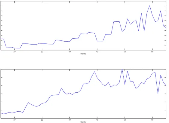
Does the buyer and seller value change over time? Figure 3 shows these values rescaled to 100 over the time frame of our data. As expected these values change significantly over time since the network effects vary over the lifecycle of the firm. Several important insights emerge from these results. First, the value of sellers is still growing while the value of buyers increased from time 0 to 40, but has been steady since. In the beginning, when thefirm has limited number or no customers, marketing actions are the primary source of driving traffic. As the number of customers grow, the network effects become more important. Because the growth of the firm in our application has not substantially slowed, it is not surprising to find that the network effects amplify over time. Eventually, the impact of network effects will diminish. As the firm reaches the market potential for its customers, the value of an additional buyer or seller will approach zero. In other words, the value of a buyer and a seller is likely to follow an inverted U-shaped curve.
4.4
Price and Advertising E
ff
ectiveness
Given the presence of strong network effects, how do the effectiveness of marketing actions change over time? To address this question, wefind the price and advertising elasticities, which are given by the following expressions.
10 20 30 40 50 60 0 10 20 30 40 50 60 70 80 90 100 L if e ti m e V a lu e o f M a rg in a l S e lle r Months 10 20 30 40 50 60 40 50 60 70 80 90 100 L if e ti m e V a lu e o f M a rg in a l B u y e r Months
Figure 3: Value of a Buyer and a Seller Over Time
⎛ ⎝ ∂gS(pt,At,NtB,NtS,εt) ∂pt pt NS t ∂gB(pt,At,NtB,NtS,εt) ∂pt pt NB t ∂gS(p t,At,NtB,NtS,εt) ∂At At NS t ∂gB(A t,NtB,NtS,et) ∂At At NB t ⎞ ⎠= µ −θNtS¡MS−NtS¢ 0 ∆NS t ¡ MS−NS t ¢ φNB t ¡ MB−NB t ¢ ¶ .
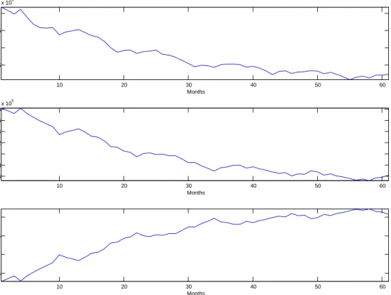
Figure (4) shows the trajectory of the advertising and price elasticity over time, for buyers and sellers respectively. Several interesting results emerge from thisfigure. First, both advertising and price elasticities are decreasing over time. In other words, as firms acquire more customers over time, network effects become increasingly important. This diminishes the impact of advertising and price on customer growth. Note that the decrease in advertising elasticities imply increased advertising spend is required to achieve the same level of advertising impact. Coupled with the increase in seller value over time, this impliesfirms would increase advertising over time, consistent with the observed data.
Second, both price and advertising elasticities are significantly smaller than the comparable numbers reported for consumer packaged goods. Specifically, wefind price elasticities in the range of−0.01to−0.03, in contrast to the average price elasticity of−1.6found by Tellis (1988) or−1.4
10 20 30 40 50 60 0.5 1 1.5 2 x 10⁻³ B u y e rs A d v . e la s ti c it y Months 10 20 30 40 50 60 0.6 0.8 1 1.2 1.4 1.6 1.8 x 10⁻³ S e lle rs A d v . e la s ti c it y Months 10 20 30 40 50 60 -0.025 -0.02 -0.015 -0.01 S e lle rs P ri c e e la s ti c it y Months
Figure 4: Advertising and Price Elasticity Over Time
found by Bijmolt et al. (2004). Similarly, our advertising elasticity estimates of a maximum of about
0.002 are significantly lower than the average ad elasticities of 0.05 for established products and
0.26for new products (Lodish et al. 1995). These differences are due to the nature of the business in our application, which is very different from the traditionally examined consumer packaged goods industry. In our application for an Internet auction, prices are commission rates which are relatively small component of the overall profits accruing to a seller (as these include the prices buyers pay). Further, the network externalities render price effects to be somewhat smaller. Using different data, Yao and Mela (2008)find auction house revenue-fee elasticities to be as low as -0.08. Advertising in our context is primarily through keywords on search engines. Recent studies show that click-through rates of these keywords are generally less than 1%. For example, Rutz and Bucklin (2007) find click-through rates in their study to be about 0.6%, which better reflect our ad elasticity estimates. With the changing landscape of advertising, the growth of new media and the explosion of viral marketing, the elasticities in our study may be more reflective of the current demand status in online businesses, especially in the presence of network effects.
4.5
Firm Value
4.5.1 Traditional Approaches
How do network effects influence the value of the customer base and hence the value of the firm? Hogan, Lemon and Libai (2003) incorporate direct network effects through a diffusion model to examine the value of a lost customer in online banking. They find that the CLV of a customer without direct network effects is about $208. However, direct network effects can be as large as $650 in the early stages of the diffusion process. Our work augments this research by considering the indirect network effects that are critical in a buyer-seller situation. In one setting wherein these effects might be considerable, Gupta et al. (2004) estimated the CLV at eBay. Using an annual discount rate of 20% and retention rate of 80%, Gupta et al. (2004) estimated the value of eBay to be 2.5% of its market capitalization in the period of their analysis. Commenting on the inability of their model to estimate the market value of eBay, they suggested, "...eBay is an auction exchange, and thus there may be significant network externalities that are not captured by the traditional diffusion model. Furthermore, eBay’s business includes both buyers and sellers ... it may be important to model buyers and sellers separately and then construct a model of interaction between them," (page 14). This is precisely what we have done in this paper.
4.5.2 A Dynamic Network Approach
We estimated firm value by considering the firm’s dynamic problem as outlined in equation (3). To achieve this objective we first need to forecast not only the growth in number of buyers and sellers as a result of direct and indirect network effects, but also the potential changes in optimal price and advertising levels that may influence the revenues and marketing expenses, and hence customer andfirm value. As a result, the computational demands of this task are exacerbated by the need to solve the stochastic dynamic programing problem in order to forecast future pricing and advertising levels. To address this problem, we develop a numerical method predicated upon the Euler equation, the available data and the implementation of Bootstrap techniques (see Appendix A4 for details). The result of this procedure is a set ofJ draws for the price, advertising and growth paths with a forecasting horizonL, that allow us to compute the probability distribution based on J realizations. Moreover, we use these simulates to compute the forecasted customer values (λt) for each simulated path and for each period of time T+ 1, ..., T+L.
Model Forecasts As future prices, advertising and sales are inputs into our calculation offirm value, we begin by assessing the forecasting accuracy of our model. As mentioned earlier, we retained six observations from the holdout period for this purpose. We use mean absolute percentage error (M AP E) as our measure of forecasting accuracy. Our results show that the M AP E for the number of buyers and sellers is 0.094 (or 9.4%) and 0.067(or 6.7%) respectively. These are good forecasts for any growth model. However, recall that we are not simply forecasting the number of buyers and sellers, which can be easily done using a standard diffusion model with direct and indirect network effects. Instead we need to forecast the optimal price and advertising expenditures of thefirm in the future. Network effects have a direct impact on these marketing instruments. We are not aware of any prior research that has done this type of forecasting.
Our forecast results show that theM AP Efor price is0.047(or4.7%) andM AP Efor advertising is0.426(or42.6%). In other words, while the forecasting accuracy for price is quite good, we are not
as accurate in predicting advertising expenditure. Note that this error is computed by comparing forecasted and actual advertising levels. Our sponsoringfirm may be setting its actual advertising levels using information (e.g., changes in advertising rates, migration of advertising spend into new channels, etc.) that are not explicitly included in our model and this may be reflected in the forecasts. Overall these are reasonable estimates given the complexity of forecasting the endogenous marketing variables as well as customer growth.
Firm Value Equipped with forecasts of demand, prices and advertising, one can forecast firm value by summing discounted profits over an infinite horizon. In particular, we note that the firm value at time T is given by:
V ( T, NT) = max {pt,At} E0 "∞ X t=T δt¡NtSSpt−At ¢# . (15)
To estimate this value, for each Bootstrap sample we consider the firm’s present value atT using
ρjT = L X t=T δt ³ NtjSSpjt −Ajt ´ . (16)
For a large forecasting horizon, L, the average for all the simulated realizations provides an esti-mation of thefirm value:
b V ( T, NT) = 1 J J X j=1 ρjT. (17)
We use a forecasting horizon of fifteen years (L= 12×15) and J = 3,000samples to estimate
firm market valueVb( T, NT) and compare it to thefirm’s actual market cap at the end of our data period. Thefirm in our application conducts significant business in international markets as well as in non-auction related businesses. Since our data in this paper only pertains to domestic auctions, we consider firm’s domestic auction revenues and profits while comparing our estimates of firm value to actual market value. Based on public sources we find domestic auctions to be about37%
of thefirm’s total global revenues at the end of 2006. Therefore, we use 37% of thefirm’s market cap as the benchmark against which we compare our estimates.
We find that our model accounts for about 1/3rd of the observed market cap. While this is significantly lower than the actual market cap, it compares favorably with Gupta et al. (2004) who could account for only2.5%of eBay’s market cap.
There are several possible reasons for ourfirm value estimate to be lower than the actual market value. First, our model may still be missing elements (e.g., option value) that need to be captured in future research. Second, we used37%allocation based on domestic market revenue for auctions in 2006. At that time, international markets and non-auction revenues were growing faster for our sponsoring firm, which is not reflected in this allocation. Finally, it is also possible that market was overvaluing this firm. As of March 2009, market cap of thisfirm (like most others) has come down significantly, and our estimates account for almost 3/4th of its current market cap.
5
Conclusions
Customer profitability is a central consideration to many firms. Though research in this area is burgeoning, little work to date addresses the issue of customer valuation in the context of direct and indirect network effects in a dynamic setting. This limitation is palpable because network effects exist in many contexts including sellers and buyers for auction houses, job seekers and job providers on job sites, real estate listings and buyers on listing services, and so forth. In such contexts, typically one set of customers (e.g., buyers in an auction or job-seekers on a job site) do not pay any direct revenue to thefirm. It is difficult to assess the CLV of these "free" customers using traditional CLV models. In addition, extant methods of valuing customers do not consider the role that customer acquisitions play in affecting marketing expenditures. This can also influence CLV, especially in the presence of network effects, asfirms can reduce their marketing expenses as a network grows and the reduction in costs further amplifies customer value.
We address these problems by offering a new approach to assess customer and firm value that is predicated upon the incremental profits to thefirm over an infinite horizon as a result of adding another buyer or seller to the firm’s portfolio of customers. To do this, we begin by developing a diffusion-type model of the growth in the firm’s buyer and seller populations over time. We then use this system of growth equations, coupled with margin data and marketing expenditures, to determine firm profits over time. Using the parameter estimates from this model, it is possible to compute the Lagrange multipliers arising from the constraints that the seller and buyer growth models place on a firms’infinite horizon profits. The Lagrange multiplier for buyers or sellers is a natural measure of the marginal impact of an additional buyer or seller on afirm’s net discounted sum of future profits, and hence provides the CLV of each type of customer.
Using data for an online auction house, we find strong evidence of network effects. Further, network effect of buyers on seller is significantly larger than the effect of seller on buyers. Our results show that each type of customer, including the "free" buyer, provides the firm with hundreds of dollars of value over the lifetime of the customer. Further, the value of a customer is increasing over time as the network builds. We also find that price and advertising elasticities reduce over time. As the network effects become stronger, marketing plays less of a role in attracting buyers and sellers thereby reducing the need to advertise. Our model provides an estimate of firm value that is significantly better than the ones provided by previous models.
Given the nascent state of customer valuation research in the context of network effects, there are many potential areas for future research. First, as richer data become available in more contexts, our analysis can be generalized. Second, our model can also be extended to multi-sided markets. For example, YouTube is a three-sided market with viewers, content providers and advertisers. Similarly, social networks are multi-sided markets where some users provide direct value to the
firm through their purchases while others provide indirect value through their influence on the network. Third, our analysis is developed in the context of a monopoly. While we believe this to be a reasonable characterization in our case because the auction house we consider is dominant in its market, there are many contexts where this is not the case. Fourth, our growth equations are predicated upon a diffusion framework. Though these provide a reasonable approximation to the optimal evolution of these states, richer structural characterizations might yield additional insights such as the role of customer heterogeneity in the growth of networks. Finally, we did not allow market potential of buyers and sellers to change over time. As Internet penetration increases, the potential market size may also change. In sum, we hope this initial foray into customer valuation
in the context of network effects leads to further research and additional insights that will be useful tofirms who are concerned with managing their customer portfolio in a networked economy.
References
[1] Bijmolt, Tammo H.A., Harald J. Van Heerde, and Rik G.M. Pieters(2004), "New
Empirical Generalizations on the Determinants of Price Elasticity,"Journal of Marketing Re-search, 42 (May), 141-156.
[2] Chamberlain, Gary S.(1987),"Asymptotic Efficiency in Estimation with Conditional Mo-ment Restrictions,"Journal of Econometrics, 34, 305-334.
[3] Chintagunta, Pradeep and Naufel Vilcassim (1992), "An Empirical Investigation of
Advertising Strategies in a Dynamic Duopoly," Management Science, 38 (9), 1230—1244.
[4] Chintagunta, Pradeep and Vithala Rao (1996), "Pricing Strategies in a Dynamic
Duopoly: A Differential Game Model," Management Science, 42 (11), 1501—1514.
[5] Chintagunta, Pradeep, Tulin Erdem, Peter Rossi and Michel Wedel (2006),
"Structural Modeling in Marketing: Review and Assessment," Marketing Science, 25 (6), 604-616.
[6] Desiraju, Ramarao, Harikesh Nair and Pradeep Chintagunta (2004), "Diffusion of
New Pharmaceutical Drugs in Developing and Developed Nations," International Journal of Research in Marketing, 21, 341-357.
[7] Dockner, Engelbert and Steffen Jorgensen (1988), "Optimal Pricing Strategies for
New Products in Dynamic Oligopolies,"Marketing Science, 7 (4), 315-334.
[8] Feichtinger, Gustav, Richard Hartl and Suresh Sethi (1994), "Dynamic Optimal
Control Models in Advertising: Recent Developments,"Management Science, 40 (2), 195-226.
[9] Gupta, Sachin, Dipak Jain and Mohanbir sawhney(1999), "Modeling the Evolution of
Markets with Indirect Network Externalities: An Application to Digital Television,"Marketing Science, 18 (3), 396-416.
[10] Gupta, Sunil and Donald R. Lehmann (2003), "Customers as Assets," Journal of Inter-active Marketing, 17, 1(Winter), 9-24.
[11] Gupta, Sunil and Donald R. Lehmann (2005), Managing Customers as Investments:
The Strategic Value of Customers in the Long Run, Wharton School Publishing, Upper Saddle River, New Jersey.
[12] Gupta, Sunil, Donald R. Lehmann and Jennifer Ames Stuart(2004), "Valuing
Cus-tomers,"Journal of Marketing Research, 41, 1, 7-18.
[13] Gupta, Sunil and Valarie Zeithaml (2006), "Customer Metrics and Their Impact on
Financial Performance,"Marketing Science, forthcoming.
[14] Hansen, Lars Peter(1982), "Large Sample Properties of Generalized Method of Moments Estimators,"Econometrica, 50, 4. (July), 1029-1054.
[15] Hogan, John, Katherine Lemon and Barak Libai(2003), "What is the True Value of a Lost Customer?"Journal of Service Research, 5, 3, February, 196-208.
[16] Horsky, Dan and Leonard S. Simon(1983), "Advertising and the Diffusion of New Prod-ucts,"Marketing Science, 2, 1(Winter), 1-17.
[17] Horsky, Dan and Karl Mate (1988), "Dynamic Advertising Strategies of Competing
Durable Good Producers,"Marketing Science, 7, 4(Fall), 356-367.
[18] Jain, Dipak C. and Ram C. Rao (1990), "Effect of Price on the Demand for Durables: Modeling, Estimation, and Findings," Journal of Business Economics and Statistics, 8(2), 163-170.
[19] Kadiyali, Vrinda, Pradeep Chintagunta, and Nafuel Vilcassim (2000),
"Manufacturer-Retailer Channel Interactions and Implications for Channel Power: An Em-pirical Investigation of Pricing in a Local Market,"Marketing Science, 19, 2 (Spring), 127-148. [20] Kalish, Shlomo(1985), "A New Product Adoption Model with Price, Advertising and
Un-certainty,"Management Science, 31, 12, 1569—1585.
[21] Kamakura, Wagner A, Carl F. Mela, Asim Ansari, Anand Bodapati, Pete Fader,
Raghuram Iyengar, Prasad Naik Scott Neslin, Baohong Sun, Peter Verhoef,
Michel Wedel, and Ron Wilcox (2005), "Choice Models and Customer Relationship
Management,"Marketing Letters, 16, 3/4, 279-291.
[22] Kamakura, Wagner A. and Siva Balasubramanian (1988), "Long-Term View of the
Diffusion of Durables: A Study of the Role of Price and Adoption Influence Processes via Tests of Nested Models,"International Journal of Research in Marketing, 5, 1-13.
[23] Katz, M. and C. Shapiro(1985), "Network Externalities, Competition, and Compatibility", American Economic Review, 75, 3, 424-440.
[24] Katz, M. and C. Shapiro(1986), "Technology Adoption in the Presence of Network Exter-nalities,"Journal of Political Economy, 94, 22-41.
[25] Kim, Oliver, Steve Lim and Robert Lusch (2008), "Marketing and Shareholdr Value:
Sales Capitalization and its Estimation,"MSI Working Paper Series, 08-003, 73-90.
[26] Kim, W., J. Lee and T. Kim(2005), "Demand Forecasting for Multigenerational Products Combining Discrete Choice and Dynamics of Diffusion Under Technological Trajectories," Technological Forecasting and Social Change, 72, 825-849.
[27] Kumar, V. and Trichy Krishnan(2002), "Multinational Diffusion Models: An Alternative Framework,"Marketing Science, 21, 3(Summer), 318-330.
[28] Kumar, V., J. Andrew Petersen, and Robert P. Leone(2007), "How Valuable is Word
of Mouth?"Harvard Business Review, 85, 10(October), 139—146.
[29] Kumar, V.and Dinsesh Shah (2009), "Expanding the Role of Marketing: From Customer
[30] Libai, Barak, Eitan Muller and Renana Peres(2008), "The Effect of Customer Attri-tion on Service Growth and Equity,"Journal of Marketing Research, forthcoming.
[31] Lilian, Gary, Ambar Rao and S. Kalish (1981), "Bayesian Estimation and Control of
a Detailing Effort in a Repeat Purchase Diffusion Enviornment,"Management Science, 27, 5, 493-506.
[32] Lodish, Leonard M., Magid Abraham, Stuart Kalmenson, Jeanne Livelsberger,
Beth Lubetkin, Bruce Richardson, and Mary Ellen Stevens (1995), "How T.V.
Advertising Works: A Meta-Analysis of 389 Real World Split Cable T.V. Advertising Experi-ments,"Journal of Marketing Research, 32, 2(May), 125—139.
[33] Neil, G., M. Kende and R. Rob (2000), "The Dynamics of Technological Adoption in
Hardware/Software Systems: The Case of Compact Disc Players," The RAND Journal of Economics, 31 (1), 43-61.
[34] Newey, Whitney K. and Daniel. McFadden (1994), "Large Sample Estimation and
Hypothesis Testing," in Handbook of Econometrics, vol. iv, ed. by R. F. Engle and D. L. McFadden, pp. 2111-2245, Amsterdam: Elsevier.
[35] Newey, Whitney K. and Kenneth D. West(1987), "A Simple, Positive Semi-Definite, Heteroskedasticity and Autocorrelation Consistent Covariance Matrix," Econometrica, 55, 3(May), 703-708.
[36] Reinartz, Werner and V. Kumar(2003), "The Impact of Customer Relationship
Char-acteristics on Profitable Lifetime Duration," Journal of Marketing, 67, 1(January), 77-99.
[37] Reinartz, Werner, Jacquelyn Thomas and V. Kumar(2005), "Balancing Acquisition
and Retention Resources to Maximize Customer Profitability," Journal of Marketing, 69, 1 (January), 63-79.
[38] Rochet, J.-C. and J. Tirole(2006). Two-sided Markets: A Progress Report,Rand Journal of Economics, forthcoming.
[39] Roson, Roberto(2005), "Two-Sided Markets: A Tentative Survey,"The Review of Network Economics, 4, 2 (June), 142 - 160.
[40] Rust, Roland, Katherine Lemon and Valarie Zeithaml(2004), "Return on Marketing:
Using Customer Equity to Focus Marketing Strategy,"Journal of Marketing, 68, 1(January), 109-126.
[41] Rutz, Oliver and Randolph E. Bucklin (2007), "A Model of Individual Keyword
Per-formance in Paid Search Ad,"Working Paper, Yale School of Management.
[42] Ryan, Stephen and Catherine Tucker(2007), "Heterogeneity and the Dynamics of Tech-nology Adoption," working paper, MIT.
[44] Simon, Hermann and Karl-Heinz Sebastian (1987), "Diffusion and Advertising: The German Telephone Campaign,"Management Science, 33, 4, 451-466.
[45] Tellis, Gerard. J. (1988), “The Price Elasticity of Selective Demand: A Meta-analysis of Econometric Models of Sales,”Journal of Marketing Research, 25, 331-341.
[46] Thompson, Gerald and Jinn-Tsair Teng(1984), "Optimal Pricing and Advertising Poli-cies for New Product Oligopoly Models,"Marketing Science, 3, 2(Spring), 148-168.
[47] Van den Bulte, Christophe and Gary Lilien(1997), "Bias and Systematic Change in the Parameter Estimates of Macro-Level Diffusion Models,"Marketing Science, 16 (4), 338-353.
[48] Venkatesan, Rajkumar and V. Kumar (2004),“A Customer Lifetime Value Framework
for Customer Selection and Resource Allocation Strategy,” Journal of Marketing, 68, 4(No-vember), 106-125.
[49] Viner, Jacob. (1931), “Cost Curves and Supply Curves,” Zeitschrift für Nationalökonomie, 3, 1, 23—46.
[50] Wilbur, Kenneth C.(2008), "A Two-Sided, Empirical Model of Television Advertising and Viewing Markets,"Marketing Science, 27, 3 (May-June), 356-378.
[51] Yao, Song and Carl F. Mela (2008), "Online Auction Demand," Marketing Science, 27, 5 (September), 861-885.
Appendix
A1
The Euler Equation
To solve the dynamic problem indicated by (3) we begin by defining the optimal value function: for an arbitrary initial point¡N0S, N0B, e0, ε0¢this function is given by:
V ¡N0S, N0B, e0, ε0¢= max {pt,At} E0 "∞ X t=0 δtG¡NtB, NtS, pt, At ¢# . (A-1)
Then, the Jacobi-Bellman condition states that the solution satisfies the following recursion for each period t≥0,13
V ¡NtB, NtS, et, εt¢= max pt,At ©
G¡NtB, NtS, pt, At¢+δEt£V ¡NtS+1, NtB+1, et+1, εt+1¢¤ª. (A-2)
Incorporating the state equations into (A-2) and settingV ¡NtB, NtS, et, εt
¢ ≡Vt;G ¡ NtB, NtS, pt, At ¢ ≡ Gt;gB ¡ At, NtB, NtS, et ¢ ≡gtB;and gS¡pt, At, NtB, NtS, εt ¢ ≡gtS leads to Vt= max pt,At{ Gt+δEt[Vt+1]}. (A-3)
Therefore, the first order conditions associated to the right hand side optimization problem are satisfied, which are (in matrix notation),
0 = µ∂Gt ∂pt ∂Gt ∂At ¶ +δ Ã ∂gS t ∂pt 0 ∂gS t ∂At ∂gB t ∂At ! × µEth∂Vt+1 ∂NS t+1 i Et h∂V t+1 ∂NB t+1 i ¶ 1 3Thoughp
tandAt appear ingB andgSin the right hand side of A-2, these variables are concentrated out of the
value function because the optimal levels ofpt and At depend only on the parameters inNB, NS, eand ε. Hence,
leading to µEth∂Vt+1 ∂NS t+1 i Et h ∂Vt+1 ∂NB t+1 i ¶ =−1 δ Ã ∂gS t ∂pt 0 ∂gS t ∂At ∂gB t ∂At !−1µ∂G t ∂pt ∂Gt ∂At ¶ = −1 δ ⎛ ⎜ ⎜ ⎝ 1 ∂gSt ∂pt 0 −∂gS1 t ∂pt ∂gSt ∂At ∂gB t ∂At 1 ∂gB t ∂At ⎞ ⎟ ⎟ ⎠ µ∂Gt ∂pt ∂Gt ∂At ¶ =−1 δ ⎛ ⎜ ⎜ ⎜ ⎜ ⎝ ∂Gt ∂pt ∂gSt ∂pt ∂Gt ∂At ∂gBt ∂At − ∂Gt ∂pt ∂gSt ∂pt ∂gSt ∂At ∂gBt ∂At ⎞ ⎟ ⎟ ⎟ ⎟ ⎠ (A-4)
where we have used that
µ A 0 B C ¶−1 = µ 1 A 0 −A1 B C 1 C ¶ .
Using the envelope theorem (Viner, 1931), it can be proved that
µ ∂Vt ∂NB t ∂Vt ∂NS t ¶ = µ∂Gt ∂NB t ∂Gt ∂NS t ¶ +δ ⎛ ⎝ ∂gB t ∂NB t ∂gS t ∂NB t ∂gBt ∂NS t ∂gtS ∂NS t ⎞ ⎠×Et ⎡ ⎢ ⎣ µ∂Vt+1 ∂NB t+1 ∂Vt+1 ∂NS t+1 ¶⎤ ⎥ ⎦. (A-5) Substituting Et h∂V t+1 ∂NB t+1 i andEt h∂V t+1 ∂NS t+1 i
from (A-4) into (A-5),
µ ∂Vt ∂NB t ∂Vt ∂NS t ¶ = µ∂Gt ∂NB t ∂Gt ∂NS t ¶ − ⎛ ⎝ ∂gB t ∂NB t ∂gS t ∂NB t ∂gB t ∂NS t ∂gS t ∂NS t ⎞ ⎠× ⎛ ⎜ ⎜ ⎜ ⎜ ⎝ ∂Gt ∂pt ∂gSt ∂pt ∂Gt ∂At ∂gB t ∂At − ∂Gt ∂pt ∂gS t ∂pt ∂gSt ∂At ∂gB t ∂At ⎞ ⎟ ⎟ ⎟ ⎟ ⎠ (A-6)
updating the resulting condition and combining it with the first order conditions (A-4) yields the system, 0 = µ ∂Gt/∂pt ∂gS t/∂pt ∂Gt/∂At ∂gB t/∂At − ∂Gt/∂pt ∂gS t/∂pt ∂gS t/∂At ∂gB t /∂At ¶ (A-7) +δ Et ⎡ ⎢ ⎢ ⎢ ⎢ ⎢ ⎣ µ∂Gt+1 ∂NB t+1 ∂Gt+1 ∂NS t+1 ¶ − ⎛ ⎝ ∂gB t+1 ∂NB t+1 ∂gS t+1 ∂NB t+1 ∂gB t+1 ∂NS t+1 ∂gS t+1 ∂NS t+1 ⎞ ⎠µ ∂Gt+1/∂pt+1 ∂gS t+1/∂pt+1 ∂Gt+1/∂At+1 ∂gB t+1/∂At+1 − ∂Gt+1 ∂pt+1 ∂gS t+1 ∂pt+1 ∂gS t+1 ∂At+1 ∂gB t+1 ∂At+1 ¶ ⎤ ⎥ ⎥ ⎥ ⎥ ⎥ ⎦
This expression is the Euler equations system. Note that the left hand side can be introduced in the conditional expectation with a sign change.
Computing the partial derivatives, we obtain the expression (8).
Et ⎡ ⎢ ⎣ µ NS tS −θ(MS−NS t)/pt −1 φ(MB−NB t )/At −Ht ¶ + (1 +i)−1 ⎛ ⎜ ⎝ µ 0 Spt+1 ¶ −Dt+1 µ NS t+1S (−θ(MS−NS t+1)/pt+1) −1 φ(MB−NB t+1)/At+1 −Ht+1 ¶⎞ ⎟ ⎠ ⎤ ⎥ ⎦= 0, (A-8) where Ht = ∂Gt/∂pt ∂ ∂ptg S t ∂ ∂Atg S t ∂ ∂Atg B t = N S t S −θ¡MS−NS t ¢ /pt · ∆¡MS−NtS¢ φ¡MB−NB t ¢= −N S t S∆pt θh¡MB−NB t ¢, (A-9) Dt+1 = µ D11 t+1 Dt12+1 Dt21+1 Dt22+1 ¶ with D11t+1 = 1 + µ b MB ¶¡ MB−NtB+1¢− à a0+φlnAt+1+b NB t+1 MB +g NS t+1 MS ! (A-10) = 1 +b−a0−φlnAt+1−2b NtB+1 MB −g NtS+1 MS D12t+1 = γ MB ¡ MS−NtS+1¢ D21t+1 = g MS ¡ MB−NtB+1¢ D22t+1 = 1 + β MS ¡ MS−NtS+1¢− à α0−θlnpt+1+∆lnAt+1+β NtS+1 MS +γ NtB+1 MB ! = 1 +β−α0+θlnpt+1−∆lnAt+1−2β NtS+1 MS −γ NtB+1 MB .
A2
GMM Estimation
Equations (10), (11) and (12) yield a set of moment conditions. To simplify the notation, we express these moment equations as E[m(Xt,Ω)] = 0, where Ω denotes the set of all parameters, and Xt the random variables. If this system of equations is just identified then one can use the method of