Efficient Directivity Pattern Control for Spherical Loudspeaker Arrays

Efficient Directivity Pattern Control for Spherical

Loudspeaker Arrays

F. Zotter

_{, H. Pomberger}

_{and A. Schmeder}

a

_{Institute of Electronic Music and Acoustics, Inffeldgasse 10 / 3, 8010 Graz, Austria}

_{Center for New Music and Audio Technologies, 1750 Arch Street, Berkeley, CA 94720, USA}

With an appropriate control system, directivity pattern synthesis can be accomplished with spherical loudspeaker arrays, e.g. in the shape of Platonic solids or spheres. The application of such devices for the reproduction of natural or artificial directivity patterns poses a relatively young field of research in computer music and acoustic measurements. Using directivity measurements with microphones, the directivity patterns of the individual speakers on the array can be determined. Usually, the directivity of the whole array may be regarded as a linear combination of these patterns. In order to gain control, the measurement data of the linear system need to be inverted. Given L loudspeakers and M microphones, this inversion yields the desired control system, an expensive LxM multiple-input-multiple-output (MIMO) filter. We introduce discrete spherical harmonics transform and decoder matrices to reduce the number of channels required for this control system, thus reducing the computational effort. However, this step often leads to a sparse MIMO-system, in which many off-diagonal transfer functions vanish. If applicable, the computation of the non-zero transfer functions only can be done at even much lower cost. A case study for an icosahedral loudspeaker array is given, showing the properties of the sparse MIMO-system.

1

Introduction

By now, several publications on spherical loudspeaker arrays for the purpose of directional sound synthesis ex-ist [2, 3, 4, 9], most of which having their focus on pro-viding a more natural playback than single loudspeak-ers. More recently, the works on directivity pattern syn-thesis of natural sound sources address emerging con-trol issues [5, 6, 7, 10, 11, 14, 15, 16, 18]. In general, these control systems are quite demanding with respect to computational effort in real-time, especially as the resolution has to be sufficiently high at low frequencies. In [17] a theoretical study has been presented show-ing an efficient control system that de-couples the mo-tion of acoustically coupled transducers in spherical loud-speaker arrays. Under idealized circumstances the num-ber of computations for an L-speaker array have been reduced fromOL2_toO(L).

This paper applies this theoretical concept to a gen-eral control task for spherical loudspeakers, using a) mi-crophone array measurements of the individual speaker directivities, and b) Laser-Doppler vibrometry measure-ments of the transducer velocities.

2

Directivity Measurement

Using an array of microphones located at a certain con-centrical sphere surrounding the spherical loudspeaker, we are able to determine all transducer directivities, i.e. transfer functions between loudspeakers and micro-phones. The corresponding multiple-input-multiple-output system (MIMO) is described as

p=G u. (1)

The matrix G linearly combines the loudspeaker in-put voltages u to form the measured sound pressure directivity patternp. Note that the dependency on the frequency variable ω has been omitted for better read-ability, but the relation holds for the frequency domain only. A control system (MIMO-ctl) optimizing for the desired angular directivity pattern p ≈ pctl using the

pseudo-inverseG†

p=G G†pctl (2)

doesn’t seem practical. It yields big approximation er-rors with unknown spatial error distribution. In the

Figure 1: Measurement setup for spherical loudspeaker sys-tem identification with microphones. An electric turntable faciliates sampling the complete spherical grid depicted on the right.

following sections the real-valued spherical harmonics (SH) shall be used as base set of angular directivity pat-terns. They also enable radial beamforming as described in [15].

2.1

Spherical Harmonics Transform

The concept of anangular band limit seems to be prac-tical for directivity control, to ensure a rotation invari-ant bounded resolution within the whole angular space. Spherical harmonics expansions truncated at some or-der N inherently support this concept [8]. Therefore, a corresponding decomposition of the output directivity pattern p is desirable. We define a matrix CN

con-taining the real-valued SHs Y_nm(θl) sampled at every microphone in the measurement setup

CN= ⎛ ⎜ ⎝ Y1(θ1) . . . Y(N+1)2(θ1) .. . . .. ... Y1(θM) . . . Y(N+1)2(θM) ⎞ ⎟ ⎠. (3) To linearly index the SHsYnnn(θl), we use the variable nnn = n2_{+n+m+ 1 defined on the range 1 ≤nnn ≤}

ψN and the corresponding transform is

p !

=CNψN =⇒ ψN=CN†w p (4)

where C†w

N denotes the weighted least-squares

pseudo-inverse ofCNusing the weight vectorw, cf. Sneeuw [1].

Ideally untruncated N≤√M −1→ ∞, the coefficients

ψNare calledspherical wave spectrumof the sound

pres-sure. We define the left hand side transformed system (MIMO-LSH) Eq. (1) asGc_N :=C†w

N G, hence

ψN=G c

Nu. (5)

Spherical Harmonics Control. Using a control sys-tem (MIMO-LSH-ctl) for the transducer voltages, direct control is obtained over the Nc-truncated spherical wave

spectrum ψNc =G c Nc G c_† NcγNc, (6)

which is best fitted to the steering vectorγNc !

=ψNcby

the pseudo-inverse ()†. The MIMO-LSH-ctl is exact if (Nc+ 1)2≤L and the left-inverse is non-singular.

Oth-erwise, the right-inverse gives the best approximation. The Nfft-point block-filter implementation of the

sys-tem requires Nfft×L×(Nc+ 1)2 multiplications. The

following section presents a smaller but fully equivalent alternative.

3

Spherical Harmonics Subspace

Following the notion from above, the loudspeaker ar-ray signals are derived from spherical harmonics (SH) signals, using the expansion coefficientsγNc. This step

can be separated from the control task (see also Ap-pendix A). We define DN as the SHs sampled at the

array loudspeakers (similar toCN at the microphones)

yN(θ) =

Y1(θ), . . . , Y(N+1)2(θ)T, (7)

DN= [yN(θ1), . . . ,yN(θL)]T (8)

The decoding of the SH domain signals to the loud-speaker signals is expressed as transform of Eq. (1) from the right, definingGc _Nc :=G D_N†_c. Transforming both, right and left side, we define Go_N,Nc := C†w

N G DN†c. Consequently,Go−_Nc1 := C†w NcG D † Nc −1 achieves exact angular Nc-truncated SH directivity control

(MIMO-SH-ctl) ψN=G o N,NcG o₋ 1 NcγNc, (9) ⇒ψNc≡γNc.

The dimensions of this alternative approach are similar as above Nfft×(Nc+ 1)2×(Nc+ 1)2, but it has been

theoretically shown in [17] that in this SH domain, reg-ular spherical loudspeaker layouts nearly yield diagonal MIMO, i.e. single-input-single-output, control systems. As the spherical harmonics are eigenfunctions in the continuous angular space, they approximate the eigen-vectors of the discrete angular space of the array. This

is particularly true if the array layout provides near or-thogonal sampling of the SHs. Consequently, the trans-form nearly diagonalizes the MIMO-SH-ctl. The exam-ples in the next section demonstrate the practical rele-vance of this connection.

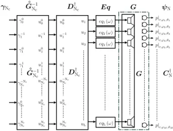
p|r,ϕ1,ϑ1 u0 0 u−1 1 u0 1 u1 1 u−Nc Nc u1 u2 u3 uL γ0 0 γ−1 1 γ0 1 γ1 1 γ−Nc Nc p|r,ϕ2,ϑ2 p|r,ϕM,ϑM D†Nc γNc G o −1 Nc G ψN eq1(ω) eq2(ω) eq3(ω) eqL(ω) u0 Nc uNc Nc γ0 Nc γNc Nc Eq G p|r,ϕ3,ϑ3 p|r,ϕ4,ϑ4 p|r,ϕ5,ϑ5 D†Nc CN† u0 0 u−1 1 u0 1 u1 1 u−Nc Nc u0 Nc uNc Nc Go−1 Nc

Figure 2: Block diagram of a spherical harmonics subspace directivity control (MIMO-SH-ctl).

Error Evaluation. To evaluate the system perfor-mance, spatial aliasing, i.e. all spherical harmonics N→

∞, needs to be taken into account. An ideal control system equals the identity matrix forn≤Nc, and zero

forn >Nc. The system errore(γNc) =E γNc depends

on the steering vector and is defined as deviation from this idealized behavior

E= GoNc Go>_Nc,Nc Go−1 Nc − INc 0>_Nc,Nc = 0Nc Go>_Nc,NcG o −1 Nc . (10) Following a similar approach as in [7], the minimum and maximum power of the error result from an eigendecom-position of the squared error, see also [18]

e(γNc) 2 =γ_NH_cEHE γNc, (11) EH_E=Qdiag{σe}2_QH_, ⇒argmin{σe}2≤ e(γNc) 2 γNc 2 ≤argmax{σe}2,

wherein ()H _{denotes hermitian transposition. As all}

eigenvectors inQare normalized, the magnitude of the squared error is determined by the eigenvalues only. The following sections apply the hereby defined error bounds and an average σe2

(Nc+1)2 to characterize the system

per-formance.

4

Case Study: Icosahedral

Loud-speaker

The IEM icosahedral array has a radius ofr_o= 0.28m and its 20 loudspeakers are built into an icosahedron with a common interior, loosely filled with damping wool.

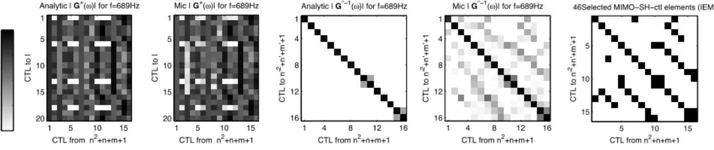
|g| in [dB] 0 −10 −20 −30 −40 Analytic | G+(ω)| for f=689Hz CTL to l CTL from n2_+n+m+1 1 5 10 15 1 5 10 15 20 Mic | G+(ω)| for f=689Hz CTL to l CTL from n2_+n+m+1 1 5 10 15 1 5 10 15 20

(a) MIMO-LSH-ctl at 689Hz, theoretical vs. practical

Analytic | G°−1(ω)| for f=689Hz CTL to n’ 2+n’+m’+1 CTL from n2_+n+m+1 1 4 8 12 16 1 4 8 12 16 Mic | G°−1(ω)| for f=689Hz CTL to n’ 2+n’+m’+1 CTL from n2_+n+m+1 1 4 8 12 16 1 4 8 12 16

(b) MIMO-SH-ctl at 689Hz, theoretical vs. practical

46Selected MIMO−SH−ctl elements (IEM)

CTL to n’ 2+n’+m’+1 CTL from n2+n+m+1 5 10 15 5 10 15 (c) Sparsification Mask

Figure 3: Cross-section through the MIMO-control systems for the IEM loudspeaker showing magnitudes at one frequency. The simulated systems are compared to measurement based control. The MIMO-SH-ctl becomes sparse in both cases.

4.1

Microphone Array Measurements

The measurement setup is depicted in Fig. 1 and uses a 10◦-spaced semicircular microphone array with 5◦offset fromϑ= 0. The transfer functions inGwere measured in 10◦azimuthal steps using an electric turntable. With the quadrature or surface fraction weightsw(cf. [1], [18]) for weighted least-squares inversion, the transfer func-tions were transformed from the left intoGc₁₇.

Furthermore, 20 filters have been applied to equalize all active on-axis loudspeaker responses to each other. This equalization step seems to be crucial for the sparse-ness of the MIMO-SH-ctl (see Figs. 2 and 3(b)).

From Gc₁₇, the MIMO-LSH-ctl Gc₃† and MIMO-SH-ctlGo₃−1were computed according the descriptions from above. In addition, analytic versions of the control sys-tems were calculated from the model in Appendix A.

Frequency Slice and Frequency Response. To il-lustrate the advantage of the MIMO-SH-ctl over the MIMO-LSH-ctl, a cross-section through the frequency-domain filter-matrix is depicted at a frequency of 689Hz. Figs. 3(a) and 3(b) compare the the analytic control systems to the corresponding systems based on mea-surements. It is nice to see that in both, theoretical and practical, results the MIMO-SH-ctl becomes sparse. However, the reason for the obvious deviation from the theoretical results is not quite clear yet (non-spherical geometry of the icosahedron; inhomogeneous filling and cabling in the interior; losses in the damping wool; slight offsets in the setup). The frequency responses of the

con-50 100 200 400 800 1600 −40 −20 0 20 40 60 f [Hz] |g ° +|[dB]_ij

Mic 16× 16 G°−1(ω)−Filters in SH domain

n=0 n=1 n=2 n=3 10↔11 15↔16

Figure 4: Measured MIMO-SH-ctl magnitude responses (thin, gray) from the IEM-loudspeaker in comparison to an-alytic responses (dashed, colored).

trol system Go−₃1 in magnitude are depicted in Fig. 4.

The dashed colored lines show the theoretical results; also here, the frequency responses from the measured data system (thin gray lines) deviate quite obviously from their analytical counterparts.

Making it Sparse again and Error Evaluation.

In order to re-establish a sparse structure in the MIMO-SH-ctl based on measurements, a mask needs to be found, omitting irrelevant transfer paths. Fig. 3(c) shows a se-lection of 46 important transfer functions. The error evaluation according to Eq. (11) in Fig. 5 shows a com-parison between the original and “sparsified” MIMO-SH-ctl. Even after a reduction from 256 to 46 transfer functions good results are achievable.

Figure 5: Synthesis errors of the IEM loudspeaker for N=3 comparing the full and the sparsified MIMO-SH-ctl. Results of the analytic model are given as reference.

4.2

Laser-Doppler Vibrometry

Measure-ments

Alternatively to the acoustic measurements, the vibra-tions of the membranes can be captured with a laser vibrometer [12, 13]. This is done with a much smaller measurement setup which is more robust to acoustic re-flections. However, laser vibrometry measurements only

|g| in [dB] 0 −10 −20 −30 −40 Analytic | T−1(ω)| for f=689Hz XTC to l’ XTC from l 1 5 10 15 20 1 5 10 15 20 LDV | T−1(ω)| for f=689Hz XTC to l’ XTC from l 1 5 10 15 20 1 5 10 15 20

(a) Velocity MIMO-ctl at 689Hz, theoretical vs. practical

Analytic | T°−1(ω)| for f=689Hz XTC to n’ 2+n’+m’+1 XTC from n2_+n+m+1 1 4 8 12 16 1 4 8 12 16 LDV | T°−1(ω)| for f=689Hz XTC to n’ 2+n’+m’+1 XTC from n2_+n+m+1 1 4 8 12 16 1 4 8 12 16

(b) Velocity MIMO-SH-ctl at 689Hz, theor./pract.

Figure 6: Cross-section through the velocity MIMO-control systems for the IEM loudspeaker showing magnitudes at one frequency. The simulated systems are compared to laser Doppler vibrometry measurement based control.

describe the surface velocity, but not the acoustic dis-persion. A spherical cap model (see Appendix A) was used to obtain sensible descriptions.

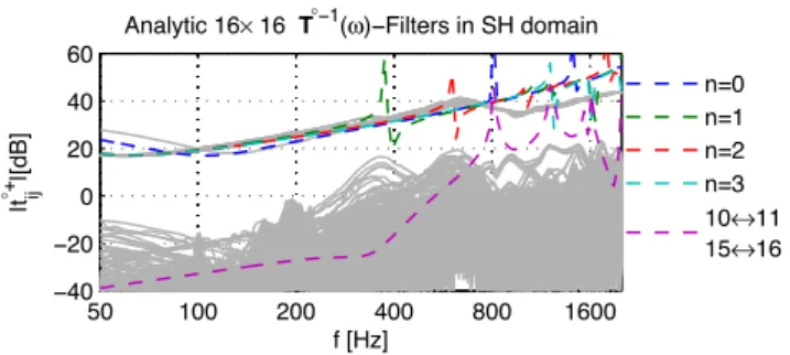
50 100 200 400 800 1600 −40 −20 0 20 40 60 f [Hz] |t ° +|[dB]_ij

Analytic 16× 16 T°−1(ω)−Filters in SH domain

n=0 n=1 n=2 n=3 10↔11 15↔16

Figure 7: Measured velocity MIMO-SH-ctl magnitude re-sponses (thin, gray) from the IEM-loudspeaker in compari-son to analytic responses (dashed, colored).

The description of the 20×20 velocity MIMO-system

T and its control is similar to the microphone array scenario

v =T u=T T−1vctl. (12)

The Nc-truncated spherical wave spectrum of the

sur-face velocity, using the spherical cap coefficientsA, cf. Ap-pendix A, and the decoderA†_Nc yields

ΥNc=A NcT A†Nc To_Nc

u=To_NcTo_N−1_c γNc. (13)

Fig. 6 compares a cross-section of the analytic con-trol system according to Appendix A with the laser vi-bromentry based system. The measured frequency re-sponses seem to match their analytic counterparts much better than in the case of microphone array measure-ments.

5

Conclusion

We have shown that control systems for angular beam-pattern synthesis can be made more efficient, at least for regular layouts of spherical loudspeaker arrays. The improvement, however, is not quite as good as could be expected from previous analytic simulations and a rea-sonable explanation for this has to be found. Neverthe-less, the computational effort can be decreased from 256 to 20+46 block-filters in case of the IEM loudspeaker.

6

Acknowledgements

The authors thank the University of Music and Dra-matic Arts Graz for granting a scholarship that intensi-fied the scientific exchange between IEM and CNMAT. We gratefully thank the Zukunftsfonds Steiermark (Prj. 3027) for supporting the research on spherical loudspeaker arrays. Adrian Freed has been a very encouraging dia-log partner in many interesting discussions. Thanks to Gottfried Behler’s remarks, the electro-acoustic model of spherical loudspeaker arrays could be improved.

References

[1] Sneeuw, N.: Global spherical harmonic analysis by least squares and numerical quadrature methods in historical perspective. Geophysical Journal Interna-tional, 1994.

[2] Warusfel, O.; Derogis, P.; Causs´e, R.: Radia-tion synthesis with digitally controlled loudspeakers, Proc. 103rd _{AES-Convention, New York, 1997.}

[3] Cook, P.; Essl, G.; Tzanetakis, G.; Trueman, D.: N>>2: Multi-speaker display systems for virtual re-ality and spatial audio projection. Proc. 5th _ICAD,

Glasgow, 1998.

[4] Trueman, D.; Bahn, C.; Cook, P.: Alternative voices for electronic sound. Proc. 140th _{ASA/NOISE joint}

meeting, 2000.

[5] Warusfel, O.; Misdariis, N.: From stage performance to domestic rendering. Proc. 116th_{AES Convention,}

Berlin, 2004.

[6] Kassakian, P.; Wessel, D.: Design of low-order filters for radiation synthesis. Proc. 115th_{AES-Convention,}

New York, 2003.

[7] Kassakian, P.; Wessel, D.: Characterization of spherical loudspeaker arrays. Proc. 117th

AES-Convention, San Francisco, 2004.

[8] Poletti, M.: Three-dimensional surround sound sys-tems based on spherical harmonics. AES Journal, vol. 53, no. 11, 2005.

[9] Lock, D.; Schiemer, G.; Ong, L.: Orbophone: A new interface for radiating sound and image. Proc. 12th

[10] Avizienis, R; Freed, A.; Kassakian, P.; Wessel, D.: A compact 120 independent element spherical loudspeaker array with programmable radiation pat-terns. Proc. 120th AES-Convention, Paris, 2006. [11] Behler, G.: Sound source for the measurement of

room impulse responses for auralization. Proc. 19th

ICA, Madrid, 2007.

[12] Reiner, P.; Jochum, C.: Measurement and evalua-tion of crosstalk within an icosehedral loudspeaker array. TI-Projekt, TU-Graz, Institut f¨ur Elektronis-che Musik und Akustik, http://iem.at, 2007. [13] Jochum, C.; Reiner, P.: Driving filters for

the icosahedral louspeaker array. TI-Projekt, TU-Graz, Institut f¨ur Elektronische Musik und Akustik, http://iem.at, 2007.

[14] Zotter, F.; H¨oldrich, R.: Modeling radiation syn-thesis with spherical loudspeaker arrays. Proc. 19th

ICA, Madrid, 2007.

[15] Zotter, F.; Noisternig, M.: Near- and farfield beam-forming using spherical loudspeaker arrays. Proc. 3rd

Congress, Alps Adria Acoustics Association, Graz, 2007.

[16] Pollow, M.: Variable directivity of dodecahedron loudspeakers. M. thesis, RWTH-Aachen, Institut f¨ur Technische Akustik, 2007.

[17] Zotter, F.; Schmeder, A.; Noisternig, M.: Crosstalk cancellation for spherical loudspeaker ar-rays. Fortschritte der Akustik, DAGA, Dresden, 2008.

[18] Pomberger, H.: Radial and angular directivity con-trol for spherical loudspeaker arrays. M. thesis, TU-Graz, Institut f¨ur Elektronische Musik und Akustik, 2008.

A

Analytic Model

The appendix provides a brief description completing the electro-acoustic model that has been previously be-gun in [14]. The analytic model is used as a reference to compare against measured data. Essentially, the acous-tical model has been given as a solid spherical shell with radially vibrating caps. The reader is referred to the pa-per [14] for a complete description. Let us resume at the description of the impact forcesfac_{of the acoustic fields}

on the loudspeaker membranes vibrating at the veloci-tiesv fac_=Zac_{·v, (14)} Zac_{= iρ} 0cATNdiagSH cin c jn(kinrin) j n(kinrin)+ hn(kro) h n(kro) AN (15) AN= SHT a(l)_(θ) l=1...L, (16)

whereina(l)_{is the aperture function defined to equal one}

at the coordinatesθ = (ϕ, θ) of thelth _{membrane and}

zero elsewhere. Let the matrix AN contain the

spher-ical harmonics coefficients vectors of all these aperture

functions. ()T_{denotes transposition,rinandrodescribe}

the inner and outer radius of the shell model, andkin, k, cin, and c the wave numbers and sonic speeds

in-side and outin-side the shell. jn and hn are the spherical

Bessel and Hankel functions,ρ0 is the air density, and i

the imaginary constant√−1.

i4 u4 u3 u2 u1 i3 i2 i1 v4 v3 v2 v1 f1 f2 f3 f4 zel l Rel l Lel l zme l ⎧ ⎨ ⎩ Rme l Sme l Mme l il=fl/βl ul=βlvl β1 β2 β3 β4 u,i zel _B f,v _zme _Zac

Figure 8: Complete electro-acoustical model of a spherical loudspeaker.

For the complete electro-mechanical model of the loudspeaker, the block diagram in Fig. 8 shows the rela-tion between electrical voltagesuand currentsiat the amplifier and the mechanical quantitiesf =fac_+fme

andv. The parameters correspond to electricalzel_,

me-chanicalzme, and acousticalZacimpedances, as well as the transduction (gyration) constants β. The relation between voltagesuand membrane velocitiesv yields

v=ZelB−1(Zac+Zme) +B−1

T

u, (17) with the diagonal matrices Zel = diagzel , Zme = diag{zme}, andB= diag{β}.

Using the radial propagation terms, the spherical wave-spectrum of the sound pressure results in

ψ=H ·AN·T Gc ·u, (18) H=iρ0cdiagSH hn(kr) h n(kro) (19) Eqs. (17) and (18) have been used to show the deviation of the practical results from the analytic model.