Estimation of the fuzzy reliability function using two-parameter exponential distribution as prior distribution

Vol. 8, No. 2, June 2020, pp.613-625

Estimation of the fuzzy reliability function using two-parameter

exponential distribution as prior distribution

Emad Hazem Abboudi1, Athraa Kamel Al – Mashhadani2, Muna Shaker Salman3 1_{Department of Statistics, University of Baghdad}

2_{Department of Accounting Techniques, Middle Technical University} 3_{Department of Computer Systems, Middle Technical University}

ABSTRACT

In this research, the fuzzy reliability function of the series system has been estimated using Bayes approach and Mellin transformation. It is based on the existence of two parameter exponential distribution as a previous distribution with the existence of a similar quadratic loss function, square loss function and non- asymmetric precautionary loss function. To apply the Bayes approach, the distribution parameters are assumed to be "random variables", and the traditional Bayes approach was used to obtain Bayes fuzzy capabilities by using Resolution Identity Theory in the fuzzy set. The simulation approach has been applied in this study to know the effect of α value on the fuzzy reliability function capabilities. The experiment has been carried out by assuming different values of the parameters as well as the sizes of the different samples. Furthermore, the applied part has dealt with the fuzzy reliability function estimation of both the quadratic loss function and the precautionary loss function with different α values using nonlinear membership functions. Some mathematical equations have been used to calculate the membership scores of the Bayes estimated points. This purpose has been achieved by converting the original problem into a non-linear programming problem and then divided it into eight secondary problems. The results have been obtained using the LINGO and GAMS programs.

Keywords: System reliability, Fuzzy environment, Bayes approach, Quadratic loss function, Precautionary loss function, Mellin transformation, Nonlinear programming

Corresponding Author Email:

Muna Shaker Salman, Computer Systems,

Middle Technical University,Iraq Email: [email protected] 1. Introduction

Our productive organization is currently facing a state of obsolescence in the process of the industrial bases modernization. Therefore, it is necessary to develop modern scientific methods to measure the "viability or aggravation of production machines by starting a scientific calculation of the efficiency of production machines through the use of a mathematical method for this purpose. That is the concept of reliability. So, the reliability of the machine has considered as one of the most important methods by knowing the ability of the machines to continuously work without a break for a certain period of time which may be long. Here, we observe a certain inaccuracy in determining the periods of time where the machines cease to work which in turn leads to the presence of fuzzy.

So, the estimation of the machine operation period is considered one of the phenomena in which its data has fuzzy property.

We note that specialists rely on the observation of the factors leading to the end of operational life of the machine under the most important environmental conditions. In fact, the machine may be aggravated during or after the specified period due to human errors or machine errors or some unexpected cases. Thus, the reliability function estimation for the machine represented by one year is a fuzzy number and therefore fuzzy set theory naturally offers a suitable tool for modeling the inaccurate models[6, 8, 4].

2. The theoretical side

This aspect is concerned with clarifying the fuzzy reliability function and some loss functions. Which are the quadratic loss function and the precautionary loss function. Thus, defining the reliability functions of the Series

system as well as deriving capabilities of the reliability function. Using the Bayes approach and Millen transformation method and using it in the "estimation process" by assuming that the distribution parameter is a random variable and is distributed according to the two parameter exponential distributions.

2.1. Fuzzy set

The fuzzy group

(A

̃)

upon the universal group

(𝑋̃)

is defined as classes of elements with a continuous membership.

[1, 2, 8]:

𝜇𝐴(𝑥) ∶ X → [0 ,1] (1)

2.2. Membership functions

The membership function is of "great importance" in the definition of "fuzzy set theory". It stands for functions by which the degree of membership of the element to the calculated fuzzy set[3, 13].

Theory (1): Let U is a universal group and Ṽ represents a partial fuzzy set belonging to the U group. The fuzzy set Ṽ has true membership function (t_Ṽ) and false membership function (fṼ) . Besides, tṼ: U → [0,1] fṼ: U →

[0,1] . Also t_Ṽ(U)+ f_Ṽ(U) ≤ 1 , and the t_Ṽ(u) could be represented as minimum of the true membership function

and f_Ṽ(𝑢) represents the minimum of the false membership function[3, 4, 5].

Theory (2): Let U = {u1, u2, … , un} , we can express the fuzzy set Ṽ derived from the group U as follows[2, 15] :

𝑉̃ = ∑𝑛_𝑖=1[𝑡_𝑉̃(𝑈), 1 − 𝑓_𝑉̃(𝑈)] 𝑢⁄ _𝑖 0 ≤ 𝑡_(𝑢𝑖) ≤ 1 − 𝑓_𝑉̃(𝑈) ≤ 1 ,i = 1,2, … , n (2) In other words, the period of membership (ui) is described as constrained within the period [t(ui), 1 − fṼ(ui)]

.The above membership function can be considered as generalization of the Trigonometric Membership Function which can be represented by the following formula:

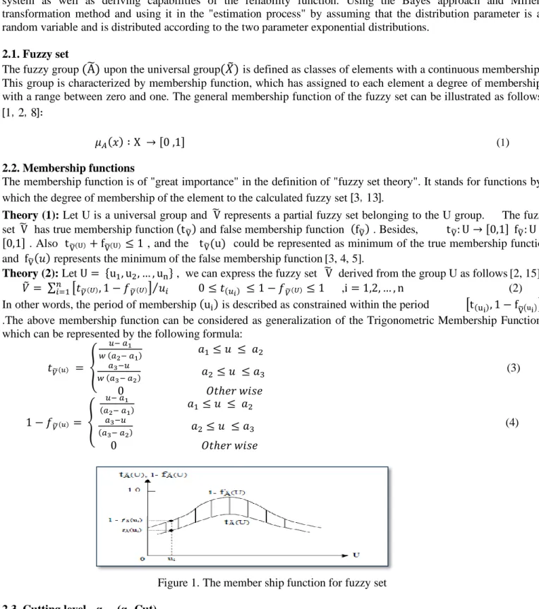
𝑡_𝑉̃(𝑢) = { 𝑢− 𝑎1 𝑤 (𝑎2− 𝑎1) 𝑎1≤ 𝑢 ≤ 𝑎2 𝑎3−𝑢 𝑤 (𝑎3− 𝑎2) 𝑎2 ≤ 𝑢 ≤ 𝑎3 0 𝑂𝑡ℎ𝑒𝑟 𝑤𝑖𝑠𝑒 (3) 1 − 𝑓_𝑉̃(𝑢) = { 𝑢− 𝑎1 (𝑎2− 𝑎1) 𝑎1≤ 𝑢 ≤ 𝑎2 𝑎3−𝑢 (𝑎3− 𝑎2) 𝑎2≤ 𝑢 ≤ 𝑎3 0 𝑂𝑡ℎ𝑒𝑟 𝑤𝑖𝑠𝑒 (4)

Figure 1. The member ship function for fuzzy set 2.3. Cutting level - α (α- Cut)

α is defined as the lowest degree of membership of any element in the fuzzy set Ṽ and the value of α falls within the closed period [0,1] [8].

Assuming that we have the set Ṽtv,_{̃ fṽ} , a partial fuzzy set is derived from the universal group U, which in turn possesses a valid membership function denoted by the symbol(tṽ). Invalid membership function is denoted by the

symbol (fṽ) . Through of what has been mentioned above, we can know αt− Cut and αf− Cut as in the

following formula[7, 17]:

𝑉̃𝛼𝑓= {𝑢: 𝑓𝑉̃(𝑢) ≥ 𝛼_𝑓} , 𝛼_𝑓 ∈ [0,1] (6) 2.4. Resolution identity for fuzzy sets

Assuming that Ṽtv,̃ fṽ is a "partial fuzzy set derived from the universal set" and U is characterized by having the true membership function and the false membership function as follows [15]:

𝑡_𝑉̃(𝑢)= sup 𝛼𝑡∈[0,1] 𝛼𝑡. I𝑉̃_𝛼𝑡(𝑢) , 0 ≤ 𝛼𝑡 ≤ 1 (7) 𝑓_𝑉̃(𝑢) = sup 𝛼𝑓∈[0,1] 𝛼𝑓. I𝑉̃_𝛼𝑓(𝑢) , 0 ≤ 𝛼𝑓 ≤ 1 (8) 2.5. Fuzzy reliability

Reliability is defined as" a measure of the viability or ability of any part of a particular system or system as a whole to function with complete validity without interruption". Or, it is defined as "the complementary function to the cumulative distribution function". It can be calculated from the probability of the machine survival after the expiry of a certain period of time and be "t" . The function of reliability is referred to as (R(t)) . The reliability function

could be expressed as follows [1, 14]: 𝑅(𝑡)= P(𝑇 > 𝑡)

= 1 − ∫ 𝑓(𝑡)𝑑𝑡 ₀𝑡

= 1 − 𝐹(t) (9)

But, in fact, the machine can stop working before the expiry of the specified time period. Some kinds of inaccuracy in knowing the time of machine stop lead to the presence of fuzzy in the time of the machine stop working which is symbolized by the symbol R̃(t) [8, 16].

𝑅̃(𝑡)= 𝑃(𝑇̃ >̃ 𝑡) (10(

Where 𝑇̃ >̃ 𝑡 ،𝑇̃ .

Note that T̃ has the function of failure 𝑓(𝑥̃) .and the function of membership𝑀(𝑥̃). Using the fuzzy probability

formula, we can calculate the fuzzy reliability of any machine in the system according to the following formula [13, 16]:

𝑅̃(𝑡)= ∫ 𝑀(𝑥̃)𝑓(𝑥̃) 𝑑(𝑥̃) ∞

𝑡 (11)

2.6. Systems reliability

The importance of reliability lies in attention to the internal relationships of the components of the system and the impact of these relationships on the reliability of the system as a whole. So, it is necessary to distinguish the type of system connection as series connection system, parallel connection system, and mixed connection system[7]. 2.7. Series system

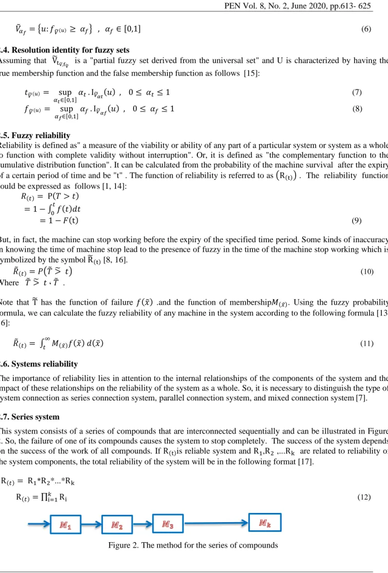
This system consists of a series of compounds that are interconnected sequentially and can be illustrated in Figure 2. So, the failure of one of its compounds causes the system to stop completely. The success of the system depends on the success of the work of all compounds. If R(t)is reliable system and R1,R2 ,...Rk are related to reliability of

the system components, the total reliability of the system will be in the following format [17]. R(𝑡)= R1*R2*...*Rk

R(𝑡)= ∏𝑘i=1Ri (12)

2.8. Mellin transformation

Mellin Transformation is an integral mathematical transformation through the differential equations transformed into mathematical equations. The probability density function of Mellin Transformation is given by the following formula[4, 17]:

M(f, u) = ∫ X∞ u−1_{f(x) dx}

0 (13)

Theory (1): Let x1, … , xk independent random variables have a probability density function 𝑓1, … , 𝑓𝑘 respectively,

and let g_k(y) be the probability density function of the random variable Y = ∏ki=1xi , we conclude that[6, 1]:

M(gk, u) = ∏ki=1M(fi , u) (14)

2.9. Fuzzy Bayes point estimation

Consider X is a random variable that has the probability density function, f(x|θ) and θ= (θ1, θ2, … , θn)

represents the parameter vector of (θ̃ ) and θ̃ = (θ̃_t1, θ̃t2, … , θ̃tn ; θ̃f1, θ̃f2, … , θ̃fn) is the vector of fuzzy

parameters for true and false membership functions. Each fuzzy parameter is associated with the membership function, Mt_Ṽ: θi→ [0,1] and MfṼ: θi→ [0,1]. Thus, the fuzzy parameters are θ̃i (θ̃iαt

L , θ̃i_αt U ; θ̃i_αf L , θ̃i_αf U ) and each αf ∈[0,1] and αt∈[0,1] to extract the Bayes digital estimators of the fuzzy parameters. These parameters

are assumed to be random variables having prior initial distributions based on the former experiences of available data. Based on initial distributions, Posture distributions are obtained. Thus, obtaining Bayes estimator is based on a specific loss function, so that we can find Bayes fuzzy points by the following [5, 16]:

𝑉𝛼𝑡 = [𝑚𝑖𝑛 { 𝑖𝑛𝑓 𝛼≤𝛽𝑡≤1𝜃̃̂𝛽𝑡 𝐿 _{, 𝑖𝑛𝑓} 𝛼≤𝛽𝑡≤1𝜃̃̂𝛽𝑡 𝑈_{} , 𝑚𝑎𝑥 { 𝑠𝑢𝑝} 𝛼≤𝛽𝑡≤1𝜃̃̂𝛽𝑡 𝐿 _{, 𝑠𝑢𝑝} 𝛼≤𝛽𝑡≤1𝜃̃̂𝛽𝑡 𝑈_{}] (15)} 𝑉𝛼𝑓 = [𝑚𝑖𝑛 { 𝑖𝑛𝑓 𝛼≤𝛽𝑓≤1𝜃̃̂𝛽𝑓 𝐿 _{, 𝑖𝑛𝑓} 𝛼≤𝛽𝑓≤1𝜃̃̂𝛽𝑓 𝑈 _{} , 𝑚𝑎𝑥 { 𝑠𝑢𝑝} 𝛼≤𝛽𝑓≤1𝜃̃̂𝛽𝑓 𝐿 _{, 𝑠𝑢𝑝} 𝛼≤𝛽𝑓≤1𝜃̃̂𝛽𝑓 𝑈_{}] (16)}

Note that equation (15) and (16) contain all Bayes' estimated fuzzy points. 2.10. Loss functions

In order to obtain the Bayes estimates, you must determine the loss function that affects the determination of the Bayes estimator. There are several types of loss functions including the quadratic loss function. This stands for a symmetrical loss function. It means that the amount of loss allocated to the positive false is equal to the negative false for the same amount and is considered one of the most important functions of loss in the statistical estimates of Bayes given according to non-symmetric precautionary loss function as follows[10, 11]:

𝜃̂𝑝2= 𝐸(𝜃2|𝑡) (17)

For the precautionary asymmetric loss function, it will be according to the following formula:

𝐿(𝜃̂, 𝜃) =(𝜃̂ −𝜃)

2

𝜃̂𝜃 (18)

2.11. Method of the fuzzy reliability function estimation

Assuming we have a sequential system consisting of k of independent compounds and that the lifetime distribution for each compound follows the exponential distribution. On other words, the reliability function at time (t) is

R(𝑡) = e−λt _{and (λ) is a failure rate[6].}

Assuming we have t1,t2, … … , tn which represents the failure times during the test period, and the test duration

for each compound is independent and symmetrical with the exponential distributionT1≤ T2≤ ⋯ ≤ Tk , the total

duration of the test is given in the following formula [5]:

𝑇. 𝑇 = ∑𝑘𝑖=1(𝑇𝑖𝑗) + (𝑛𝑖− 𝑚𝑖) 𝑇(𝑚𝑖) (19)

By substituting V for the total run time (T.T) and to apply the Bayes approach, the failure rate must be random variable Ʌ having the exponential distribution with two parameters as the previous distribution 𝐸(𝜃𝑖1, 𝜃𝑖2) with

the probability density function shown below[17]:

π Ʌ(𝜆i) = θi2e−θi2(λi−θi1) λ ≥ θi1 (20)

So, 𝜃𝑖1, 𝜃𝑖2 represent both as parameter of form and scale parameter, respectively.

Assuming that the random variable Ʌ𝑖=Ʌ𝑖- θi1 has the exponential distribution as the prior distribution given by the

π Ʌ(𝜆i) = θie−θi λi λ𝑖 ≥ 0 (21)

h(𝑚|𝜆) = 𝑓(𝑚|λ)πɅ(𝜆)

∫₀∞𝑓(𝑚|y)πɅ(λ_i) 𝑑𝑦 (22)

And by replacing the equation 20 and 21 with the equation 22, we obtain:

h(λ|m, 𝑡) =(t𝑖+θ )m𝑖+1

Γ_(m𝑖+1) λ

m𝑖_e−λ(t+ θ) ₍₂₃₎ The value t could be compensated with total run time V and it could obtain the following[13]:

∴ ℎ(𝑚|λ) ~ 𝐺𝑎𝑚𝑚𝑎 (𝑚𝑖+ 1 , 𝑡 + 𝜃)

Since the reliability function r(𝑡) = e−λθ _{is described as a decreasing monotonous function of (λ). This indicates}

that there is a relationship (one –to- one) between (r) and (λ) Therefore, There is a single inverse given by the following relationship [13]:

𝜆 = − 𝐿𝑛 (r)_(𝑡) , 0 ≤ r ≤ 1 , 𝑡 > 0 (24) Since the probability density function of 𝑅 = R (𝑡) and for any constant value of t is given by the following formula, we get: 𝜋𝑅(𝑟) = 𝜋Ʌ (−𝐿𝑛 𝑟 𝑡 ) | 𝑑𝜆 𝑑𝑟| = 𝜋Ʌ (−𝐿𝑛 𝑟 𝑡 ) ( 1 𝑟∗𝑡) = ( 𝜃𝑖 𝑡𝑖) (25) 𝜋𝑅(𝑟) = 𝜋Ʌ [−𝐿𝑛 𝑟 𝑡 ] [ 1 𝑟∗𝑡]

Thus, the formula above is used to find the prior distribution or the posture distribution of (R). And now according to equation (20) and (25), we get the prior distribution of (R) according to the following formula[5]:

𝜋𝑅(𝑟) = 𝜋Ʌ (−𝐿𝑛 𝑟 𝑡 ) [ 1 𝑟∗𝑡] = ( 𝜃𝑖 𝑡𝑖) ∗ 𝑟𝑖 𝜃/𝑡 ₍₂₆₎

It is described as having 𝑁𝑒𝑔𝑎𝑡𝑖𝑣𝑒 − 𝐿𝑜𝑔 − 𝐺𝑎𝑚𝑚𝑎 (𝑚𝑖+ 1 , ((𝑡 + 𝜃)𝑖⁄ )𝑡𝑖 when (m) has a state of failure

during the period (V). According to equation (23), the posterior distribution of (Ʌ) is 𝐺𝑎𝑚𝑚𝑎 (𝜃1+ 𝑚 , 𝑉 + 𝜃2).

By using equation (25) again, the posterior distribution of (R) is 𝑁𝑒𝑔𝑎𝑡𝑖𝑣𝑒 𝐿𝑜𝑔 − 𝐺𝑎𝑚𝑚𝑎 (𝑚𝑖+

1 , ((𝑡 + 𝜃)𝑖⁄ )𝑡𝑖 given in the following form [6, 5,9]:

𝜋𝑅(𝑟|𝑚, 𝑣) = [(𝑣+ 𝜃𝑖) 𝑡⁄ ]𝑚+1 . 𝑟𝑖(𝑣+𝜃𝑖)𝑡𝑖−1 . (−𝐿𝑛 𝑟)𝑚𝑖

Γ_(𝑚𝑖+1) 0 ≤ 𝑟 ≤ 1 (27)

By equation (27) and by introducing the probability density function of the Mellin transformation and the posterior function of 𝑅𝑖 and by making integrals, we get[6, 5]:

𝑀(𝜋𝑅(𝑟|𝑚, 𝑣); 𝑢) = ( 𝑣+𝜃𝑖

𝑣𝑖+𝜃𝑖+(𝑢−1)∗𝑡𝑖)

𝑚𝑖+1

(28) Since we have a series system composed of (k) independent compounds, the reliability of the serial system is the result of multiplying the reliability of the compounds within the system. On other words, 𝑅 = ∏𝑘𝑖=1𝑅𝑖 and through

equation (14) and equation (28). The probability density function of the posteri or distribution of system reliability R is at time t and ((𝑡𝑖 = 𝑡 , 𝑖 = 1, … , 𝑘) .[8,15] 𝑀(𝜋𝑅(𝑟|𝑚, 𝑣); 𝑢) = ∏ ( 𝑣+𝜃𝑖 𝑣+𝜃_𝑖+(𝑢−1)𝑡) 𝑚+1 𝑘 𝑖=1 (29)

With a quadratic loss function, the estimated fuzzy point of the system reliability is the mean of the Posterior distribution [1, 9]: ∴ 𝑟̂𝑆= 𝐸[(𝑟|𝑚, 𝑣)] = 𝑀(𝜋𝑅(𝑟|𝑚, 𝑣); 𝑢 = 2) = ∏ ( 𝑣+𝜃𝑖 𝑣+𝜃𝑖+𝑡) 𝑚_𝑖+1 𝑘 𝑖=1 (30)

With a protective loss function, the Bayes' estimated fuzzy point of system reliability is the posterior distribution mean [9]: 𝑟̂𝑝 = (𝐸[(𝑅2|𝑚, 𝑣)]) 1 2 ⁄ _{= [𝑀(𝜋𝑅(𝑟|𝑚, 𝑣); 𝑢 = 3)]}1⁄_{2= ∏ (} 𝑣+𝜃𝑖 𝑣+𝜃𝑖+2𝑡) (𝑚𝑖+1) 2 ⁄ 𝑘 𝑖=1 (31)

By using one of the fuzzy numbers, we can rewrite the fuzzy time in the following format: [13]

"

𝑇. 𝑇

̃

=

[



𝑡̃

]



)

1̂



𝑇̂

(

Bayes' fuzzy point of system reliability could be obtained for both true membership function and false membership function with quadratic loss function and precautionary loss function given in the following formula [4, 5, 9]:

(R̂s)αtL = ∏ [ ∑mj=1(t̃F)Lαt+(ni−mi)(t̂imi)αtL+(θi)αtL ∑mj=1(t̃F)αtL+(ni−mi)(t̂imi)αtL+(θi)αtL+T ] mi+1 k i=1 (R̂s)αtU = ∏ [ ∑mj=1(t̃F)Uαt+(ni−mi)(t̂imi)αtL+(θi)αtU ∑mj=1(t̃F)αtU+(ni−mi)(t̂imi)αtU+(θi)αtU+T ] m_i+1 k i=1 ( 33) (R̂p)αtL = ∏ [ ∑mj=1(t̃F)Lαt+(ni−mi)(t̂imi)αtL+(θi)αtL ∑mj=1(t̃F)αtL+(ni−mi)(t̂imi)αtL+(θi)αtL+2T ] mi+1 2 ⁄ k i=1 (R̂p)αtU = ∏ [ ∑mj=1(t̃F)Uαt+(ni−mi)(t̂imi)αtL+(θi)αtU ∑mj=1(t̃F)αtU+(ni−mi)(t̂imi)αtU+(θi)αtU+2T ] m_i+1 2 ⁄ k i=1 ( 34)

Four each α∈[0,1] it is:

"𝑉(𝑅)𝛼𝑡 = [𝑚𝑖𝑛 { min 𝛼≤𝛽≤1𝑟̃̂𝛽 𝐿_{, min} 𝛼≤𝛽≤1𝑟̃̂𝛽 𝑈_{} , 𝑚𝑎𝑥 { max} 𝛼≤𝛽≤1𝑟̃̂𝛽 𝐿_{, max} 𝛼≤𝛽≤1𝑟̃̂𝛽 𝑈_{}] (35)}

For used false member ship function, the estimate will be as follows [9, 5]:

(R̂s)αfL = ∏ [ ∑mj=1(t̃F)Lαf+(ni−mi)(t̂imi)αfL+(θi)αfL ∑mj=1(t̃F)αfL+(ni−mi)(t̂imi)αfL+(θi)αfL+T ] m_i+1 k i=1 (R̂s)αfU = ∏ [ ∑mj=1(t̃F)Uαf+(ni−mi)(t̂imi)αfL+(θi)αfU ∑mj=1(t̃F)αfU+(ni−mi)(t̂imi)αfU+(θi)αfU+T ] m_i+1 k i=1 (36) (R̂p)αfL = ∏ [ ∑mj=1(t̃F)Lαf+(ni−mi)(t̂imi)αfL+(θi)αfL ∑mj=1(t̃F)αfL+(ni−mi)(t̂imi)αfL+(θi)αfL+2T ] m_i+1 2 ⁄ k i=1 (R̂p)αfU = ∏ [ ∑mj=1(t̃F)Uαf+(ni−mi)(t̂imi)αfL+(θi)αfU ∑mj=1(t̃F)αfU+(ni−mi)(t̂imi)αfU+(θi)αfU+2T ] m_i+1 2 ⁄ k i=1 ( 37) And: "𝑉(𝑅)𝛼𝑓= [𝑚𝑖𝑛 { min 𝛼≤𝛽≤1𝑟̃̂𝛽 𝐿_{, min} 𝛼≤𝛽≤1𝑟̃̂𝛽 𝑈_{} , 𝑚𝑎𝑥 { max} 𝛼≤𝛽≤1𝑟̃̂𝛽 𝐿_{, max} 𝛼≤𝛽≤1𝑟̃̂𝛽 𝑈_{}] (38)}

Note that equation (35) and equation (38) contain all points of the Bayes estimators for each 𝑟 ∈ [𝑟̃𝛼𝑡𝐿 , 𝑟̃𝛼𝑡𝐿 ]

[𝑟̃_𝛼𝑓𝐿 _{, 𝑟̃}

𝛼𝑓𝐿 ] and that the membership function of Bayes' estimated fuzzy points of the reliability 𝒓̃ at the time t is

denoted by the symbol 𝒓̃̂ and is defined by the following formula[6]:

𝑀_𝒓̃̂(𝑟) = Sup

0≤𝛼≤1𝐼𝑉(𝛼)

(𝑟) (39)

2.12. Computational procedures for the non-linear programming method

The Computational procedures are presented to evaluate or calculate the true and false membership of Bayes ' s estimated fuzzy points given in equation (15) and equation (16). By adopting equation (35) and (38) with the following symbols, we get[8]:

𝑉∝𝑡= [𝑔(𝛼𝑡) , "ℎ (𝛼𝑡)] = [min{𝑔1(𝛼𝑡), 𝑔2(𝛼𝑡)} , max{ℎ1(𝛼𝑡), ℎ2(𝛼𝑡)}]" (39) 𝑉∝𝑓 = [𝑔(𝛼𝑓) , ℎ (𝛼𝑓)] = [" min {𝑔 1(𝛼𝑓), 𝑔2(𝛼𝑓)} , max {ℎ1(𝛼𝑓), ℎ2(𝛼𝑓)}] " (40) and, 𝑔₂(𝛼𝑡) = inf 𝜃̃̂𝐵𝑡𝑈 𝛼𝑡≤𝐵𝑡≤1 𝑔₁(𝛼𝑡) = inf 𝜃̃̂𝐵𝑡𝐿 𝛼𝑡≤𝐵𝑡≤1 "ℎ₂(𝛼𝑡) = sup 𝜃̃̂𝐵𝑡𝑈 𝛼𝑡≤𝐵𝑡≤1 " ℎ₁(𝛼𝑡)= " sup 𝜃̃̂𝐵𝑡𝐿 𝛼𝑡≤𝐵𝑡≤1 " "𝑔 2(𝛼𝑓) = inf 𝜃̃̂𝐵𝑓 𝑈 𝛼𝑓≤𝐵𝑓≤1 " "𝑔 1(𝛼𝑓) = inf 𝜃̃̂𝐵𝑓 𝐿 𝛼𝑓≤𝐵𝑓≤1 " "ℎ 2(𝛼𝑓) = sup 𝜃̃̂𝐵𝑓 𝑈 𝛼𝑓≤𝐵𝑓≤1 " "ℎ 1(𝛼𝑓) = sup 𝜃̃̂𝐵𝑓 𝐿 ∝_𝑓≤𝐵_𝑓≤1 "

Based on equation (7) and (8), the true membership function and the false membership function of the Bayes' fuzzy estimators 𝜃̃̂ are given by the following formula [9]:

𝑡_𝜃̂̃(𝑟) = sup 𝛼𝑡 𝛼𝑡∈ [0,1] . I(𝑉𝛼𝑡)(𝑟) = sup{𝛼𝑡 : 𝑔(𝛼𝑡) ≤ 𝑟 ≤ ℎ(𝛼𝑡) , 0 ≤ 𝛼𝑡 ≤ 1 } (41) 𝑓_𝜃̂̃(𝑟) = sup 𝛼𝑓 𝛼𝑓∈ [0,1] . I_(𝑉 𝛼𝑓)(𝑟) = sup {𝛼𝑓 : 𝑔(𝛼_𝑓) ≤ 𝑟 ≤ ℎ(𝛼𝑓) , 0 ≤ 𝛼𝑓 ≤ 1 } (42)

max 𝛼𝑓 s.t min{𝑔1(𝛼𝑓) , 𝑔2(𝛼𝑓)} ≤ 𝑟 max{ℎ1(𝛼𝑓) , ℎ2(𝛼𝑓)} ≥ 𝑟 0 ≤ 𝛼𝑓 ≤1 max 𝛼𝑡 s.t "min{𝑔1(𝛼𝑡) , 𝑔2(𝛼𝑡)} ≤ 𝑟" "max{ℎ1(𝛼𝑡) , ℎ2(𝛼𝑡)} ≥ 𝑟" 0 ≤ 𝛼𝑡≤ 1

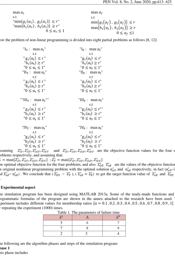
Now the problem of non-linear programming is divided into eight partial problems as follows [8, 12]: "IT : max αt" s.t " g1(αt) ≤ r " "h1(αt) ≥ r" "0 ≤ αt≤ 1" "IIT : max αt" s.t " g1(αt) ≤ r " "h2(αt) ≥ r" "0 ≤ αt≤ 1" ""IIIT : max αt"" s.t " g2(αt) ≤ r " "h1(αt) ≥ r" "0 ≤ αt≤ 1" "IVT : max αt" s.t "g2(αt) ≤ r" "h2(αt) ≥ r" "0 ≤ αt≤ 1" "IF : max αf" s.t "g1(αf) ≤ r" "h1(αf) ≥ r" "0 ≤ αf ≤ 1" "IIF : max αf" s.t "g1(αf) ≤ r" "h2(αf) ≥ r" "0 ≤ αf ≤ 1" "IIIF : max αf" s.t ""g2(αf) ≤ r"" "h1(αf) ≥ r" "0 ≤ αf ≤ 1" "IVF : max αf" s.t "g2(αf) ≤ r" "h2(αf) ≥ r" "0 ≤ αf ≤ 1"

Assuming 𝑍𝐼𝑇∗ , 𝑍𝐼𝐼𝑇∗ , 𝑍𝐼𝐼𝐼𝑇∗ , 𝑍𝐼𝑉𝑇∗ and 𝑍𝐼𝐹∗ , 𝑍𝐼𝐼𝐹∗ , 𝑍𝐼𝐼𝐼𝐹∗ , 𝑍𝐼𝑉𝐹∗ are the objective function values for the four

sub-problems respectively, and assuming that:

𝑍_𝑇∗ _{= max{𝑍}

𝐼𝑇∗ , 𝑍𝐼𝐼𝑇∗ , 𝑍𝐼𝐼𝐼𝑇∗ , 𝑍𝐼𝑉𝑇∗ } ; 𝑍𝐹∗= max{𝑍𝐼𝐹∗ , 𝑍𝐼𝐼𝐹∗ , 𝑍𝐼𝐼𝐼𝐹∗ , 𝑍𝐼𝑉𝐹∗ }

The optimal objective function for the four problems, and also ZOT∗ ZoF∗ are the values of the objective function of

the original nonlinear programming problem with the optimal solution αoT∗ and αoF∗ respectively, in fact (αoT∗ =ZOT∗

and Z_oF∗ _=α oF

∗ _{(. We conclude that ( Z} OT ∗ _{= Z}

T∗ ), ( ZoF∗ = Z∗F) to get the target function value of ZoF ∗ and ZOT∗ [5,

6].

3. Experimental aspect

The simulation program has been designed using MATLAB 2013a. Some of the ready-made functions and the programmatic formulas of the program are shown in the annex attached to the research have been used. The experiment includes different values for membership ratios [α = 0.1 , 0.2 , 0.3 , 0.4 , 0.5 , 0.6 , 0.7 , 0.8 , 0.9 , 1] and by repeating the experiment (1000) times.

Table 1. The parameters of failure time

λ𝑈 Λ λ𝐿 7 6 5 9 8 7 4 3 2

The following are the algorithm phases and steps of the simulation program: Phase 1

1. Random values are selected for failure parameters. Then, the value of the cutting is added and subtracted to get three sets of parameters through which data for the program is to be generated.

2. The sample size and the number of machines under study are defined. Three different sample sizes have been selected in each iteration.

N= 50, 100, 120

3. The number of iterations of the experiment (L = 1000), as well as the reservoirs for the results and for each value are determined.

Phase 2

This phase includes

1. Data on failure times are generated according to the exponential distribution and depending on the parameters generated in the first stage.

2. Cutting is determined for failure times as well as for parameters of the generated data. Phase 3

1. At this point the value of cutting is defined and the values [α = 0.1, 0.2, 0.3, 0.4, 0.5, 0.6, 0.7, 0.8, 0.9, 1]. 2. The value of cutting is commutated concerning with the failure times as well as for parameters at ratio 1%. Phase 4

In this stage, the cutting level for data generated above is computed by adding the minimum of the denominator of the membership function, and subtracting the maximum to the denominator of the membership function and for both the true and false membership function.

Phase 5

This phase includes:

1. The reliability function of each machine and the system as a whole is calculated by having a quadratic loss function, a precautionary loss function and for each value of α value using the true and false membership function 2.The lowest value is to be selected from the minimum values and higher value from the maximum values for the estimated reliability function by the presence of quadratic loss function and precautionary loss function using the true membership function and false membership function.

3. After a repetition of the experiment (L = 1000), the arithmetic mean of the results is calculated for each α and for each repetition.

4. The value of α. which corresponds to the best value of the reliability function is derived by the presence of both loss functions.

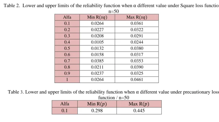
Table 2. Lower and upper limits of the reliability function when α different value under Square loss function / n=50

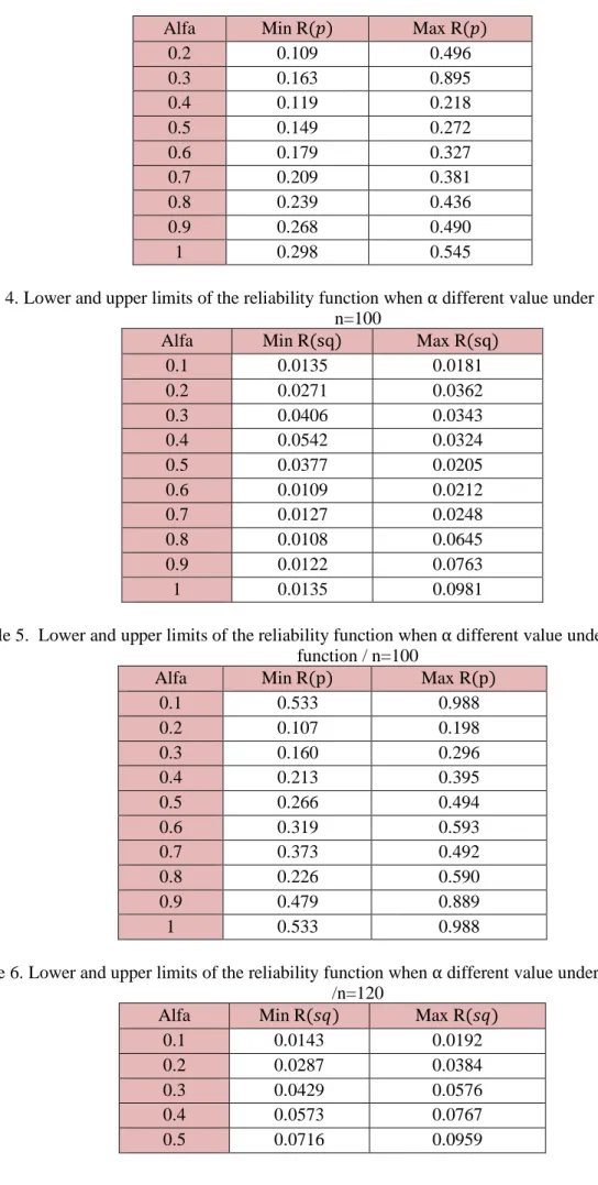
Table 3. Lower and upper limits of the reliability function when α different value under precautionary loss function / n=50

Alfa Min R(𝑝) Max R(𝑝)

0.1 0.298 0.445

Alfa Min R(𝑠𝑞) Max R(𝑠𝑞)

0.1 0.0264 0.0361 0.2 0.0227 0.0322 0.3 0.0208 0.0291 0.4 0.0105 0.0244 0.5 0.0132 0.0380 0.6 0.0158 0.0317 0.7 0.0385 0.0353 0.8 0.0211 0.0390 0.9 0.0237 0.0325 1 0.0264 0.0461

Alfa Min R(𝑝) Max R(𝑝) 0.2 0.109 0.496 0.3 0.163 0.895 0.4 0.119 0.218 0.5 0.149 0.272 0.6 0.179 0.327 0.7 0.209 0.381 0.8 0.239 0.436 0.9 0.268 0.490 1 0.298 0.545

Table 4. Lower and upper limits of the reliability function when α different value under Square loss function / n=100

Alfa Min R(sq) Max R(sq)

0.1 0.0135 0.0181 0.2 0.0271 0.0362 0.3 0.0406 0.0343 0.4 0.0542 0.0324 0.5 0.0377 0.0205 0.6 0.0109 0.0212 0.7 0.0127 0.0248 0.8 0.0108 0.0645 0.9 0.0122 0.0763 1 0.0135 0.0981

Table 5. Lower and upper limits of the reliability function when α different value under precautionary loss function / n=100

Alfa Min R(p) Max R(p)

0.1 0.533 0.988 0.2 0.107 0.198 0.3 0.160 0.296 0.4 0.213 0.395 0.5 0.266 0.494 0.6 0.319 0.593 0.7 0.373 0.492 0.8 0.226 0.590 0.9 0.479 0.889 1 0.533 0.988

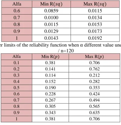
Table 6. Lower and upper limits of the reliability function when α different value under Square loss function /n=120

Alfa Min R(𝑠𝑞) Max R(𝑠𝑞)

0.1 0.0143 0.0192

0.2 0.0287 0.0384

0.3 0.0429 0.0576

0.4 0.0573 0.0767

Alfa Min R(𝑠𝑞) Max R(𝑠𝑞) 0.6 0.0859 0.0115 0.7 0.0100 0.0134 0.8 0.0115 0.0153 0.9 0.0129 0.0173 1 0.0143 0.0192

Table 7. Lower and upper limits of the reliability function when α different value under precautionary loss function / n=120

Alfa Min R(𝑝) Max R(𝑝)

0.1 0.381 0.706 0.2 0.141 0.762 0.3 0.114 0.212 0.4 0.152 0.282 0.5 0.190 0.353 0.6 0.228 0.424 0.7 0.267 0.494 0.8 0.305 0.565 0.9 0.343 0.635 1 0.381 0.706 4.Application side

Al-Fatah plant of the General Company for Woolen Industries, which is one of the Ministry of Industry and Minerals formations, has been chosen as the place of application of the study. The plant consists of the following sections (wool and tanning department, spinning section and combed spinning section textile department. The machines of the textile department have been selected as one of the main sections in the factory and include a variety of products (blankets, carpets and fabrics). Data has been collected from the blankets production machines for the purpose of analyzing and estimating their reliability. Note that the method of linking the production lines systems of the textile department is a serial link. The production line for the manufacture of blankets has been chosen as a place to collect data related to the research. The factory operates (7 hours per day). By collecting data and information about the blanket production line machines belonging to the General Company for Wool Industries, the downtime of the production line machines has been obtained as shown in Table 8. The failure time parameters have been obtained using (Easy –Professional 5.5. Fit) and as shown in Table 8.

Table 8. The data of each number of test cases and number of failures as well as the failure time for each composition in addition to the parameters of failure time

Unit tested Test terminated at

m th failure Failure time (h)

Parameter of Failure time

Component 1 4 2 4̃ , 6̃ 6̂

Component 2 4 3 5̂, 7̂ , 3̂ 8̂

Component 3 3 1 6̂ 3̂

The membership function is calculated for each of the failure times as well as the parameters according to the formula (3 and 4) as shown below:

t₈̃= { u−7 2 , 7 ≤ u ≤ 8 9−u 2 , 8 ≤ u ≤ 9 1 − f₈̃= { u−7 1 , 7 ≤ u ≤ 8 9−u 1 , 8 ≤ u ≤ 9 t7̃= { u−6 2 , 6 ≤ u ≤ 7 8−u 2 , 7 ≤ u ≤ 8 1 − f7̃= { u−6 1 , 6 ≤ u ≤ 7 8−u 1 , 7 ≤ u ≤ 8

To obtain the reliability of the Bayes Fuzzy system, initially α− Cutt and α− Cutf are extracted for fuzzy

numbers as shown below:

8̃𝛼𝑡 = [7 + 2𝛼𝑡 , 9 − 2𝛼𝑡] 8̃𝛼𝑓 = [7 + 1𝛼𝑓 , 9 − 1𝛼𝑓]

7̃𝛼𝑡= [6 + 2𝛼𝑡 , 8 − 2𝛼𝑡] 7̃𝛼𝑓 = [6 + 1𝛼𝑓 , 8 − 1𝛼𝑓]

Thus, the reliability function of the system is estimated using the true membership function. and both the quadratic loss function and the precautionary loss function according to formula (33) and (34) respectively:

R̂̃(𝑠𝑞)_αtL _{= [}(25+10αt) (32+10αt)] 3 ∗ [(20+10αt) (27+10αt)] 4 ∗ [(20+8αt) (27+8αt)] 2 R̂̃(𝑠𝑞)αtU = [ (35−10αt) (42−10αt)] 3 ∗ [(30−10αt)_(37−10αt)]4∗ [_{(35−8 αt)}(28−8αt)]2 R̂̃(𝑃)_αtL _{= [}(25+10αt) (39+10αt)] 2 ∗ [(20+10αt)_(34+10αt)]3∗ [(20+8αt)_(34+8αt)]2 R̂̃(P)αtU = [ (35−10αt) (49−10αt)] 2 ∗ [(30−10αt)_(44−10αt)]3∗ [_{(42−8 αt)}(28−8αt)]2

The estimators of the reliability function of the system are based on false membership function and for both the quadratic loss function and the precautionary loss function according to formula (36) and (37) respectively.

R ̂ ̃(𝑠𝑞)_α𝑓L _{= [}(25+5α𝑓) (32+5α𝑓)] 3 ∗ [(20+5α𝑓)_(27+5α𝑓)]4∗ [(20+4 α𝑓)_{(27+4 α𝑓)}]2 R ̂ ̃(𝑠𝑞)_α𝑓U _{= [}(35−5α𝑓) (42−5α𝑓)] 3 ∗ [(30−5α𝑓)_{(37−5α𝑓)}]4∗ [(28−4 α𝑓)_{(35−4 α𝑓)}]2 R ̂ ̃(P)_αfL _{= [}(25+5αf) (39+5αf)] 2 ∗ [(20+5αf)_(34+5αf)]3∗ [(20+4αf)_(34+4αf)]2 R̂̃(P)_αfU = [(35−5 αf)_{(49−5 αf)}]2∗ [(30−5αf)_(44−5αf)]3∗ [(28−4 αf)_{(42−4 αf)}]2

When compensating for 𝛼𝑡 = 0.5, we get:

(𝑟̃̂)

0.5 𝐿

= (0.1299) = (𝑟̃̂)_0.5𝑈 In other words, 𝑡_𝑟̃̂(0.1299) = 0.5

On the other hand, when compensating for 𝛼𝑓 = 1 , we get (𝑟̃̂)₁ 𝐿

= (0.1299) = (𝑟̃̂)₁𝑈

In other words, 1 − 𝑓_𝑟̃̂(0.1299) = 0.87

And that 𝐴𝑜= [0.014 , 0.219]

If the value of the reliability function belongs to the period𝑟 ∈ 𝑉𝑜, we can make calculations for the following cases

to find the proportion of membership:

- If r <0.1299, we can solve the problem of non-linear programming using LINGO software. 𝑡_𝑟̃̂(𝑟) = 𝑚𝑎𝑥 {𝛼𝑡 ∈ [0,1] ∶ 𝑔(𝛼𝑡) = 𝑔1(𝛼𝑡) = (𝑟̃̂)_𝛼𝑡 𝐿 } = [(25+10αt)_(32+10αt)]3∗ [(20+10αt)_(27+10αt)]4∗ [(20+8αt)_(27+8αt)]2≤ 𝑟 = [(25+10αt)_(39+10αt)]2∗ [(20+10αt)_(34+10αt)]3∗ [(20+8αt)_(34+8αt)]2 ≤ 𝑟 1 − 𝑓_𝑟̃̂(𝑟)

= 𝑚𝑎𝑥 {𝛼𝑓 ∈ [0,1] ∶ 𝑔(𝛼𝑓) = 𝑔1(𝛼𝑓) = (𝑟̃̂)_𝛼𝑓 𝐿 } = [(25+5α𝑓)_(32+5α𝑓)]3∗ [(20+5α𝑓)_(27+5α𝑓)]4∗ [(20+4 α𝑓)_{(27+4 α𝑓)}]2≤ 𝑟 = [(25+5𝛼𝑓) (39+5𝛼𝑓)] 2 ∗ [(20+5𝛼𝑓) (34+5𝛼𝑓)] 3 ∗ [(20+4𝛼𝑓) (34+4𝛼𝑓)] 2 ≤ 𝑟 - If r> 0.1299, we solve the following problem:

𝑡_𝑟̃̂(𝑟) = 𝑚𝑎𝑥 {𝛼𝑡 ∈ [0,1] ∶ 𝑔(𝛼𝑡) = 𝑔1(𝛼𝑡) = (𝑟̃̂)_𝛼𝑡 𝐿 } = [(25+10αt)_(32+10αt)]3∗ [(20+10αt)_(27+10αt)]4∗ [(20+8αt)_(27+8αt)]2≥ 𝑟 = [(25+10αt)_(39+10αt)]2∗ [(20+10αt)_(34+10αt)]3∗ [(20+8αt)_(34+8αt)]2≥ 𝑟 1 − 𝑓_𝑟̃̂(𝑟) = 𝑚𝑎𝑥 {𝛼𝑓 ∈ [0,1] ∶ 𝑔(𝛼𝑓) = 𝑔1(𝛼𝑓) = (𝑟̃̂)_𝛼𝑓 𝐿 } = [(25+5α𝑓)_(32+5α𝑓)]3∗ [(20+5α𝑓)_(27+5α𝑓)]4∗ [(20+4 α𝑓)_{(27+4 α𝑓)}]2≥ 𝑟 = [(25+5𝛼𝑓) (39+5𝛼𝑓)] 2 ∗ [(20+5𝛼𝑓) (34+5𝛼𝑓)] 3 ∗ [(20+4𝛼𝑓) (34+5𝛼𝑓)] 2 ≥ 𝑟

Thus, we can obtain the degree of membership of any of the Bayes estimated fuzzy points of reliability function of the system ( 𝑟̃) by solving the nonlinear programming constraints using LINGO.

Table 9. Component system reliability by using true member ship function COM 3 COM 2 COM 1 [0.534023 , 0.5626] [0.316407∗_] [0.489078∗_] Component Reliability (𝑅_𝑠𝑞) [0.59428 , 0.821] [3612 , 0.64891] [0.4225 , 0.687687] Component Reliability (𝑅𝑝)

Table 10. Component system reliability by using false member ship function COM 3 COM 2 COM 1 [0.5340 , 0.55431] [0.31640 ,0.3088] [0.4830 , 0.4890] Component Reliability (𝑅𝑠𝑞) [0.5762711 , 0.72307627] [0.611562 , 0.70012] [0.46760 , 0.661511] Component Reliability (𝑅_𝑝) 5. Conclusions

Using the tables mentioned in the experimental aspect illustrate the lower and upper limits to estimate the fuzzy reliability function. In different samples based on size ratio, we note a difference in (α) value and its effect fuzzy reliability assessment. We note a decrease in fuzzy reliability by increase in sample size. Then, we get the best assessment in fuzzy reliability by applying Precautionary loss function and this is what we perceive in practical expect of this study. Also, the applied side showed that the estimation of the reliability function of the system machines is equal to [0.08263 , 0.08704] using the quadratic loss function (True member ship function) and amounted [0.082∗_{]. In the case of false member ship Function, the estimation of the reliability function is based}

[0.09039 , 0.3577] and amounted with [0.16817, 0.2649] in the case of the presence of false member ship function.

The study also showed that the ratio of the membership value of the reliability function in the case of being smaller than the calculated value (0.6) in the case of the true membership, as well as the false membership and the presence of the quadratic loss function. The ratio of reliability function value membership is based on the precautionary loss function in the case of a smaller than the calculated value (1). It means having a full membership ratio in the case of the true membership and the same ratio in the case of false membership. Thus, the precautionary loss function gives more efficient ratios and more membership ratios than the quadratic loss function in this method.

6. Recommendations

Using other exponential distributions can be used to measure failure times as well as the use of the precautionary loss function and logarithmic loss function besides using fuzzy data in the analysis and more efficient estimator's extraction.

References

[1] A-N. Abdul majeedhamza,,"An introduction to statistical Reliability". Ithraa publishing and distribution, Amman, 1st.ed, 2009.

[2] K. Asia, "Fuzzy Systems for Management". Ohm_ sha, Ios Press, Nether Land, p 13-14, 1995.

[3] Cabin; J. Park,"Reliability analysis based on Fuzzy Bayesian approach". Seventh international conference on computing in civil and building engineering, Seoul, Korea, 1997.

[4] G. Harish; R. Monica; S. P. Sharma, "Reliability Analysis of the Engineering Systems Using Intuitionistic Fuzzy Set Theory", Journal of Quality and Reliability Engineering; Volume 2013, Article ID 943972, 2013. [5] G.Ramin; S. M.Aliakbar ;H.Maghdoode, "Bayesian system Reliability and Availability analysis Under the

Vague environment based on Exponential Distribution", International Journal on Soft Computing, vol.3, no.1, 2012.

[6] G.Latife; U.SeldaKapan," Fuzzy Bayesian Reliability and Availability analysis of Production Systems ". Computers & Industrial Engineering, no 59, pp. 690–696, 2010.

[7] W. I. Grant, "Reliability Handbook" Executive head Department of Industrial Engineering, Stanford University, McGRAW-HILL Book Companies, 1985.

[8] A.J. Kaufmann, "Introduction to the theory of Fuzzy Subsets”, Vol I, Academic press, New York, 1975. [9] L. Mon, C.H. Cheng,"Fuzzy system Reliability analysis for Components with Different Membership

Function", Sets and Systems, Vol. 64, pp.145-157, 1993.

[10] H.F. Martz; R.A. Waller, " Bayesian Reliability Analysis". Wiley: New York, 1982.

[11] J.G. Norstrom, "The use of precautionary loss function in risk analysis". IEEE Transactions on Reliability, vol.45, no.3, pp.400–403, 1996.

[12] M. Rausand and A. Hoyland, "System Reliability Theory ". John Wiley and Sone, Second Edition, 2004. [13] T. J. Ross; J. M. Booker; W. J. Parkinson, "Fuzzy logic and probability applications". Bridging the gap.

Philadelphia: ASA-SIAM, 2003.

[14] S. K. Sinha, and B. K. Kale, "Life Testing and Reliability Estimation". John Wiley Eastern, 1980.

[15] S.M. Taher; R.Zarei, "Bayesian System Reliability Assessment under the Vague Environment" , Department of Mathematical Sciences, Isfahan University of Technology, Isfahan, Iran, 2011.

[16] W.H. Chung, "Fuzzy Reliability Estimation using Bayesian approach", Computers & Industrial Engineering, vol.46, pp.467-493, 2004.

[17] W. H. Chung, "Fuzzy Bayesian system reliability assessment based on Exponential distribution", Journal of Applied Mathematical Modeling, vol.30, no.6, pp.509–530, 2006.