Exploring Bandit Algorithms for Automatic Content
Selection
A dissertation presented byDai Shi
toThe Faculty of Informatics
in partial fulfillment of the requirements for the degree of
Master of Science in the subject of
Information Technologies for Business Intelligence
UPC Barcelona
c
2014 Dai Shi All rights reserved.
Dissertation Advisors:
Toni Cebrián Oscar Romero
Author:
Dai Shi
Exploring Bandit Algorithms for Automatic Content Selection
Abstract
Multi-armed bandit (MAB) problem is derived from slot machines in the casino. It is about how a gambler could pull the arms in order to maximize total reward. In this sense, the gambler needs to decide which arm to explore in order to gain more knowledge, and which arm to exploit in order to guarantee the total payoff. This problem is also very common in real world, such as automatic content selection. The website is like a gambler. It needs to select proper content to recommend to the visitors, trying to maximize click through rate (CTR). Bandit algorithms are very suitable for this kind of issue. Because they are able to deal with exploration and exploitation trade-off with high churning data. When context is considered during content selection, we model it as contextual bandit problems. In this thesis, we evaluate several popular bandit algorithms in different bandit settings. And we propose our own approach to solve a real world automatic content selection case. Our experiments demonstrate that bandit algorithms are efficient in automatic content selection. But we have to customize the solution in each different case.
Contents
Abstract . . . iii
Acknowledgments . . . vii
Introduction 1 1 Introduction 1 1.1 Exploration and Exploitation Trade-off . . . 3
1.2 Bandit Problems . . . 4
1.2.1 MAB framework . . . 4
1.2.2 Contextual Bandit . . . 6
1.3 Contributions . . . 7
1.4 Road Map . . . 7
2 Problem setting and definitions 9 2.1 Introduction . . . 9 2.2 Problem Statement . . . 9 2.3 Discussion . . . 11 3 Bandit Algorithms 13 3.1 Introduction . . . 13 3.2 e-greedy . . . 14 3.3 Softmax . . . 15 3.4 UCB1 . . . 16 3.5 Exp3 . . . 17 3.6 LinUCB . . . 18 3.7 LinearBayes . . . 20 3.8 EXP4.P . . . 21 4 Simulations 23 4.1 Introduction . . . 23
4.2 Experiments with context-free synthetic data . . . 23
5 Unbiased Evaluation (Yahoo! R6b dataset) 38 5.1 Introduction . . . 38 5.2 Evaluation results . . . 40 6 Tailored Solution 43 7 Literature Review 48 8 Conclusion 52 References 55
List of Figures
1.1 Learning from Interaction . . . 3
1.2 The framework of MAB in stochastic and adversarial rewards. . . 5
3.1 e-greedy Arm Selection Process . . . 14
4.1 Difference of initial values . . . 24
4.2 Different epsilon values . . . 25
4.3 Softmax with different temperatures . . . 25
4.4 Comparisons of epsilon-greedy, softmax and UCB1 in 250 trials . . . 26
4.5 Comparisons of epsilon-greedy, softmax and UCB1 in 1000 trials . . . 26
4.6 Comparisons of UCB1 and Exp3 . . . 27
4.7 Good performance ofe-greedy and Softmax . . . 28
4.8 Bandit problem setting where Exp3 wins . . . 29
4.9 Experiment results with K=50, Var=0.01 . . . 30
4.10 Sine wave reward function . . . 31
4.11 Comparisons of UCB1 and Exp3 with sine wave reward function . . . 32
4.12 Comparisons of UCB1 and Exp3 in adversarial setting from Peter Auer . . . 33
4.13 The procedure of generating contextual synthetic data. . . 35
4.14 Testing Results of {10000,5,10} . . . 36
4.15 Testing Results of {100000,10,20} . . . 36
4.16 Testing Results of {1000000,100,20} . . . 37
5.1 Result of Random Policy . . . 40
5.2 Results . . . 41
6.1 Result of Mostclick Policy . . . 44
6.2 Result of Clickrate Policy . . . 45
6.3 Time impact . . . 46
6.4 Result of Our Approach . . . 47
Acknowledgments
I would like to thank to my supervisors, Toni Cebrián and Oscar Romero for their guidance and support. Thanks to Toni for offering me this chance to conduct this project, and discussing it with me when I had any doubt. Thanks to Oscar for encouraging me to carry on this project when I got frustrated.
Softonic is a perfect place to work and grow professionally. Thanks to all my colleagues. I learnt a lot from all of you.
IT4BI is an amazing journey in my life, or the best one I can say. I made so many great friends here. Thanks to Wei, Hiroshi, Paul, Steph, Pino, Prateek, Silvia, Mita, Faisal, Emona, Claudiu, Sedem, Ivan, Navid, Janani, Sahilu, Madalina. Very glad to meet you all.
Finally, I would like to thank to my parents, without your endless love and support, I wouldn’t have the chance to study here and finish my Master. Also my dear friends, Sting and Jason, thanks a lot for your encouragement during this period.
Chapter 1
Introduction
Learning is essential for any living beings in the world. We acquire different knowledge to help us make the right decisions and achieve a goal. For example, a student, who wants to become a professor, at least has to go through the education process, normally from primary school to PhD. This kind of learning helps him to equip the necessary knowledge to become an expert in one specific field. Learning can help you increase the chance of being successful by absorbing more knowledge or gaining more experience.
From the perspective of different situations to make a decision, we assume that there are two main groups of learning: learning under certainty and learning under uncertainty. Learning under certainty means that when you are learning, there is sufficient knowledge for you to gain confidence to measure the corresponding result of your action. For example, after reading many medical books and amassing a lot of real-life experience in the hospital, a doctor can be highly sure about the diagnosis of a patient with certain symptoms, setting up proper treatment. However, learning under uncertainty happens more when you are in a new environment and you have to make some decisions right now. For example, when you begin to cook by yourself, you have no idea what kind of condiment to add or how long you should put the dish inside the oven. What you can do is only to try many times, tasting them. You are not sure if you are making a right trial. But you can tell after tasting if the flavor is getting better or not.
In the computational field, there is a subject to use machines to learn from data and help decision makers fulfill some tasks. It is called machine learning. Machine learning is focusing on making predictions based on the analysis of training data. According to different types of input or different outcome of the demand, we can classify them into many taxonomies. Here, we only discuss three of them, supervised learning, unsupervised learning, and reinforcement learning.
Supervised learningis a machine learning task that helps you find the answer by learning from supervised data. For example, face image recognition can be a typical supervised learning case. We show some images of faces and non-faces to an algorithm, and if this algorithm is good; finally, it can tell if a new unseen image is of face or not. We need the labels of data for supervised learning, so that corresponding algorithms can learn from it and make predictions or classification later.
Unsupervised learningis a machine learning task that deal with data without labels. According to the example above, if we do not tell the algorithm that which images are about face, for sure, it cannot make it up. However, if we put many pictures together, it can detect that the images of a face are quite different from the images of landscape. Normally, we use unsupervised learning for clustering problems.
Reinforcement learningis a machine learning task where you do not have enough experience to make a decision, but it is possible evaluate your current action with some performance criterion. For example, when you are using Wi-Fi at a building, and the signal is not that good in the place where you are standing. So you start to move around, in order to catch a better signal. In this situation, there is no experience to tell you which direction to go, you can only get the feedback, if the signal is getting strengthened or not, after you step towards to the corresponding direction. And little by little, you can have a better idea how to find good Wi-Fi signal.
Reinforcement learning is actually learning with interaction. You have to continually learn and plan based on what you perceive and the feedback of your action. From some points
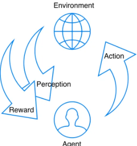
of view, it is more meaningful for us than other machine learning algorithms. Because reinforcement learning is like life. In most cases, we do not know what to do, so we have to try different approaches, in order to find a good choice. Meanwhile, life keeps changing, and we have to keep updating perceived knowledge. In 1.1, it shows the procedure of reinforcement learning. After the agent gets perception from environment, it makes an action based on its judgement, after that the environment returns a reward, facilitating the agent to make future actions.
Figure 1.1:Learning from Interaction
1.1
Exploration and Exploitation Trade-off
Exploration and Exploitation is first introduced by March [1991]. In that paper, March defined that exploration as "includes things captured by terms such as search, variation, risk taking, experimentation, play, flexibility, discovery, innovation" and exploitation as "includes such things as refinement, choice, production, efficiency, selection, implemen-tation, execution". In Levinthal and March [1993], the definition is more understandable: "exploitation is the use and development of things already known and exploration is the pursuit for new knowledge". The basic dilemma between exploration and exploitation is, exploration is taking the risk of uncertain payoff for a long-term goal, while exploitation is
taking sub-optimal action by the support of certain benefit. So the decision maker has to balance this trade off, maximizing the final goal.
The scenario we described above of searching good Wi-Fi signal is a typical scenario of exploration and exploitation. Since you need to explore which direction might give you better signal, but also try to exploit the place with the good signal. In reinforcement learning field, multi-armed bandit (MAB) problem is used as a classical example to model this kind of trade-off, making decisions sequentially by learning under uncertainty.
1.2
Bandit Problems
MAB problem was first introduced by Robbins [1952] in 1950s. In that seminal work, Robbins tackles the problem of sequential design for solving statistical problems that the sample data does not have fixed size and composition, deriving from observations. The term "bandit" comes from gambling slot machine. In a casino, there are some traditional slot machines, each one is with one arm. When pulled, each arm yields a reward drawn from a specific reward distribution of that arm. In the beginning, the gambler has no idea about all the machines and all the reward distributions. But after many times’ trials, he can focus on pulling those machines yielding better rewards. So the goal of this gambler is to maximize the total collected rewards.
1.2.1 MAB framework
According to different rewards distribution settings, there are different branches of MAB. Here, we only talk about stochastic and adversarial settings of MAB problem. To simplify the problem, the rewards are usually bounded in[0, 1].
In the Stochastic model, we assume that the rewards of each arm is an i.i.d sequence of random variables, which means each time the gambler pulls a certain arm, it randomly
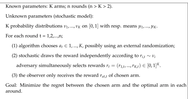
Known parameters: K arms; n rounds (n > K > 2). Unknown parameters (stochastic model):
K probability distributionsν1, ...,νK on[0, 1]with resp. meansµ1, ...,µK. For each round t = 1,2,...,n;
(1) algorithm choosesat ∈1, ...,K, possibly using an external randomization; (2) stochastic draws the reward independently according tori,t ∼νi
adversary simultaneously selects rewardsrt= (r1,t, ...,rK,t)∈[0, 1]K. (3) the observer only receives the rewardrat,t of chosen arm.
Goal: Minimize the regret between the chosen arm and the optimal arm in each around.
Figure 1.2:The framework of MAB in stochastic and adversarial rewards.
generates the reward associated to a stationary distribution. So rewards from the same arm in different trials are independent; also, rewards from different arms are independent. TheAdversarial model, however, has no restriction on the sequence of rewards, which means there is no statistical assumption when generating the rewards. For example, we can assume that for each machine, a mechanism sets the reward to some manually chosen values between 0 and 1. If this mechanism does not consider the gambler’s actions, we call it obliviously adversarial. Otherwise we call it non-obliviously adversarial.
We define the framework of stochastic and adversarial MAB problem in Figure 1.2. Both the stochastic model and the adversarial model are well studied in the MAB literature. The stochastic bandit model was first analyzed in Lai and Robbins [1985], which proposed the algorithm of upper confidence bounds for asymptotic regret analysis. And in Auer et al. [2002a], the authors systematically analyzed the adversarial bandit model, and proposed Exp algorithm family to solve this problem.
1.2.2 Contextual Bandit
Bandits problems exist in many places in real life, such as website optimization. Here is a simple example. A website designer wants to display one ad out of three on a page, but he does not know which one is better. In this scenario, the designer needs to find the best choice, but also during the testing time, he wants to have highest possible CTR1in order to gain more revenue. He plans to implement MAB algorithms to solve this problem, because it is an exploration and exploitation trade-off. After a while, he finds that ad A has the best payoff rate. More people are clicking ad A. But later he tasks himself, seeing as people have different taste, and he realizes that he does not need to display the same ad to everyone. With the user information this website collects, also called context, such as IP address. He finds that actually visitors from Asia click more on ad A, visitors from Africa click more on ad B and visitors from America click more on ad C. Because of the massive population of Asia, of course, he concludes more users click ad A. But if we can serve Asian visitors with ad A, African visitors with ad B, and American visitors with ad C, the website would have a higher revenue. When the bandit problem comes with context, it turns into the contextual bandit problem.
Contextual bandit can help you notice this kind of difference, and it is obvious that if you can serve ads to users in a more personal way, the revenue could be increased. Another example is about news article recommendation system. We discuss more details about it in the following chapters. But the idea is similar, by using contextual bandit algorithms to recommend the news to visitors, we consider about their user information to help us conduct personalized recommendation, contributing to the CTR increment.
Till here, we need to stress that the original motivation of this project is to research on bandit algorithms, especially contextual bandit algorithms, and evaluate if it is useful to be implemented in Softonic news article recommendation system. Unfortunately, during this 1Click-through rate (CTR) is a way of measuring the success of placing an online content by the number of
project we do not have sufficient data from Softonic or testing environment for experiments. So we build our own framework for testing and conduct our experiments with synthetic data and Yahoo! R6b dataset. All works are done in Python and R.
1.3
Contributions
Although the original motivation is about contextual bandit algorithms. But actually this thesis project does an overview of bandit algorithms in both context-free and contextual environment. It is very important to know more about context-free bandit algorithms, not only because it helps us understand some basic characteristics of bandit algorithms, but also because nearly all the contextual bandit algorithms are derived from context-free ones. This paper is conducted in a fairly practical way. Instead of focusing on mathematical proof, we put more effort on testing and comparing different bandit algorithms on both synthetic data and real product data. This thesis is the first work to discover context-free and contextual bandit algorithms together, and use synthetic contextual data as testbed to get more insight of bandit problems. We also test different algorithms on contextual bandit dataset. Finally, we summarize an executable way to solve problems like recommending news article to website visitors.
1.4
Road Map
The remainder of this paper is organized as follows.
In Chapter 2, we present the problem setting and definitions. Our objective is to use contextual bandit algorithm to solve personalized news recommendation with items of high churning attributes. So we present a contextual bandit problem setting, but can be easily simplified as context-free problem setting if we do not consider the context. The most import definitions are the same for each algorithm, such as CTR, selection strategy, update
policy, etc.
In Chapter 3, we present different bandit algorithms, including context-free and contextual methods. Epsilon-greedy, Softmax and UCB1 are the most popular algorithms in stochastic MAB, and regarding the adversarial model, Exp3 has a better theoretical weak regret bound, proved by previous work. In contextual bandit approach, we present LinUCB and LinearBayes, mainly because of the computation complexity is linear. These two algorithms are quite efficient in the real implementation. Also, we explain the idea of EXP4.P algorithm, comparing with LinUCB and LinearBayes.
In Chapter 4, we test these algorithms in synthetic datasets, including simple context-free synthetic dataset and contextual synthetic dataset. First, we want to observe the basic characteristics of context-free bandit algorithms. Then, based on what we have observed, we can further test them in the environment with context.
In Chapter 5, we test context-free and contextual bandit algorithms on Yahoo! R6b dataset, and compare the result in between. And we notice that contextual bandit algorithms, such as LinUCB, help us get a good result.
In Chapter 6, based on Yahoo! R6b data set, we have a surprising discovery that the very simple Clickrate policy outperforms LinUCB. After we analyse the data source, we define our own approach for this certain dataset, and extend this idea to a general approach of solving similar problems.
In Chapter 7, we review the development of bandit problems and algorithms over time. Literature review is to see bandits problem in a higher level after going into details of this project.
In Chapter 8, we conclude the studies and experiments. The drawbacks of this project and future works are presented.
Chapter 2
Problem setting and definitions
2.1
Introduction
In this chapter, we define the setting of multi-armed contextual bandit problem. Generally, this model can be used for online recommendation, such as news/ads recommendation on a website. As chapter 1 explains, bandit algorithms are good for this kind of exploration and exploitation trade-off, especially with high churning data. We saw the framework of MAB in the previous chapter. The basic difference between MAB and contextual bandit problem is if the bandit algorithm observes context or not. So here we just discuss the more complex setting, multi-armed contextual bandit problem.
2.2
Problem Statement
Nowadays, many websites are still using the traditional way, in which some pieces of news are chosen by editors, to recommend news to visitors every day. However, it is obvious that this is not a good approach. No matter how experienced the editors are, the decision of this recommendation is fairly subjective. There are some main issues in this approach.
Normally, editors select the news having biggest potential to get clicked by viewers. But, if, in fact, the news does not cater to users’ interests, it is very hard to detect without waiting a period to measure the CTR. Also, people have preferences of reading news. For example, a programmer may be more interested in clicking technology-related news, rather than a gossip news, which is more popular among teenage girls. So it could be more accurate if we introduce the personalization into news recommendation.
To solve these issues, we can model it as a multi-armed contextual bandit problem. Referenc-ing to the notation of Li et al. [2010] (with some variations), a contextual-bandit algorithm
Hproceeds in discrete trials t = 1,2,3, ... T. So that in trial t:
1. The algorithm observes a set A(t) of arms (e.g., in this thesis, we are talking about news) and the current userut with a feature vector xt (i.e., the context). Associated with each arm a is a payoffrt,a ∈ [0, 1]. rt,a, whose expectation decided by both userut and armat.
2. According to payoffs gathered in previous trials and the current user features, H
chooses an arm at ∈ A(t), and receives payoffrt,a. And we have to emphasize that there is no payoff value observed for armsa6=at.
3. Then the algorithm updates and improves its strategy of selecting arms with the new observation(xt,at,rt,at), including context, arm and reward.
Following the rules set up above, the algorithm wants to maximize the cumulative payoff in the long term. We define the total payoff after t trials as∑Tt=1rt,at. Normally, in bandit
problems, we are using the minimization of the regret between our policy with optimal policy which can always select the best arm a∗ at trial t, a∗(t). Similarly, the total payoff of the optimal policy is ∑Tt=1rt,a∗
t. So the T trial regret RH(T)for algorithm H is defined
formally by RH(T)==def E[ T
∑
t=1 rt,a∗ t]−E[ T∑
t=1 rt,at]. (2.1)If we set thext andAt the same for all t, we simplify this multi-armed contextual bandit problem into classical K-armed bandit problem, also called context-free bandit problem.
2.3
Discussion
Considering recommendation system, it is more often we hear about collaborative filtering and content based. But we choose bandit algorithms to solve this news article recommenda-tion problem instead of them. The biggest difference is classical recommendarecommenda-tion system needs a big amount of data in order to have an accurate prediction, but here, the data we are dealing with is coming dynamically with quite different features. In this situation, we need to catch the trend very fast, in a limited time, otherwise the news will become outdated and worthless. This is also a main difference between learning under certainty and learning under uncertainty.
In our scenario of this news recommendation system, at each time t, we can treat the pool of news asAt. Each news from the pool is an arm a, and the selected news isat at time t. We can observe that whether the user clicks that recommended news or not, so the payoff is 1 if the user clicks; otherwise the payoff is 0. It is obvious that the result is the common effect of both user interest and news content.
The goal of bandit algorithms is trying to maximize the total payoff, but for better evaluation, we always take the measure of minimizing the regret instead. In Equation (2.1), the framework is calculating strong regret bound of algorithms. It means we sum the payoff difference of optimal arm and selected arm for each trial. But some other algorithms use weak regret bound, such as Exp3. Instead of summing up the regret for each trial, we only calculate the regret of total payoff of selected arms, compared to optimal arm in terms of total payoff too.
Generally, bandit algorithms have two objectives:a) exploit the optimal arm to gain more payoff; andb) explore the non-optimal arms to increase the knowledge. These two objectives
together contribute to the final goal: maximize the cumulative reward in a long term. There are some parts we need to take into account in a real case. For example, feature construction is very important. Not only do you need to deal with the different data type of features, such as nominal, categorical, linear, etc., but also to reduce the dimensionality in order to control the data noise and the computation complexity. Moreover, normally, we assume that the K arms are fixed in our experiments. But in the real world, arms are constantly changing. If we do not set proper starting strategy for those new arms, the results may be influenced greatly by this kind of "cold start".
Chapter 3
Bandit Algorithms
3.1
Introduction
In this chapter, we briefly present the most widely used context-free bandit algorithms. Apart from their Pseudo-codes, we discuss the theoretical characteristics of these algorithms. The first three algorithms aree-greedy, Softmax and UCB1. They address stochastic setting
problems more effectively compared with adversarial setting, see Bubeck and Cesa-Bianchi [2012]. Then we introduce Exp3, which is a strong candidate in the adversarial model. Finally, we explain three algorithms considering contexts, LinUCB, LinearBayes, and Exp4P. However, we only choose the implementation of LinUCB and LinearBayes in this thesis project. The reason for not choosing Exp4.P is presented in the following sections.
According to problem setting and definitions, algorithms select arm according to the knowledge they perceived and the policies they defined. Different arms have different probabilities to get clicked. To measure the accuracy, we have different criterion, such as the probability to select the optimal arm, or cumulative payoff/CTR, and so on.
3.2
e
-greedy
e-greedy is one of the simplest algorithms in context-free group. From its literal meaning,
we can understand that a greedy algorithm always selects the option bringing the largest payoff at that point. However, if it is only a greedy algorithm, then there is no exploration, but exploitation. Watkins [1989] first described e-greedy algorithm to solve
exploration-exploitation problem. The idea is in each trial, with probability of 1 - e, the e-greedy
algorithm exploits the best payoff arm, and with probability ofe, the algorithm randomly
uniformly explores all the arms in order to gather more information for a reliable decision. As you can see in Figure 3.1, for each step ofe-greedy algorithm, it follows this process.
Figure 3.1:e-greedy Arm Selection Process
There is also a slightly changed version of thee-greedy algorithm, in which isedecreases by
time, also called annealinge-greedy. The reason we can changeevalue over time is because
it is not necessary to keep the same exploration if we gain more and more knowledge to ensure the right action. A simple example: there are only two arms, A and B, holding payoff rate of 0.1 and 0.9 separately. With the possibility ofe, they always have the same chance
to get selected. But if eis decreasing, we can get more payoff each time, since we could
exploit more the arm with payoff rate of 0.9. However, the performance depends on the reward distribution of each arm greatly. However, in Vermorel and Mohri [2005], based on
an empirical experiment, the authors did not find the support that annealinge-greedy has a
good practical performance. We will not test it in the experiment session.
3.3
Softmax
Softmax, also one of the probability matching methods, is selecting the arm based on its probability proportion of the estimated values. This idea was first introduced by Luce [1959]. Arms with higher recorded rewards have a higher possibility to get selected. Unlike
e-greedy the algorithm does not know the difference between all the arms when it needs to
explore them. Softmax offers a more structured exploration by selecting arms in proportion to their estimated values. It uses exponential expression to turn any negative value into positive, ensuring the probabilities do not have strange values. Imagine if we only have two arms, then the probabilities of getting selected are computed as follows:
P(A) = e rA/tau erA/tau+erB/tau (3.1) P(B) = e rB/tau erA/tau+erB/tau (3.2)
Softmax is also called Boltzmann Exploration, because it uses Boltzmann distribution to select the arm each time. Boltzmann distribution controls how random Softmax is. There is a temperature variable in it. Just like what happens in chemical experiments, the molecules move faster when the temperature is high; otherwise they are more stable. If we set the temperature variable as zero, then we will always choose the arm with highest estimated value; if we set the temperature variable as infinite, the arm selection strategy would become purely random. So it is very important to tune the temperature value in order to get good results in experiments. Similar to annealinge-greedy, there is also annealing Softmax
algorithm. At first, the temperature variable is larger in order to ensure enough exploration, but by time, it decreases to get higher probability choosing the optimal arm to exploit more. However, according to Vermorel and Mohri [2005], still annealing Softmax algorithm does
not have a very good performance in the empirical experiment. We will not test it in the experiment session.
Algorithm 1Softmax Algorithm
Parameters: Realtau(temperature of Boltzmann distribution)
Initialization: ri(1) =1 for i = 1,...,K (ri is the click rate for each arm).
1: fort =1, 2, ...do 2: pk(t)← e rk tau ∑n i=1e ri tau
3: Drawit randomly according to the possibilities p1(t), ..., pK(t)
4: Receive reward xt 5: end for 6: for j=1, ...,Kdo 7: Updateri(t+1) 8: end for
3.4
UCB1
Frome-greedy and Softmax algorithms, we can see that they do not keep tracking that
how little they know about each arm. The estimated value we got is with noise. The more we explore them, the more confidence we will get to be sure about their payoffs. UCB algorithm can combine the degree we know each arm, here also called confidence, with estimated values when selecting arms. There are many members inUCBalgorithm family. UCB1 is the most basic one. It can be summarized by the principle of optimism in the face of uncertainty. It is like, although we lack sufficient knowledge about all actions, we hold an optimistic inference of how much reward we can get from each arm and select the arm with the highest inferred reward. If the inference is accurate, we would have a higher chance to exploit that arm again and receive less regret. Otherwise, the inferred reward will drop off fast, and we will explore other options. This inferred reward, we call it upper confidence bound, hence the acronym UCB.
Unlikee-greedy and Softmax, UCB1 has no randomness, to some degree, reducing the
stores the number of arms being selected asni. So at each timet, the algorithm picks the arm j(t)as follows: j(t) =arg max i=1...k (µˆi+ s 2 lnt ni ) (3.3)
3.5
Exp3
Till now, we have already seen the algorithms which are more suitable for bandit problems of stochastic setting, where each arm has a reliable probability to get clicked. So the task is to find the optimal arm as soon as possible and then exploit it. Thinking over the previous three algorithms,e-greedy and Softmax are more gullible. They might be misled by some
unstable rewards. UCB1 is optimistic in the face of uncertainty, by assessing our knowledge about all the arms.
In real world, there are more complex payoff structures. When the payoffs become com-petitively mannered, such as stock trading, being optimistic seems too naive. In this kind of adversarial setting, Exp3 is expected to be better in selecting arms. Exp3 is short for Exponential-weight algorithm for Exploration and Exploitation. This algorithm keeps a list of weights for each arm, and mainly selects arms uniformly according to their weights at each round. If the choice is good, the weight of that arm will increase, otherwise, it decreases. Also, we have the factorγto tune the algorithm, seen in Algorithm 2, deciding
to which degree to select arms uniformly.
The reason we think Exp3 is more suitable for adversarial bandit setting is because, even it finds a good arm to pull, still it keeps an eye to those arms with bad performances. The world may turn everything upside down immediately. Exp3 is more cautious to changeable payoff distributions of arms.
Algorithm 2Exp3
Parameters: Realγ∈ (0, 1]
Initialization: wi(1) =1 for i = 1,...,K (wi is the weight for each arm).
1: fort =1, 2, ...do 2: pi(t)←(1−γ) wi(t) ∑K j=1wj(t) + γ K
3: Drawit randomly according to the possibilities p1(t), ..., pK(t)
4: Receive reward xt 5: end for 6: 7: for j=1, ...,Kdo 8: ˆ xj(t) = ( x j(t) pj(t) if j= it 0 otherwise, 9: wj(t+1) =wj(t)exp(γxˆj(t)/K) 10: end for
3.6
LinUCB
LinUCB, first introduced by Li et al. [2010], is derived from UCB. Like its family members, it also contains 2 parts: estimated payoff and uncertainty term. Given the contextxt,a of each trial, LinUCB assumes that the expected payoffrt,a of each arm is linear in the current feature vector with an unknown coefficient vectorθ∗a,
E[rt,a|xt,a] =xTt,aθa∗. (3.4) From Walsh et al. [2009], it demonstrates the confidence bound for expected payoff for each arm, with probability at least 1−δ,
x T t,aθˆa−E[rt,a|xt,a] ≤(1+ q ln(2/δ)/2) q xTt,a(DTaDa+Id)−1xt,a. (3.5) Based on this inequality, LinUCB algorithm is defined in the following pseudo-code.
Algorithm 3LinUCB
Parameters: Realα∈R∗
1: fort =1, 2, ...do
2: Observe features for each trial: xt,a ∈Rd
3: for each arm a∈At do
4: ifa is not newthen
5: Aa ←Id 6: ba ←0d×1 7: end if 8: θˆa ←A−a1ba 9: pt,a ←θˆTaxt,a+α q xTt,aA−a1xt,a 10: end for
11: Draw armat =arg maxa∈At pt,a, and receive corresponding payoffrt 12: Aat ←Aat+xt,atxTt,at
13: bat ←bat+rtxt,at 14: end for
Like all UCB algorithms, LinUCB chooses the arm with highest upper confidence bound. This algorithm has some advantages. First, its computational complexity is not high, since it is linear in the number of arms and, in the worst case, cubic in the number of features. There are some other ways to reduce the complexity, such as feature engineering or updating the weights periodically. Second, this algorithm has a good scalability of dynamic arms. This is quite useful, since in the real recommendation system, normally the content pool is always changing.
3.7
LinearBayes
Linear Bayes derives from a simple idea. User’s preference of each arm is decided by certain features. For example, if an arm is always pulled by users holding some certain features, when a new user with similar features arrives, it is very likely that the algorithm would recommend the same arm. However, the probability of selecting an arm should also rely on the importance of features. For example, a feature occurs all the time, it seems important for each arm if we see them separately. But, of course, it is not true. If we only simply sum up all the individual features, we do not give sufficient weight to those more important ones. In Martín H and Vargas [2013], the authors describe the procedure of coming up with this bandit algorithm.
We usePa,i(t), Pa(t), and Pi(t)to represent the CTR of arm on each feature, of each arm, and of each feature itself. As it shows above, we use CTR of each arm and each feature to adjustPa,i(t), the selection strategy could be displayed as:
a(t) =arg max(
∑
i6=0 Pa,i(t) Pa(t) Pi(t) ). (3.6)We can see from this equation,Pa,i(t)is multiplied by inverse of overall click rate of feature i and Pa(t). The functionality of Pa(t) is to increase the chance of popular arm getting selected. The functionality ofPi(t) is more of balancing the weight of all features. For a certain feature, if an arm has a high CTR of it, but the feature itself has a low CTR, we can assume that this feature is highly relevant to this arm. Oppositely, when an arm has a low CTR of that certain feature, but the feature itself has a high CTR, meaning this feature nearly has nothing to do with this arm. When we go deeper of the definitions of parameters, we can get these following equivalences:
P(xi |a)≈ Pa,i(t) (3.7)
P(xi)≈ Pi(t) (3.8)
According to this, Eq.(3.4) is equivalent to: a(t) =arg max(
∑
i6=0 P(a)P(xi(t)|a) P(xi(t)) ). (3.10) a(t) =arg max(P(a| ∪xi(t))). (3.11) So the arm selection strategy is a linear approximation to the Bayes’ rule, the probability of selecting arms by given current context.3.8
EXP4.P
Exp4.P is a modification of Exp4 algorithm of Auer et al. [2002a]. It increases the guarantees for getting a good regret bound compared to Exp4. So Exp4.P stands for Exponential-weight algorithm for Exploration and Exploitation using Expert advice with a high Probability. But the basic idea is the same as Exp4 algorithm. Different from Exp3, which keeps tracking the weight of each arm, in Exp4, algorithm is tracking the weight of each policy, referenced to the experts. Each expert offers a policy to map the context to different arms. These policies are generated by supervised learning. In Beygelzimer et al. [2010], the paper shows how to use Exp4.P to obtain, in d VC-dimension, regret bound asO(√KTlnN).
But, like its predecessors, Exp4.P has an apparent drawback that it has to keep the weights over experts. That is the main reason we do not choose it to implement. When N is too large, the computational workload is massive. In that sense, Exp4.P will not be efficient. Beygelzimer et al. [2010] tries to relief this issue, so they cluster all the users instead of keeping the original features. But, even though, with six user clusters and 20 arms, the number of policies is 206, which is not small at all.
Compared to LinUCB and LinearBayes, Exp4.P needs to process data with supervised learning algorithms first to form appropriate policies, otherwise the algorithm may not be able to generate reliable arm selection strategy. What is more, because of the combination of
adjusted weights and uniform distribution, it makes Exp4.P more appealing in adversarial model of bandit problem. As we mentioned before, the computation is too heavy for our machine, we will not implement this algorithm in the experiment section. However, it could be a strong candidate for solving bandit problems with a strong computation capability.
Chapter 4
Simulations
4.1
Introduction
In this chapter, we conduct experiments in two different types of simulation datasets, context-free synthetic data, and contextual synthetic data. In both types, we create varied bandit problems to help us understand bandit algorithms better in different settings and to form our own approach of solving the contextual bandit problem in real world.
4.2
Experiments with context-free synthetic data
Settings: Number of arms, K is 5. Each arm generates payoff 1 according to Bernoulli
distribution with possibilities 0.1, 0.1 ,0.1, 0.1 and 0.9. It means, at each trial, the algorithm needs to select one arm out of five. And each arm has an individual and fixed probability to get clicked. If the arm generates payoff 1, meaning that this arm is clicked once. The goal is to maximize the total payoff, which is also equal to select the optimal arm as frequently as possible.
(a)With the initial value as 1 (b)With the initial value as 0
Figure 4.1:Difference of initial values
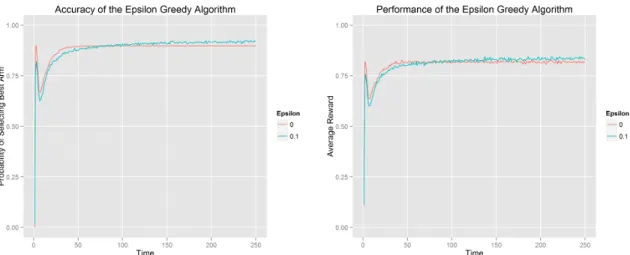
with the initial value as 0 and 1. Both graphs in Figure 4.1 present the average reward over time. The number is calculated by the average amount of total clicked number. We can see that 4.1a always performs better than 4.1b. It means that with the initial value as 1,e-greedy
algorithm can find the best arm faster. Besides, another thing that interests us is that it seems the smaller the epsilon value is, the higher average reward it can get. So we make another experiment to see the influence of different epsilon values.
In Figure 4.2, we compare the result of epsilon as 0.0 with as 0.1 in probability of selecting best arm and average reward. To our surprise, they almost have the same behaviors in both comparisons, probability of selecting best arm and average reward. It shows that it might not be necessary to spend time exploring arms. However, after analyzing, we conclude when we set the initial click rate of each arm as 1, it has already guaranteed a stage of exploration in a reasonable way. And the reason that exploration seems does not work is mainly because all arms here have fixed and stable payoff distribution and the reward difference is notable, it is easy to detect the optimal arm and exploit it. In this case, even pure greedy algorithm could perform quite well.
(a)Difference in arm selection (b)Difference in average reward
Figure 4.2:Different epsilon values
Similarly, we run Softmax on the same synthetic dataset. We can see from Figure 4.3, that the lower temperature gives us a better result. As we explained in Chapter 3, temperature variable is used to control the degree of randomness of selecting arms, here the arms’ reward distributions are stable, so we do not need a high temperature value to explore too much.
(a)Average reward (b)Cumulative reward
Figure 4.3:Softmax with different temperatures
Now, we have already implemented epsilon-greedy and Softmax algorithms, and found that in this setting environment, both algorithms should take more aggressive strategies. So we choose 0.1 as both epsilon value and temperature value, comparing with UCB1 algorithm
(a)Average accuracy (b)Cumulative reward
Figure 4.4:Comparisons of epsilon-greedy, softmax and UCB1 in 250 trials
(a)Average accuracy (b)Cumulative reward
Figure 4.5:Comparisons of epsilon-greedy, softmax and UCB1 in 1000 trials
in the same testbed. The first thing catches our eyes is the noise of UCB1, compared to the other two, UCB1 seems not stable at all, although it is the fastest algorithm finding best arm. The reason of its backpedaling is that upper bound confidence value contains an uncertainty part, to measure how little we know about each arm, in order to pay more attention to those unknown arms.The impact of backpedaling keeps decreasing by time, but never disappears. From Figure 4.4b, we can see in terms of cumulative reward, and Softmax performs best and UCB1 performs worst. While from Figure 4.4a, UCB1 starts to catch up with Softmax since 100th trial. We tried another test, setting total trials number up to 1000. We can see in Figure 4.5, UCB1 outperforms epsilon-greedy and gets very close to Softmax. It demonstrates great potential regardless of those continuous dips.
After we saw three popular algorithms in stochastic setting, we would like to bring Exp3 into the discussion. It has a sound weak regret bound. The idea is instead of comparing selected arm with the optimal arm in each single trail, we only compare the difference between the highest cumulative reward generated by one single arm and real cumulative reward summed by all selected arms. In Figure 4.6, we only compared Exp3 with UCB1, within our expectation, Exp3 with less gamma value has better performance in terms of cumulative regret, but takes more time to discover optimal arm. But clearly, Exp3 performs worse than UCB1.
(a)Average accuracy (b)Cumulative reward
Figure 4.6:Comparisons of UCB1 and Exp3
In order to see the performances of these four algorithms varying in different setting, we did more experiments with changed K value and reward distribution. Similar to the setting above, K is the number of arms, and each arm has its own reward distribution. This distribution decides the probability of each arm getting clicked. But here the payoff is not as stable as what we saw above, there are different variance on expectations. The goal is also to find which algorithm can collect the highest cumulative payoff.
Setting: Number of arms, K∈ [2, 5, 10, 50], the mean reward expectations of all arms are generated between[0, 1]by random function based on Gaussian distribution. Each arm has variance of 0.01, 0.1 or 0.5. We run each test 100 times with 1000 trials and calculate the average value for each algorithm.
(a)Cumulative reward with K=10, Var=0.01 (b)Cumulative reward with K=10, Var=0.1
(c)Cumulative reward with K=10, Var=0.5 (d)Cumulative reward with K=50, Var=0.01
(e)Cumulative reward with K=50, Var=0.1 (f)Cumulative reward with K=10, Var=0.5
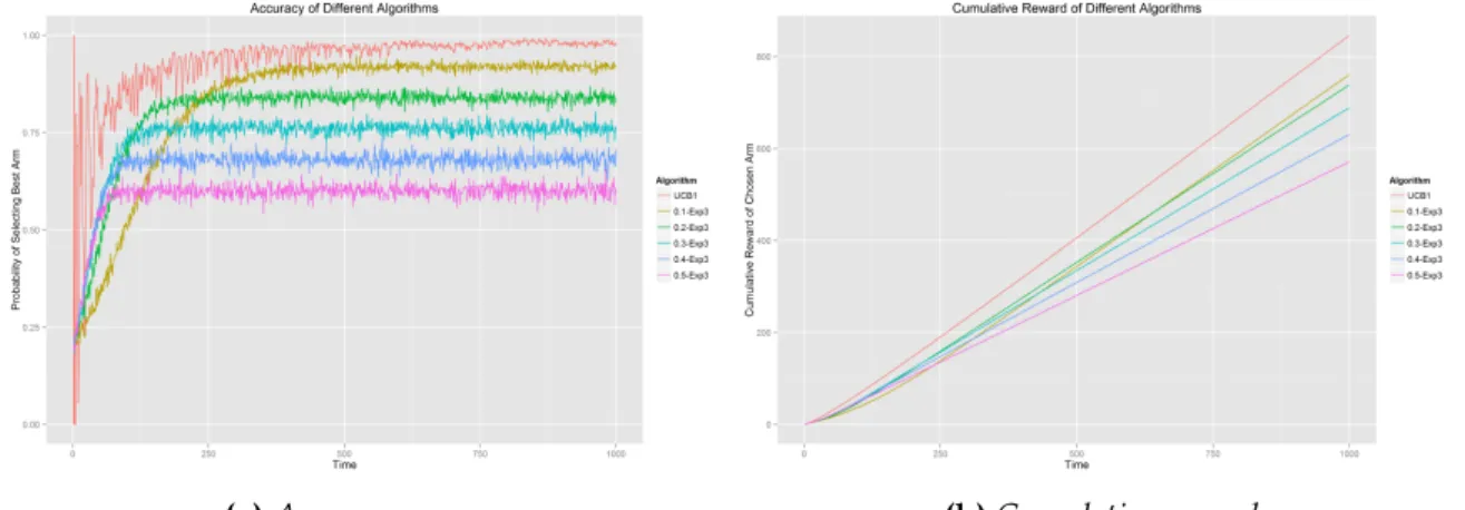
Observation: From Figure 4.7, we can see that the simplest algorithm, e-greedy always
performs very well. Softmax has a very good performance too, although it is slightly worse thane-greedy. Both of them are heuristics algorithms.
A very striking observation is that in K=2 and Variance=0.1, 0.5, shown in Figure 4.8a and Figure 4.8b, Exp3 outperforms Softmax and UCB1. Normally, in empirical experiments, it is very hard to find a setting that Exp3 can beat UCB1, even in the adversarial environment. In this case, we get a hint that Exp3 could be considered as a good option when K is small.
(a)Cumulative reward with K=2, Var=0.1 (b)Cumulative reward with K=2, Var=0.5
Figure 4.8:Bandit problem setting where Exp3 wins
Besides, for each algorithm, the performance is influenced greatly by the characteristics of arms. When K is small, all algorithms have similar results, such as Figure 4.8a. They have slight difference, but it is not that obvious. When K is large, for example equal to 50, the difference of cumulative rewards is very large. In Figure 4.9, both e-greedy and
Softmax outperform the other two rivals by almost 50% in cumulative payoff. Meanwhile, thee-greedy in much precise in terms of selecting the optimal arm.
UCB1 has a better performance when K is small, but it cannot catch the variance of arm very well. The coverage of UCB1 is also slower than other algorithms, due to its balance of exploration considering how little we know each arm. From Kuleshov and Precup [2014], it shows that UCB1-Tuned perform much better with arms with larger variance.
(a)Average accuracy with K=50, Var=0.01 (b)Cumulative reward with K=50, Var=0.01
Figure 4.9:Experiment results with K=50, Var=0.01
Sometimes even Softmax can have a good result, but it could not find the optimal arm. In the comparisons of Figure 4.9, the graph of average accuracy shows that Softmax has nearly the same accuracy to select optimal arm as UCB1 and Exp3, but it has the total payoff similar toe-greedy, which demonstrates that even it did not find the best arm, but it still
can track the sub-optimal arm, ensuring the result. Exp3 is proved to have a robust bound in adversarial environment, so we did not expect Exp3 yielding a good result here.
Apart from the experiments above, we conduct other experiments of adversarial bandit setting. Opposite to stochastic one, where all arms have i.i.d reward distribution. We do not have any condition on arm behavior. It is possible that some good arms can turn into super bad suddenly. Similarly, we evaluate performances of the algorithms by tracking their CTR and ability of selecting optimal arm.
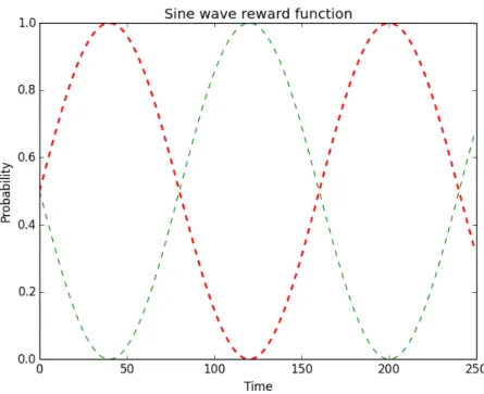
Setting:Number of arms, K is 2. Each arm generates payoff 1 according to Bernoulli distri-bution of sine wave reward function. The probability follows this formula, A(sin(ωπt/10+ ϕπ) +d). To control the bound of generated reward, we set A as 0.5 and d as 1, so that this
sine wave function will generate the probability of reward∈ [0, 1]according to time t. Arm 1 and 2 have [[0.125, 0],[0.125, 1]]as(ω,ϕ)separately. Shown from Figure 4.10, Arm 1 and
Arm 2 have symmetric behaviors and both are changing all the time. We also set gamma value as 0.1 in Exp3 algorithm.
Figure 4.10:Sine wave reward function
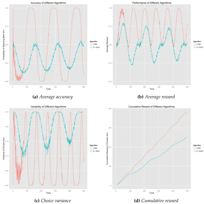
Observation:In this setting of two symmetric arms, we just set the best arms as Arm 1, and the accuracy of selecting optimal should change from 0 to 1 periodically. To our surprise, UCB1 can catch this change precisely. From Figure 4.11a, we can see the performance of UCB1 meets our expectation ideally, but Exp3 cannot perceive this kind of change in time. In Figure 4.11b, the average reward of UCB1 is also always above 0.5 and finally it generates a cumulative reward around 400 out of 500 trials. From our observations of these context-free experiments, we can see that UCB1 is quite strong in both stochastic and adversarial settings. And although Exp3 has a good weak regret bound from the mathematical demonstration, but it does not ensure a good result in the practical dataset. Most probably, our synthetic dataset does not suit the requirements of Exp3.
(a)Average accuracy (b)Average reward
(c)Choice variance (d)Cumulative reward
After talking with Prof. Peter Auer, he pointed out that this sine function is not a good testbed for either EXP3 or UCB1, since it is time variant. Both algorithms are not sensitive for time-varying rewards. Later he suggested that there is a simple setting where Exp3 can beat UCB1 if and only if when T is rather large:
arm1(t)= 1/2, for allt
arm2(t)= 1/4, fort =1, ...,T/4 arm2(t)= 3/4, fort =T/4+1, ...,T
(a)Average accuracy (b)Cumulative reward
Figure 4.12: Comparisons of UCB1 and Exp3 in adversarial setting from Peter Auer
We tested with T equals to 100000, seen from Figure 4.12. Even with T equals to 100000 is not large enough to see the expected result. The cumulative rewards are very close, but still UCB1 is slightly better than Exp3. We assume that if we set T much larger, we can see that Exp3 beats UCB1. From these observations, we can only conclude that in some cases of adversarial setting, Exp3 might have a good performance. Nevertheless, it could not guarantee the consequences, especially when data generation process is unknown. Because it is a worst case result, making it overly pessimistic about the world. While, UCB1 is quite optimistic. But neither of them can track fast-changing arms, what they try to do is finding the arm that performs best in the long term. Till now, we have an overview of context-free
algorithms and comparisons in different bandits problems. It is time to move to scenarios of problems with context.
4.3
Experiments with contextual synthetic data
In this section, we test algorithms on synthetic contextual data; the main goal is to check if context helps to improve CTR in this kind of recommendation. However, because of the limitation of dataset itself, it is hard to explain the results in theory, we record the performances and make some reasonable interpretations.
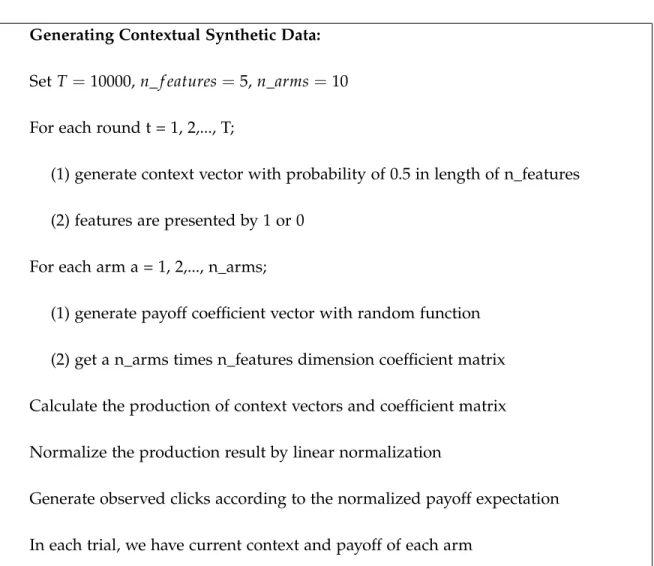
Settings:First of all, we want to stress that, unlike the problem definition in chapter 2, this synthetic contextual bandit dataset is a full-label problem. It means that we have the reward feedback of each arm instead of just the chosen arm. This original dataset contains 10000 records, each record is made up of context and rewards of all arms. We have 5 features in context and 10 arms in the selection pool. The payoff rate, in another word, the probability of arm to get clicked, is decided by LinUCB algorithm. Equation 3.4 explains that the expected payoff of each arm is a linear function of current features. The details of the process are presented in Figure 4.13.
Generating Contextual Synthetic Data:
SetT=10000,n_f eatures=5,n_arms=10 For each round t = 1, 2,..., T;
(1) generate context vector with probability of 0.5 in length of n_features (2) features are presented by 1 or 0
For each arm a = 1, 2,..., n_arms;
(1) generate payoff coefficient vector with random function (2) get a n_arms times n_features dimension coefficient matrix Calculate the production of context vectors and coefficient matrix Normalize the production result by linear normalization
Generate observed clicks according to the normalized payoff expectation In each trial, we have current context and payoff of each arm
Figure 4.13: The procedure of generating contextual synthetic data.
Observation:From this problem setting, the reward information of all the arms is presented, so we just need to simply compare the cumulative payoff of each algorithm. From Figure 4.14, we can see that although the difference of cumulative payoff of different algorithms is not that large, LinUCB has a better result than other context-free algorithms. But LinearBayes performs worst among all the candidates. For further observation, we test with varied values of T, n_arms, and n_features.
In Figure 4.15, we can see T equals to 100000, n_features equals 10, and n_arms equals to 20. Similarly to Figure 4.14, LinearBayes does not perform well and LinUCB performs the best. We also find that UCB1 has exactly the same cumulative payoff as LinUCB. After
Figure 4.14:Testing Results of {10000,5,10}
carefully checking the payoff of each trial, these two algorithms obviously have different arm selection path. To understand UCB1 and LinUCB better, we set up another experiment.
Figure 4.15: Testing Results of {100000,10,20}
In the third setting of synthetic contextual setting, we multiply both T and n_features by 10, and keep the same n_arms. With this setting, we can compare with Figure 4.15, how bandit algorithms behave when feature matrices are high dimensional. Within our expectation,
Figure 4.16:Testing Results of {1000000,100,20}
UCB family has a very reliable performance. Nevertheless, to our surprise LinearBayes nearly reaches the same accuracy as LinUCB. One possible explanation is that LinearBayes works better when feature number is large, or when trial number is large. According to Figure 4.16 and the other two tables above, we can conclude that:
1. Context helps, but it depends on the very case.
2. UCB algorithm family has stable performance in different settings.
3. The results of different algorithms could vary dramatically according to attributes numbers.
To explain why UCB1 outperforms LinUCB in Figure 4.16, we need to review the data generation process. Each feature has an equal probability to get selected for all visitors. At each round, based on the setting, several arms hold payoff as 1. These characteristics do not follow the rule of real world. We can also see that it is very hard to mimic user log data. Finally, we will test these algorithms on real product data from Yahoo! Labs. This dataset guarantees an unbiased evaluation emprirically.
Chapter 5
Unbiased Evaluation (Yahoo! R6b
dataset)
5.1
Introduction
The testing dataset we are using in this project is called Yahoo! R6b, from Yahoo! Webscope Program. It contains a fraction of traffic of user visits on the Yahoo! front page. It records the user click logs for news articles displayed in the Featured Tab of the Today Module. The recommended articles are selected uniformly at random. So that this dataset allows unbiased evaluation of bandit algorithms, presented by Li et al. [2011]. This dataset contains data collected from 15 days of October, 2011 (from October 2 to 16). There are about 30 million user visits during that period, and the dataset records features of users with dimension 136 in binary format. These features include personal information, geographical information, etc. But feature definitions are no revealed. For each record from this dataset, the following 5 sections are logged in order:
1. the timestampti of this visit, such as "1317513291"
3. the reward of this recommendation, either being clicked or not, presented by "1" or "0" 4. the presence of features of the present visitor, split by "|user", the index of observed
features, such as "1 9 11 13 23 16 18 17 19 15 43 14 39 30 66 50 27 104 20"
5. the article pool, which contains the ids of all articles, such as "|id-552077 |id-555224 555528 559744 559855 560290 560518 560620 563115 |id-563582 |id-563643 |id-563787 |id-563846 |id-563938 |id-564335 |id-564418 |id-564604 565364 565479 565515 565533 565561 565589 565648 |id-565747 |id-565822"
Here, to connect to problem definitions, we recall the environment of the bandit algorithm first.
1. The algorithm observes a set A(t) of arms (e.g., in this thesis, we are talking about news) and the current userut with a feature vector xt (i.e., the context). Associated with each arm a is a payoffrt,a ∈ [0, 1]. rt,a, whose expectation decided by both userut and armat.
2. According to payoffs gathered in the previous trials and the current user features,H
chooses an arm at ∈ A(t), and receives payoffrt,a. And we have to emphasize that there is no payoff value observed for armsa6=at.
3. Then the algorithm updates and improves its strategy of selecting arms with the new observation(xt,at,rt,at), including context, arm and reward.
We can see, with Yahoo! R6b dataset, the article pool is setA(t). Timestamp could stand for individual visitor, user feature, or even article feature. For example, we can use timestamp to record the appearance time of each article. And payoffrt,a is exactly the boolean value indicating whether this visitor clicked the recommended article or not. Finally, we also observe user features from logged file. To simplify the computation complexity, we transform
them into binary feature vectorsxt. Another thing we need to stress is that only if articleai recommended by algorithm matches the article id recorded by that instance, we evaluate it, updating our policy. This offline evaluation method is studied by Li et al. [2011]. The goal is to realize offline evaluation with logged data instead of a simulator, with the fact of nearly impossible to simulate user behaviors in this environment. This evaluation method ensure unbiasedness guarantees, by sacrificing data efficiency to some degree. Considering experiment time, we only test algorithms with the first one third of data.
5.2
Evaluation results
In order to check if bandit algorithms help, we run random arm selection policy first, as the bottom line. The idea is to randomly recommend articles to visitors, meaning no recommendation. From Figure 5.1, we can see that till 920,000 records, random arm selection can reach CTR a little bit below 0.037, very poor result.
Then we run other algorithms and compare them together in the same graph, Figure 5.2. From the very beginning,e-greedy arm selection policy wins random policy, and its CTR
increases rapidly in the first one third period. After that it becomes relatively flat. At last, it reaches CTR about 0.076.
Figure 5.2: Results
The result of Softmax is not stable. It has a good starting point, but then it goes down till record 3,000,000 before recovering. Finally, it ends with CTR around 0.050.
UCB1 has a much better performance. Its CTR increases very fast from the beginning and reaches above 0.055 at last.
Exp3 has a similar behavior with UCB1 policy. But the final CTR is only 0.046.
LinUCB has a good result. We can see it takes some time to train the algorithm in order to select suitable arms based on user features. Finally, it surpasses 0.08, making us believe that LinUCB is a very good option in solving contextual bandit problems.
LinearBayes has an unpredictable behavior from our previous experienc. And this time, obviously, it does not perform well. The result is even worse than random recommendation, which means it always selects bad arms.
Chapter 6
Tailored Solution
In chapter 5 and chapter 6, we have already seen how differently algorithms behave in different situations, such as stochastic, adversarial, context-free, contextual, etc. And contexual bandit algorithms do help in the datasets we tested. However, when we come to a real dataset, normally there is no way for us to figure out its real property ahead of time. Since in the real world, datasets are always quite complex, and often mixed with multiple characteristics. So in this chapter, we try to build our own approach suitable for Yahoo! R6b dataset. It might not be a general method for all bandit problems, but it offers another possibility to solve practical bandit problems. As we discussed before, we want to implement bandit algorithms to solve automatic content selection problem, and the goal is to increase CTR of news articles, so in evaluation graphs, we just use the CTR as performance index to judge the algorithms.
The simplest idea is that we can just recommend to all visitors the article with the largest click number. In the beginning, we have no clue which arm is better, so we randomly select arms to explore. From Figure 6.1, we can also see that the result is not so good.
The second idea is like epoch-greedy, in each epoch, we run e-greedy policy first, then
Figure 6.1:Result of Mostclick Policy
efficient. This approach is rejected even without testing, because the biggest drawback is that this approach separates exploration and exploitation completely. One period is for exploration, and the other period is for exploitation, keeping alternating. News article recommendation is to deal with high-churning data and we cannot control or notice the changes in advance. Just imagine, if the latest news is very popular, but at that time, we were in the exploitation stage, where we just exploit the best arm concluded from last epoch. We could miss the chance to get higher CTR from upcoming news because of the lagging of a notice behind its appearance.
The third idea is to recommend arms with highest CTR to visitors. It sounds risky. Because if we are not lucky at all, we might choose a bad arm and exploit a lot. However, according to our previous experiments. we can relieve this issue by setting initial CTR of all arms as 1. In this case, it already guarantees a complete exploration at the beginning. It does not matter if we are with luck or not, if we did not select a good arm, the algorithm will switch to another option. If the other options are worse, the algorithm will return to explore
the original arm again. This is quite an aggressive approach. To our surprise, it is a big success. It reaches 0.0877 in the end with a growing trend, seen from Figure 6.2. We wonder why Clickrate has such a good performance. Because when UCB1 policy selects the arm, it also contains click through rate in expected value, but the final result is much worse than simple greedy policy. One possible answer is that in this dataset, we do not need to use the uncertainty part to balance exploration and exploitation that much. Because the payoff rate is quite reliable. Extra exploration stage can only result in a potential loss of CTR.
Figure 6.2:Result of Clickrate Policy
As we said, from our observation, the uncertainty part is not that important. But we have two other assumptions that CTR is related with time and context. The impact of context is proved already. For proving the impact of time, we did a simple test. We compared two policies together, one is recommending the earliest news article in the content pool, and the other is recommending the latest news article in the content pool. The result is super clear that time matters, because there is a huge difference between Earliest policy and Latest policy.
Figure 6.3: Time impact
Finally, we combine the value of Clickrate, the context-influenced part of LinUCB, and the time impact factor, assigning proper weights to all of them. To tune weights, we were using grid search method, by defining possible component weights and testing all possible combinations between them. Finally, we found a good balance point between these three components. So our approach is mainly based on simple Clickrate policy, with consideration of context factor and time impact.
In Figure 6.4, we can see it outperforms Clickrate policy, but they almost have the same shape of CTR trend.
Chapter 7
Literature Review
The original study of bandit problems can be traced back to Thompson [1933], the problem was about clinic trials. There are different treatment approaches targeted to a certain disease, the doctor needs to decide which one to choose for the next patient. For sure, the doctor wants to treat as many patients as possible.
However, multi-armed bandit problems were first formalized by Robbins [1952]. This work was built on the achievements of Wald [1973] and Arrow et al. [1949], both of which focused on sequential decision making under the support of Bayes probabilities. In Robbins [1952], the stochastic bandit problem setting with set up. And it is further analyzed by Lai and Robbins [1985] with the i.i.d condition of arms with fixed reward distribution. They built a logarithmic lower bound algorithm to select sub-optimal arm by an optimal policy in each trial with limited times. In the same year, another work, Berry and Fristedt [1985], overviews bandit problems from the point of view of statistics, presenting multi-armed bandit with many variations.
In Whittle et al. [1981], the author researched multi-armed bandit problems with dynamic programming method, and he stressed the fundamental contribution of Gittins, especially Gittins and Jones [1974], Gittins [1977], Gittins [1979]. And in Gittins [1989], the second
edition of "Multi-armed Bandit Allocation Indices" describes Gittins’ original index solution to MAB problem and his following research work of different type of sequential resource allocations and stochastic scheduling problems. Gittins also refers clinic trials problem as the "chief practical motivation" for the design of bandit algorithms.
In context-free bandit problems research, from the beginning, the researchers mainly focused on the design of simple heuristic policies, like what Lai and Robbins did and achieved. Till 1995, Auer et al. [1995] introduced Exp3 and Exp4 algorithms, bringing MAB problems into adversarial setting. The biggest difference between Exp algorithms and previous heuristic algorithms is that Exp algorithms do not need any assumptions about the world. This non-stochastic MAB problem was extended in Auer et al. [2002a].
In the same year, Auer et al. [2002b] developed upper confidence bound (UCB) algorithms for MAB problem with arms of bounded reward. UCB can achieve logarithmic expected cumulative regret uniformly in time. This is a milestone in multi-armed bandit problems. Because UCB algorithms can deal with exploration and exploitation in a more advanced way. Its idea is of optimism in the face of uncertainty. Kocsis and Szepesvári [2006] transfer UCB algorithms into sequential, tree-based planning, called UCT. And it is proven to be quite efficient in different experiments. Recently, UCB algorithms are developed in more specific directions. Srinivas et al. [2012] extends UCB in an asymptotically optimal way for Gaussian optimization. Meanwhile, Kaufmann et al. [2012] developed Bayesian UCB, demonstrated its performance in binary bandits. Bubeck and Cesa-Bianchi [2012] did a very detailed summary of stochastic and adversarial settings of bandit problem and corresponding regret analysis. Considering the performances of multiple bandit algorithms, Vermorel and Mohri [2005] was the first work of empirical study, but it did not include UCB family algorithms. Another work was done by Kuleshov and Precup [2014], it focused on the effect of number and variances of arms, and tested those algorithms with clinical context. However, it did not include another very popular bandit algorithm branch, Exp family.
reinforcement learning field, its practical usage gets more and more attention. The most famous case is about clinic trials. But, also, it could be used in web optimization or online recommendation, all these scenarios have similar features. The algorithm needs to solve problem with no historical information, make decisions with uncertain option, and adjust the strategy based on feedback of each time. A natural extension of multi-armed bandit is bandit with context, also called contextual bandit, associative reinforcement learning or bandit with side information. For example, in web optimization case, each time when a user comes, we can observe some features from him/her, such as personal information or geographical information, this context can help us make more precise decisions. Contextual bandit has been analyzed since 1994 in work of Kaelbling [1994]. After 2000, it has gotten more attention. Wang et al. [2005] analyzed that, each time before selecting the arm, the decision maker can receive a random variable X, implying some information of the rewards to be gained. Later, Pandey et al. [2007] explored the situation that making decision of arms with dependencies because of structures of taxonomies.
The bloom of advanced contextual multi-armed bandits is led by John Langford, machine learning doctor in Microsoft Research. In his work Langford and Zhang [2008], he made exploration by e-greedy in epoch, and then exploited the arm which can bring largest
reward. Although it does not need to know time horizon T before, it can not deal with dynamic arms very well due to this epoch methodology. For contextual bandit problems with policy sets, there are two main solution families, also the corresponding to context-free bandits, based on confidence intervals, such as Dudik et al. [2011], or based on multiplicative weight, such as Beygelzimer et al. [2010]. Beygelzimer et al. [2010] modified Exp4 algorithm of Auer and guaranteed bounded regret with high probability. Dudik et al. [2011] used a cost-sensitive classification learner to achieve optimal regret. However, neither of them are piratical in real implementation. For example, Dudik et al. [2011] requires a large number of oracle calls, resulting in high statistical complexity.
imple-mentation, is Li et al. [2010]. In their work, they used the contextual bandit approach to solve personalized news article recommendation. The biggest challenge of a news article recommendation is that the content pool is hi