Bank Behavior and the Cost Channel of
Monetary Transmission
∗
Oliver H¨ulsewig
†Eric Mayer
‡Timo Wollmersh¨auser
†April 21, 2006
Abstract
This paper provides a micro-foundation of the behavior of the banking industry in a Stochastic Dynamic General Equilibrium model of the New Keynesian style. The role of banks is reduced to the supply of loans to firms that must pay the wage bill before they receive revenues from sell-ing their products. This leads to the so-called cost channel of monetary policy transmission. Our model is based on the existence of a bank–client relationship which provides a rationale for monopolistic competition in the loan market. Using a Calvo-type staggered price setting approach, banks decide on their loan supply in the light of expectations about the future course of monetary policy, implying that the adjustment of loan rates to a monetary policy shock is sticky. This is in contrast to Ravenna and Walsh (2006) who focus primarily on banks operating under perfect competition, which means that the loan rate always equals the money market rate. The structural parameters of our model are determined using a minimum dis-tance estimation, which matches the theoretical impulse responses to the empirical responses of an estimated VAR for the euro zone to a monetary policy shock.
JEL classifications: E44, E52, E58
Key words: New Keynesian Model, monetary policy transmission, bank behav-ior, cost channel, minimum distance estimation
∗We grateful to Alessandro Calza, Barbara Roffia and Silvia Scopel for kindly providing us
the data. The usual disclaimer applies.
†Ifo Institute for Economic Research, Poschingerstr. 5, 81679 M¨unchen, Germany.
Email:<Huelsewig@ifo.de><Wollmershaeuser@ifo.de>
‡University of W¨urzburg, Department of Economics, Sanderring 2, 97070 W¨urzburg,
1
Introduction
In the cost channel, banks play a pivotal role in the transmission of monetary policy. Banks extent credit to firms that depend on external finance for funding production cost. Changes in credit conditions induce changes in production cost, which have an impact on the firms’ price setting behavior (Barth and Ramey, 2000). The cost channel is seen as working in addition to the interest rate channel, according to which monetary policy affects spending by inducing changes in the cost of capital and yield on savings.
This paper presents a Stochastic Dynamic General Equilibrium model of the New Keynesian style that highlights the role of banks in the cost channel of mon-etary policy. As banks decide on their loan supply in the light of expectations about the future course of monetary policy, this implies that bank behavior occu-pies a meaningful part in the propagation of monetary policy shocks. Banks care about future monetary policy because changes in the loan stock are associated with adjustment cost. This is in contrast to Ravenna and Walsh (2006) who focus primarily on banks operating costlessly, which means that the loan rate equals the money market rate – i.e. the policy rate – in each period. Our motivation stems from the empirical observations from a VAR model for the euro area that the loan rate follows the policy rate after a monetary policy shock, but the adjustment is less pronounced.
We estimate the model by applying a minimum distance estimation – as pro-posed by Rotemberg and Woodford (1998) and Christiano, Eichenbaum, and Evans (2005) – which matches the theoretical impulse responses to the empirical responses of an estimated VAR model to a monetary policy shock. Our results reveal that the banking industry plays a meaningful role in propagating and am-plifying monetary shocks as the adjustment of bank loans in the light of future changes in the monetary policy rate and changing economic conditions amplify the initial monetary impulse. In particular the findings emphasize that the cost channel in the inflation adjustment equation are not only driven by loan demand, but in addition by loan supply factors. This result can be considered as a contri-bution to literature as we extend earlier findings by Ravenna and Walsh (2006) who only model the banking industry as a neutral conveyor of monetary shocks.
2
The Model
We present a New Keynesian model in which banks decide on their loan supply in the light of expectations about the future course of monetary policy. The model builds on Gali, Gertler, and Lopez–Salido (2001), Christiano, Eichenbaum, and Evans (2005) and Ravenna and Walsh (2006), but yields richer implications for the evolution of the loan market equilibrium.
2.1
Households
There is a continuum of households, indexed by j ∈(0,1), deciding on consump-tion, labor supply, cash holdings and deposits. The jth household maximizes its expected lifetime utility:
Et−1 ∞
X
i=0
βiUj,t+i, (1)
whereEt−1 denotes the expectation operator, conditional on aggregate and house-holdj’s idiosyncratic information up to – and including – timet−11, andβ ∈(0,1) is a discount factor. Period utility Uj,t is described by the following function:
Uj,t =ξt (Cj,t−Ht)1−σ 1−σ − Nj,t1+η 1 +η + (Mj,t/Pt)1−ν 1−ν , (2)
where Cj,t is household j’s consumption in period t, ξt is a taste shock, σ is the coefficient of relative risk aversion, Nj,t is household j’s labor supply, η is the elasticity of marginal disutility of labor, Mj,t/Pt are real cash balances, and ν is the elasticity of marginal utility of money. Ht denotes an external habit variable which depends positively on consumption of the aggregate household sector in period t−1, Ht =hCt−1.
Households maximize their expected lifetime utility (1) by choosing optimal consumption subject to an intertemporal budget constraint:
PtCj,t+Dj,t+Mj,t =Mj,t−1+WtNj,t+RtDDj,t−1+ Πj,t, (3) 1The assumption that the household’s decisions for time t and later are taken on the basis
of the information set in time t−1 implies that decisions for time t are predetermined. This is consistent with the identifying restrictions of the VAR model considered below, according to which output and inflation are prevented from responding contemporaneously to a monetary policy shock.
whereDj,tare deposits hold at banks at the gross deposit rateRDt ,Wtis the nom-inal wage rate, and Πj,t are aggregate profits from the firms and banks distributed at the end of period t.
The relevant first–order conditions are:
Et−1λj,t =βEt−1 µ λj,t+1R D t Pt Pt+1 ¶ (4) Et−1λj,t=Et−1 £ ξt(Cj,t−Ht)−σ ¤ , (5)
where the Lagrange multiplier on the intertemporal budget constraint λj,t de-notes household j’s marginal utility of consumption. We assume that financial markets are complete, and that households insure themselves against all idiosyn-cratic risk. Thus, households are homogeneous with respect to consumption and asset holdings, implying that the first–order conditions are equal for all households (Christiano, Eichenbaum, and Evans, 2005).
2.2
Firms
2.2.1 Final Good Producers
The final good Yt which is entirely used for consumption Ct is produced by a continuum of wholesale producers in an environment of perfect competition. Final goods are bundles of differentiated goods Yj,t which are provided by a continuum of monopolistically competitive intermediate good producers. The technology to produce the aggregate final good is:
Yt= ·Z 1 0 (Yj,t) ²−1 ² dj ¸ ² ²−1 , (6)
where ² >1 governs the price elasticity of demand for the individual goods. The optimal allocation of households’ expenditure across differentiated goods implies a downward sloping demand function:
Yj,t = µ Pj,t Pt ¶−² Yt, for all j ∈(0,1), (7) where Pj,t denotes the price of good Yj,t and Pt is the price index of final goods given by: Pt= ·Z 1 0 (Pj,t)1−²dj ¸ 1 1−² . (8)
2.2.2 Intermediate Good Producers
Firms indexed by j ∈ (0,1) produce a continuum of goods in monopolistically competitive markets. The production function of a firm is given by:
Yj,t =AtNj,tα (9)
where Yj,t is the amount of intermediate good j, Nj,t is employment, α is the output elasticity with respect to labor, andAtis an aggregate productivity shock. Firms face price frictions as in Calvo (1983), which implies a staggered price setting. The price level Pt evolves each period as a weighted average of a fraction of firmsθ that stick with last periods price level Pt−1 and a fraction of firms 1−θ that are allowed to change prices:
Pt1−²= (1−θ)(Pt∗)1−²+θPt−1−²1. (10) Prices that are reset in the current period P∗
t can be decomposed into a compo-nent 1−ω resulting from optimizing (forward-looking) firms and a component ω
resulting from backward looking firms that apply a simple rule of thumb:
P∗
t = (Ptf)1−ω(Ptb)ω. (11) Gali, Gertler, and Lopez–Salido (2001) propose the following pricing scheme for backward looking firms:
Pb
t =Pt−∗ 1
Pt−1
Pt−2
. (12)
The fraction of forward-looking firms maximizes an intertemporal profit func-tion Et−1 ∞ X i=0 θi∆ i,t+iΠfj,t+i (13) subject to the households’ aggregate demand given by equation (7). Share holders to which profits are redeemed discount cash flows in i periods to come with a stochastic factor equal toθi∆i,t
+i, where ∆i,t+idenotes the intertemporal marginal rate of substitution of a representative household. Again we assume that pricing decisions occur prior to the realization of any aggregate timet disturbance. Time
t+i profits by firm j which reset prices at timet are: Πfj,t+1 =
³
Pj,tf −αPt+iϕj,t+i
´
where ϕj,t+i are the real marginal cost. The solution to the optimization problem of the forward-looking intermediate firms can be shown to satisfy the following first–order condition: Et−1 ∞ X i=0 θi∆ i,t+i " (1−²) +²αPt+i Pj,tf ϕj,t+i # Ã Pj,tf Pt+i !−² Yt+i = 0, (15) where Pj,tf is the optimal price of forward-looking firm j.
Firms rent labor in perfectly competitive markets. Profits are distributed to households at the end of each period. As firms are obliged to pay the wage bill in advance of production, they have to take up loans from the banks at the beginning of each period amounting toWtNj,t. Repayment by the firms occurs at the end of each period at the gross lending rate RL
t. Production costs of firmj are therefore given by RL
tWtNj,t. Cost minimization implies that real marginal cost of firm j at time t+i are equal to:
ϕj,t+i = 1 αR L t+i wt+iNj,t+i Yj,t+i = 1 αR L t+iSj,t+i, (16) where wt =Wt/Pt is the real wage and Sj,t are real unit labor costs. When the production is subject to diminishing returns to scale (α <1), firms with different production levels face different marginal costs. Relating ϕj,t+i to average real marginal costs, ϕt+i = α1RLt+iSt+i, yields
ϕj,t+i =ϕt+i µ Sj,t+i St+i ¶ =ϕt+i µ Yj,t+i Yt+i ¶1−α α =ϕt+i µ Pj,t Pt+i ¶²(α−1) α , (17) where we made use of equations (7) and (9).
2.3
Banks
The individual bank j, which operates in an environment of monopolistic compe-tition, faces the following loan demand function
Lj,t = Ã RL j,t RL t !−ζ Lt, (18)
where ζ >1 is the interest rate elasticity of demand for the individual loan, and
RL
Banks face nominal frictions as in Calvo (1983). Each bank resets its loan rate only with a probability 1−τ each period, independently of the time elapsed since the last adjustment. Thus, each period a measure 1−τ of banks reset their loan rates, while a fraction τ keep their rates unchanged. The aggregate loan rate then satisfies
(RL
t)(1−ζ) = (1−τ)(RL∗t )(1−ζ)+τ(RLt−1)(1−ζ), (19) where RL∗
t is the newly set loan rate.
A bank that is able to reset in periodtchooses the loan rate so as to maximize the expected present value of its profit flow:
Et ∞ X i=0 τi∆ i,t+iΠbankt+i . (20) As profits are redeemed to households at the end of each period, the stochastic discount factor equals the intertemporal marginal rate of substitution of a rep-resentative household. In contrast to households and firms, the optimization is conditional on the set of information available at time t.2 The banks grant loans to firms Lt, which are financed by deposits Dt and central bank credits Bt. Time
t+i profit by bank j, which resets loan rates in period t, is given by: Πbank
j,t+i =Rj,tLLj,t+i −RDt+iDj,t+i−RtM+iBj,t+i. (21) The central bank administers the policy rate RM
t , which determines the interest rate on the interbank money market. The deposit rate RD
t is assumed to adjust in accordance with the policy rate RM
t due to arbitrage conditions (Freixas and Rochet, 1997, p. 57) and is therefore exogenous for the individual bank. Given the balance sheet constraint:
Lt=Dt+Bt, (22)
which implies that the loan volume equals the level of deposits – that is chosen by households – and a cash injection taken up in the form of central bank credits at the prevailing policy rate, profit function (21) can be rewritten as
Πbank
j,t+i = (RLj,t−RtM+i)Lj,t+i. (23) 2This assumption is consistent with the identifying restrictions of the VAR model considered
The maximization of the intertemporal profit function, which is subject to the firms’ loan demand function (18), yields the following first–order condition:
Et ∞ X i=0 τi∆i,t+i · (1−ζ) +ζR M t+i RL∗ j,t ¸ Ã RL∗ j,t RL t+i !−ζ Lt+i = 0, (24) where RL∗
j,t is the optimal reset price of bank j.
2.4
The Linearized Model
For the empirical analysis we use a log–linearized version of the model, where the equations are linearized around their steady states. We employ the following conventions: assume that Xt is a strictly positive variable and ¯X denotes the steady state, then the variable ˆXt is the logarithmic deviation of the variable from its steady state, ˆXt=ln(Xt)−ln( ¯X).
The consumption Euler–equation with habit formation is given by: ˆ Yt= 1 1 +hEt−1Yˆt+1+ h 1 +hYˆt−1− 1−h (1 +h)σEt−1( ˆR M t −πt+1), (25) where the log–linearized income identity ˆYt = ˆCt is applied to substitute out consumption by income. ˆYtdenotes the output gap; the inflation rateπtis defined as πt = ˆPt−Pˆt−1. In the absence of habit formation, i.e. h = 0, equation (25) collapses to a purely forward–looking IS–equation.
The inflation adjustment equation is given by a hybrid New Keynesian Phillips curve (Gali, Gertler, and Lopez–Salido, 2001):
πt=γfEt−1πt+1+γbπt−1+κEt−1( ˆRLt + ˆSt), (26) where γf = θ+ω[1−θβθ(1−β)], γb = θ+ω[1−θω(1−β)] and κ = (1θ−θ+ω)(1[1−βθ−θ(1)(1−β−ω)])1+(1−αα)(²−1). The dynamics of the inflation rate depends on the size ofγbin relation toγf, where it holds that γf +γb = 1. The parameter κ is the sensitivity of inflation with respect to the gross loan rate ˆRL
t and the real unit labor cost ˆSt. The innovation compared to a standard New Keynesian Phillips curve is the introduction of the gross loan rate, which implies the existence of a cost channel as deviations of the nominal gross loan rate from its steady state are a source of cyclical movements in the inflation process.
The behavior of the banking industry is governed by the following equation: ˆ RLt = βτ 1 +βτ2EtRˆ L t+1+ τ 1 +βτ2Rˆ L t−1+ (1−βτ)(1−τ) 1 +βτ2 Rˆ M t , (27) which implies that the loan rate is a function of the expected future course of monetary policy. If the fraction of banks τ that stick with the last period’s loan rate goes to zero, ˆRL
t = ˆRMt at all times t. This corresponds to the approach chosen by Ravenna and Walsh (2006) who focus on banks operating under perfect competition.
The real unit labor cost evolves according to: ˆ St = µ 1−α+η α + σ 1−h ¶ ˆ Yt− hσ 1−hYˆt−1, (28)
where we used the definition of real unit labor cost ˆSt = ˆwt+ ˆNt−Yˆt and the log–linearized technology ˆYt=αNˆt.
The model is closed by the central bank’s reaction function. The central bank sets the short–term interest rate according to a forward-looking Taylor–type policy rule:
ˆ
RM
t =δRˆMt−1 + (1−δ)[φπEtπt+1+φYˆYˆt] +ztM, (29) whereδ captures the degree of interest rate smoothing, φπ andφYˆ are the central bank’s reaction coefficients with respect to the expected inflation rate and the output gap and zM
t denotes the monetary policy shock.
Equations (25) to (29) determine the set of endogenous variables: ˆYt, ˆSt, ˆRL t, ˆ
RM
t and πt. By assumption the linear rational expectations model is only driven by a monetary policy shock zM
t .
3
Empirical Results
3.1
Empirical Impulse Responses
As in Peersman and Smets (2003), we employ a VAR model for the euro area of the form:
where Zt is a vector of endogenous variables, µ is a vector of constant terms and
εt is a vector of error terms that are assumed to be white noise. The vector Zt comprises the variables:
Zt= (GDPt,INFt,STRt,LRt)0,
where GDPt stands for real output, INFt for the inflation rate, STRt for the policy rate of the central bank, which is approximated by a short–term money market rate, and LRt for the loan rate.
The VAR model is estimated in levels to allow for implicit cointegration rela-tionships between the variables. The sample period starts in 1990Q1 and ends in 2002Q4.3 The output level is expressed in logs, while the inflation rate and the interest rates are in decimals. The vector of constant terms comprises a trend and a constant. Choosing a lag length of two ensures that the error terms dismiss signs of autocorrelation and conditional heteroscedasticity.4
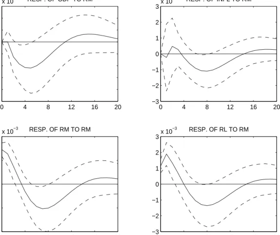
Based on the VAR model, we generate impulse responses of the variables in Zt to a monetary policy shock, which is identified by imposing a triangular orthogonalization. The ordering of the variables implies that an innovation in the money market rate affects the output level and the inflation rate with a lag of one quarter, while the loan rate is affected within the same quarter. Figure 1 displays the impulse responses of the variables to a monetary policy shock. The simulation horizon covers 20 quarters. The solid lines denote impulse responses. The dotted lines are approximate 95% error bands that are derived from a bootstrap routine with 5000 replications.
Our findings conform with the impulse responses reported by Peersman and Smets (2003) and Smets and Wouters (2002) to a monetary policy shock. The output level declines by degrees, reaches a trough after four quarters, and returns to the baseline value subsequently. The reaction of the output level corresponds with the evolution of the output gap. The inflation rate falls slowly and shows a 3The end of our sample period is determined by the switch to the new MFI interest rate
statistics of the European Central Bank (ECB), which entails a structural break in the interest rate data.
4The VAR is estimated with JMulti by L¨utkepohl and Kr¨atzig (2004), which allows to
conduct a variety of test for misspecification and stability. The outcome of the tests – not reported here, but available upon request – have shown that the model is well–specified.
Figure 1: Empirical Impulse Responses 0 4 8 12 16 20 −5 −4 −3 −2 −1 0 1 2 3x 10 −3 RESP. OF GDP TO RM 0 4 8 12 16 20 −3 −2 −1 0 1 2 3x 10 −3 RESP. OF INFL TO RM 0 4 8 12 16 20 −4 −2 0 2 4x 10 −3 RESP. OF RM TO RM 0 4 8 12 16 20 −3 −2 −1 0 1 2 3x 10 −3 RESP. OF RL TO RM
Notes: Orthogonalized impulse responses to a monetary policy shock. The solid lines display impulse responses. The dashed lines are 95% error bands. The horizontal axis is in quarters.
significant decline only after five quarters. Following the trough, which is reached after around eight quarters, it gradually reverts to baseline. The money market rate increases immediately, then declines temporally, and returns to the baseline value subsequently. The loan rate follows a similar pattern as the money market rate, but the reaction is less pronounced.
3.2
Methodology
As in Rotemberg and Woodford (1998) and Christiano, Eichenbaum, and Evans (2005) we estimate the parameters of the log–linearized model by matching its the-oretical impulse responses to a monetary policy shock with the empirical impulse responses. The theoretical model can be summarized by the following matrix representation:
Γ0Xt = Γ1Xt−1 + Ωzzt+ Ωϑϑt, (31) where Xt is the state vector, zt is a vector of shocks and ϑt is a vector of expec-tational errors that satisfy Etϑt+1 = 0 for all t. The matrices Γ0, Γ1, Ωz and Ωϑ contain the structural parameters of the model (Sims, 2001).
The closed loop dynamics of the model, which serves as a starting point to generate impulse responses, is given by:
Xt(%) = ΘX(%)Xt−1+ Θz(%)zt, (32) where the rational expectations equilibrium is solved by using the method devel-oped by Sims (2001). For the matching of the impulse responses, we estimate the following set of parameters:
%= (h θ ω τ δ φπ φYˆ),
by minimizing a distance measure between the theoretical impulse responses and the empirical impulse responses. The remaining parameters were calibrated ac-cording to estimates typically found in the literature (see table 1). The distinc-tion between calibrated and estimated parameters is motivated by the fact that we wanted to estimate only those parameters, which are either sources of real rigidities (h) and nominal frictions (θ, ω, τ), or policy rule parameters (δ, φπ,
Table 1: Calibrated Parameters
Parameter Symbol Calibration
Discount factor β 0.99
Risk aversion σ 1.00
Monopoly power of firms 1/² 1/11 Production function α 0.75 Labor supply elasticity η 2.00
The optimal estimator of % minimizes the corresponding distance measure
Jopt(%) (Christiano, Eichenbaum, and Evans, 2005):
J = min % ³ ˆ Ψ−Ψ(%) ´0 V−1³Ψˆ −Ψ(%)´, (33) where ˆΨ denote the empirical impulse responses, Ψ(%) describe the mapping from
% to the theoretical impulse responses and V is the weighting matrix with the variances of ˆΨ on the diagonal. The minimization of the distance function implies that those point estimates with a smaller standard deviation are given a higher priority.
3.3
Minimum Distance Estimation
Table 2 summarizes the estimated set of parameters ˆΨ that minimize the distance measure. The corresponding impulse responses are shown in Figure 2 together with the empirical impulse responses.
Concerning the Taylor rule, we find that interest rate smoothing is impor-tant, that the output gap turns out to be insignificant and that the central bank positively reacts to the expected inflation rate in t+ 1.
The estimated degree of habit formation is very substantial and seems to indicate that the hump shaped response in the output gap to a monetary shock seems to be mainly driven by habit in consumption itself. This estimate seems to validate the claim of Rudebusch and Fuhrer (2005) that the degree of forward– lookingness in consumption is small.
The degree of Calvo pricing is - compared with other studies - relatively low and implies that prices are fixed on average for half a year. Rule-of-thumb price
Figure 2: Theoretical Impulse Responses 0 4 8 12 16 20 −5 −4 −3 −2 −1 0 1 2 3x 10 −3 RESP. OF GDP TO RM Simulated GDP Estimated GDP 0 4 8 12 16 20 −3 −2 −1 0 1 2 3x 10 −3 RESP. OF INFL TO RM Simulated INFL Estimated INFL 0 4 8 12 16 20 −4 −2 0 2 4x 10 −3 RESP. OF RM TO RM Simulated RM Estimated RM 0 4 8 12 16 20 −3 −2 −1 0 1 2 3x 10 −3 RESP. OF RL TO RM Simulated RL Estimated RL
Notes: Orthogonalized impulse responses to a monetary policy shock. The solid lines display impulse responses. The dashed lines are 95% error bands. The horizontal axis is in quarters.
Table 2: Parameter Estimates
Parameter Symbol Estimate t-value Habit formation h 0.89 47.32 Price stickiness θ 0.41 1.98 Rule-of-thumb pricing ω 0.75 18.03 Loan rate stickiness τ 0.40 11.54 Taylor rule: smoothing δ 0.72 13.57 Taylor rule: output gap φYˆ 0.02 0.13 Taylor rule: inflation φπ 1.07 5.25
Notes: The value function is 44.20 with a probability of 0.99824. The probability is calculated by employing a Chi–Squared distribution with 75 degrees of freedom. The standard errors are calculated as the square root of the diagonal elements of the inverted Hessian matrix resulting from the optimization of the value function.
setters amount to 75 percent of the firms.
The significant estimate forτ reveals that the banking industry plays a mean-ingful role in propagating monetary shocks via the cost channel. The degree of loan rate stickiness τ was estimated to be 0.40, which implies that loan rates are fixed on average for half a year. This result can be considered as a contribution to literature as we extend earlier findings by Ravenna and Walsh (2006) who only model the banking industry as a neutral conveyor of monetary shocks. Their model of the banking industry can be regardedas a special case of our model with
τ = 0.
Additionally, the significant estimate of κ is evidence for the existence of a cost channel in the euro area.
4
Conclusion
This paper has addressed the cost channel of monetary transmission and the role of the banking industry in the euro–area by using aggregate data. Our motivation originates from two sources. Empirically, VAR models show that the loan rate follows the policy rate after a monetary policy shock, but the adjustment is less pronounced. Theoretically, the standard New Keynesian model (as for example presented in Woodford, 2003, ch. 4) does not explicitly model a banking industry.
Therefore we have extended a New Keynesian model including habit formation and rule–of–thumb setters to allow for a more realistic description of financial intermediation. Related literature is in particular Ravenna and Walsh (2006) and Chowdhury, Hoffmann, and Schabert (2006). Empirically, we have evaluated the existence of a cost channel and the role of the banking industry by matching the theoretical impulse responses with the empirical impulse responses to a monetary shock. Our findings suggest that there is clear evidence for the existence of a cost channel in Europe working alongside the interest rate channel. This result is consistent with Chowdhury, Hoffmann, and Schabert (2006), who draw similar conclusions based on single equation GMM estimates for the G7 countries.
Additionally our findings suggest that the cost channel in the inflation ad-justment equation are not only driven by loan demand, but additionally by loan supply factors. This result is a contribution to literature and extends earlier find-ings by Ravenna and Walsh (2006) who only model the banking industry as a neutral conveyor of monetary shocks.
References
Barth, M. J., and V. A. Ramey (2000): “The Cost Channel of Monetary
Transmission,” NBER Working Paper 7675, National Bureau of Economic Re-search.
Calvo, G. A. (1983): “Staggered Prices in a Utility–Maximizing Framework,”
Journal of Monetary Economics, 12, 383–398.
Chowdhury, I., M. Hoffmann, and A. Schabert (2006): “Inflation
Dy-namics and the Cost Channel of Monetary Transmission,” European Economic Review, forthcoming.
Christiano, L. J., M. Eichenbaum, and C. Evans(2005): “Nominal
Rigidi-ties and the Dynamic Effects of a Shock to Monetary Policy,” Journal of Po-litical Economy, 113, 1–45.
Clarida, R., J. Gali, and M. Gertler (1999): “The Science of Monetary
Policy: A New Keynesian Perspective,” Journal of Economic Perspectives, 37, 1661–1707.
Freixas, X., and J.-C. Rochet (1997): Microeconomics of Banking. MIT
Press Cambridge, Massachusetts, Massachusetts.
Gali, J., M. Gertler, and J. D. Lopez–Salido(2001): “European Inflation
Dynamics,” European Economic Review, 45, 1237–1270.
L¨utkepohl, H., and M. Kr¨atzig (eds.) (2004): Applied Time Series
Econo-metrics. Cambridge University Press, Cambridge.
Peersman, G., andF. Smets(2003): “The Monetary Transmission Mechanism
in the Euro Area: More Evidence from VAR Analysis,” in Monetary Policy Transmission in the Euro Area, ed. by I. Angeloni, A. Kashyap,and B. Mojon. Cambridge University Press (forthcoming).
Ravenna, F., and C. E. Walsh (2006): “Optimal Monetary Policy with the
Rotemberg, J. J., and M. Woodford (1998): “An Optimization–Based Econometric Framework for the Evaluation of Monetary Policy: Expanded Ver-sion,” Technical Working Paper 233, National Bureau of Economic Research.
Rudebusch, G., and M. Fuhrer (2005): “Estimating the Euler Equation for
Output,” Journal of Monetary Economics, 51, 1133–1353.
Sims, C. A. (2001): “Solving Linear Rational Expectations Models,”
Computa-tional Economics, 20, 1–20.
Smets, F., and R. Wouters(2002): “An Estimated Stochastic Dynamic
Gen-eral Equilibrium Model of the Euro Area,” Journal of the European Economic Association, 1(5), 1123–1175.
Woodford, M. (2003): Interest and Prices: Foundations of a Theory of