Capital, Interest, and Aggregate Intertemporal Substitution

(1)

NBER WORKING PAPER SERIES

CAPITAL, INTEREST, AND AGGREGATE INTERTEMPORAL SUBSTITUTION

Casey B. Mulligan Working Paper 9373

http://www.nber.org/papers/w9373

NATIONAL BUREAU OF ECONOMIC RESEARCH 1050 Massachusetts Avenue

Cambridge, MA 02138 December 2002

I appreciate the comments of Olivier Blanchard, Robert Barro, John Campbell, Austan Goolsbee, Lars Hansen, Jason Hwang, Bob Lucas, Andrew Scott, Mike Woodford, GSB macro lunch eaters, participants at the 2001 European Meeting of the Econometric Society, seminar participants at Chicago, M.I.T., B.U., and Harvard, and the research assistance of Fabian Lange and Justin Marion. This research was made possible by financial support from the Alfred P. Sloan Foundation under their Research Fellowship program. The views expressed herein are those of the authors and not necessarily those of the National Bureau of Economic Research.

© 2002 by Casey B. Mulligan. All rights reserved. Short sections of text, not to exceed two paragraphs, may be quoted without explicit permission provided that full credit, including © notice, is given to the source.

(2)

NBER Working Paper No. 9373 December 2002

JEL No. E21, H30, E22

ABSTRACT

Financial economics research has suggested that expected returns are not the same across assets, and that their movements over time are not simply described or explained. I argue that this suggestion has implications for the study of substitution over time – namely that “the” interest rate in aggregate theory is not the promised yield on a Treasury Bill or Bond, but should be measured as the expected return on a representative piece of capital. Furthermore, tax policy changes can be used to distinguish intertemporal preferences (a.k.a., the supply of savings) from the demand for capital, and to distinguish Fisherian from non-Fisherian interpretations of consumption-interest rate comovements. I so measure the interest rate using U.S. national accounts data, and find consumption growth to be both interest elastic and forecastable with tax and interest rate variables. In other words, standard proxies for “the intertemporal marginal rate of substitution” and for “the marginal product of capital” move together, once we allow for taxes, even though both fail to be significantly correlated with any particular financial asset’s return.

Casey B. Mulligan Department of Economics University of Chicago 1126 East 59th_Street Chicago, IL 60637 and NBER [email protected]

(3)

macroeconomics, and are pretty important in other fields as well. In studying these behaviors, there is a long tradition of conceptually distinguishing the supply from demand for capital or, in modern terminology, distinguishing intertemporal preferences from the technology of accumulation. In theory, “the interest rate” coordinates these two sides of the market. But there are many types of capital and financial assets in the U.S. economy – which asset’s return should have the closest connection with savings behavior? A bond return? A stock return? The return on the capital stock? The purpose of this paper is to reexamine the relation between consumption growth and “the interest rate,” with special attention to these questions. The results are some very different conclusions about aggregate consumption growth: it is interest elastic, and forecastable.

Most previous studies of interest rates and savings, and investment, measure the return on a bond (or another particular financial asset) for the purpose of predicting savers’ behavior, and only measure the income generated by the capital stock for the purpose of studying firm behavior (eg., Feldstein and Summers 1977, or Auerbach 1983). There are two understandable reasons for preferring the bond return in a study of consumer behavior: (a) a lot of people hold bonds, bank deposits, or similar securities in their portfolio, and (b) there are a variety of market distortions that could drive a wedge between the expected returns on bonds (or another financial asset) and aggregate capital, even when the former is in theory more closely associated with consumption growth. For example, in theory, capital taxation, a rising supply price of investment goods, and/or imperfections in the financial intermediation process could drive a wedge between the return on capital and the return on the financial assets savers hold in their portfolio.

While this approach suggests that financial asset returns should have a closer link with consumption growth than does capital income, it does not recognize that expected financial asset returns fluctuate over time in a way that varies across financial assets, and cannot be explained by the covariance structure of financial returns and consumption growth. If the expected return on one

(5)

Capital, Interest, and Substitution - 2

financial asset rises, and the expected return on another falls, what should happen to consumption growth? The approach in my paper is not to “explain” asset price differentials, but to suggest that whatever explains them also causes the expected return on a particular financial asset to depart from the expected return on aggregate capital, while it is the latter driving aggregate consumption growth. I illustrate this point with a state-dependent utility model of aggregate intertemporal substitution, and show how the correlation between expected consumption growth and the “risk free” rate can be positive or negative, depending on the importance of shocks to the demand for capital relative to the shocks creating asset price differentials. Hence, neither the sign nor magnitude of the intertemporal elasticity of substitution (hereafter, IES) is informed by this correlation. Another correlation – the correlation between expected consumption growth and the expected return on the aggregate portfolio – gives much more information in this regard, so the bulk of my paper is devoted to building a time series on capital’s return (Section II), showing how that time series is very different from the time series of bond returns, and using that series to estimate an elasticity of aggregate intertemporal substitution (Section IV).

Capital income can be used to measure “the interest rate” driving consumer behavior, without denying that there are distortions driving a wedge between the return on capital and the return earned by a saver. For example, Section III builds a time series for the aggregate rate of capital taxation, and shows that consumption growth has a closer empirical relation with the after-tax return than the pre-after-tax return. I show how high capital income after-tax rates are associated with low rates of consumption growth, and use the tax rate series to decompose expected return fluctuations into those deriving from the productivity of capital, and those deriving from the willingness of people to save. Furthermore, I show how the comovement of consumption growth, interest rates, and capital tax rates can be used to mitigate the problems deriving from capital price mismeasurement, and to distinguish intertemporal substitution interpretations of the correlation between consumption growth and interest rates from NonFisherian interpretations.

The intuition motivating my approach can be seen by a simple analogy. If we were interested, say, in the willingness of consumers to substitute food for other goods, then we should look at the correlation between food expenditure and a food price index. This correlation would have little relation with the correlation between food expenditure and the price of carrots, unless there were a perfect correlation between the price of carrots and the price of all other foods. There may be theories of food demand implying that the price of carrots is always in the same proportion

(6)

1_{Or, for that matter, whether savings behavior is measured according to consumption} growth or the savings rate. Boskin (1978) and many other studies of the interest elasticity of savings measured “the interest rate” according to financial asset returns.

2_{“But the economist has little concern with particular incidents in the lives of individuals} ...the variety and fickleness of individual action are merged in the comparatively regular

aggregate of the action of many.” Alfred Marshall, Principles of Economics, III.iii.5.

to other food prices, but if in fact there were something moving the price of carrots apart from the prices of other foods, then a price index for all foods is needed. By analogy, my paper compares consumption growth with the return on a large portfolio of capital assets, rather than the return on a particular asset.

Hall (1988, p. 353) states: “It simply cannot be said that the relation between the real return and the rate of change of consumption supports strong intertemporal substitution.” His basic characterization of aggregate data is widely accepted, so some have responded to Hall’s findings by arguing that intertemporal substitution is more readily seen in microeconomic data. For example, Attanasio and Weber (1993) find building society deposit rates to relate differently with aggregate consumption growth than with cohort-specific consumption growth. Vissing-Jorgensen’s (2001) results suggest that consumption growth is correlated with expected stock returns in the population of households owning stocks, and that consumption growth is correlated with expected bond returns in the population of households owning bonds. Gross and Souleles (2001) study the credit card debt of households who have credit cards and maintain a balance, and show how households hold less credit card debt when the credit card interest rate is higher. Their finding is consistent with a variety of hypotheses, and one of them is that each household adjusts its consumption growth in response to the interest rate it faces as supposed by the intertemporal substitution hypothesis.

According to one view, my study is not related to the question of whether consumption should be studied at the individual or aggregate levels. In fact I study aggregate consumption, but the main issue raised here is how to measure and decompose “the interest rate” for the purposes of studying the timing of consumption, an issue which is also relevant for those studies measuring consumption at the individual level.1_{A more zealous (and Marshallian}2_{) view has the aggregate,} rather than individual, relationship between consumption growth and interest rates as the one of direct relevance for aggregate questions (such as the aggregate effects of a war, or a tax on all capital goods). Since economic theory alone does not tell us whether the aggregate relationship is more

(7)

3_{For example, the aggregate relationship could be a complicated function of the} microeconomic relationship, as in the models sketched out by Attanasio and Weber (1993, p. 632). Or there might be a simple and stable relationship among the aggregates, while various individuals are substituting on different margins and to different degrees, as in a model of Summers (1982).

stable, or less stable, or of the same magnitude, as the microeconomic relationships,3_{direct evidence} on the aggregate relationship is needed. I show how intertemporal substitution of consumption is readily seen in the aggregate data (even through the lense of a representative-agent no-borrowing-constraint model), as long as “the interest rate” and its components are measured at a more aggregate level than in the previous literature. Exactly how the aggregate relationships found in my study (or previous aggregate studies) derive from individual behavior, and whether the aggregate or individual behavior is more reliable for policy purposes, is another question.

II. Measures of the Return on Capital

II.A. Asset Prices and Intertemporal Substitution in a State-Dependent Utility Model

Consider a dynamic economy with only a single asset in positive net supply – “capital.” Capital earns a time-varying and stochastic return. In each period, there are S possibilities for capital’s return, which I index s = 1, ..., S. A dollar of investment in year t-1 yields state s gross return M_ts / ems%µt in year t, which I decompose into a deterministic component µ_t and a stochastic component ms_{. The states are ordered so that the stochastic component rises with}_s_:_m1_<_m2_<_m2 < ... < mS_{. From the point of view of year}_t_{-1 (and earlier), the probability of state}_s_{occurring in year}

t is πs_{. I let}_E

t-1(@) denote mathematical expectations with respect to this probability distribution. I normalize the state-specific returns so that Et-1(m) = 0, and Et-1(ln Mt) = µt.

The representative consumer owns the capital, and it is his only source of income. He consumes at each point in time, in the amount ct in year t. His preferences are defined over

consumption processes {c_t}, and are recursive over time. In order to characterize his optimal consumption plan, I use the following Bellman equation:

(8)

4_{Utility is also time-dependent, because the preference parameters {α}s_{} and ρ vary with}_t_.

5_{The parameters {α}s_{} can be interpreted as “subjective probabilities.” Alternatively,}

interpret the program (1) as a reduced form of a model with objective probabilities, and time-and state-specific household production functions. For example, in the two-period case with σ=1, a household’s utility would be lnz1 % βj , where z1 is household production in

N s'1

πs_ln_zs

2

period 1, and z₁s_{household production in period 2 and state}_s_{. Household goods are produced}

from market purchases according to the state-dependent function z₂s ' (c₂s)αs_/_πs. v_t&1(k_t&1M_t&1) ' max

c_t_&₁,k_t

c_t&1(σ&1)/σ % e&ρt&1 _eFt&1[lnvt(ktMt)] (σ&1)/σ σ/(σ&1)

s.t. k_t ' k_t&1M_t&1 & c_t&1 F_t&1(x) / '

s

αs_t&1xs

(1)

By using the Bellman equation (1) to characterize optimal consumption plans, I have assumed that the representative agent’s preferences are of the recursive variety studied by Epstein and Zin (1989), with constant intertemporal elasticity of substitution σ > 0 and (time-varying) rate of time preference ρ. The Bellman equation (1) represents the piece of the optimal plan where the consumer chooses current consumption ct-1, and the amount of capital kt to carry into the next period, without

knowledge of the capital returns be realized years t and later, but knowing the capital returns realized in the current year t-1 and knowing the entire time sequences of the preference parameters. Three economic ideas are separately embodied in the Bellman equation (1). The first two are “risk aversion” and “intertemporal substitution,” which are also emphasized in the work by Hall (1988) and Epstein-Zin (1989). Epstein and Zin point out that equation (1) has logarithmic “expected utility” as a special case in the limit as σ approaches one, so that the IES approaches the inverse of the coefficient of relative risk aversion. The third economic idea embodied in (1) is “state dependence” because the “expectation” Ft-1(@) is defined as Ft&1(x) / ' , where the

s

αs_t&1xs

parameters {αs_{} sum to one across states, but vary over time and are not necessarily the same as the}

mathematical probabilities {πs_}.4_{State-dependent utility is perfectly “rational,”}5_{but it is avoided} in much economic analysis – and embraced here – because it puts fewer restrictions on the prices

(9)

φσ_t_&&₁1 ' 1 % e&σρt&1 _φ te

F_t_&₁(lnM_t)σ&1

6_{Equation (2) can be derived by first guessing that each of the value functions}_v

t(x) takes

the form ntx, where nt is a constant that depends only on the time sequences {µi,ρi,{α , s

i} s s'1}4i't

as described recursively below:

Second, the first order conditions can be used to calculate cts/ct-1. Third, sum across states weighting by the objective probabilities.

E_t&1 ln ct

c_t_&₁ ' σEt&1(lnMt) & ρt&1 % (σ&1)'

S s'1

(αs_t&1&πs₎_ms ₍₂₎

lnL_t ' E_t&1(lnM_t) % lnF_t&1(1/m) % lnφ_t ₍₃₎

of contingent claims. The purpose of my model is to explore the intertemporal substitution implications of departures from the relationships implied by the consumption-based asset pricing theories developed by Lucas (1978) and Breeden (1979), and extended by Epstein and Zin (1989), without actually explaining the reasons for those departures. The question of which return predicts consumption growth is more interesting when the expected returns on various assets are imperfectly correlated as they are in the model (1), just as the question of how to put food prices in a food demand equation is more interesting when the prices of the various foods are imperfectly correlated.

A simple expression for expected consumption growth can be derived from (1):6

where Mt is the year t return on capital accumulated in year t-1. The elasticity of expected

consumption growth to capital’s expected return is, holding constant the probabilities and the preference parameters, the constant intertemporal elasticity of substitution σ.

Now consider the relation between expected consumption growth and the gross return L_t on a risk free asset purchased in year t-1 for maturity in year t. The risk free asset is, by assumption, in zero net supply in this economy, but we can price it in the usual manner:

where nt is a constant that depends only on the time sequences{µi,ρi,{α (see footnote 6). s

i} s s'1}4i't

(10)

σ_L ' θ σ % λ(σ&1)

In words, the risk free rate promised in year t-1 for maturity in t depends on (a) capital’s one-period expected return Et-1(ln Mt), (b) the current preference parameters {α , and (c) the combination

s t&1}

S s'1

of future preference and capital parameters embodied in the constant nt. Fluctuations over time in

capital’s expected return create parallel fluctuations of expected consumption growth and the risk free rate, because capital’s one-period expected return Et-1(ln Mt) enters both the risk free rate

equation (3) and the consumption growth equation (2). However, fluctuations over time in the taste parameters do not create parallel fluctuations of expected consumption growth and the risk free rate. Indeed, the taste fluctuations can lead to a negative correlation between consumption growth and the risk-free rate. To see this, first use the model to calculate the coefficient σ_L of a time-series regression of consumption growth on the risk free rate:

The weights θ and λ are complicated functions of time series variances and covariances. I leave it to the reader to show that, when the time-series{µ_t,ρ_t,{αs_t}s_s'1} are mutually independent, both weights are in the interval [0,1], and do not necessarily have to sum to one. Furthermore θ=1 and λ=0 only in the special case that there are no taste fluctuations.

σ = 1 is an interesting special case, because we have σL = θσ and can isolate one of the

reasons why the risk free rate coefficient contains little information about intertemporal substitution. Namely, as seen in equation (2), expected consumption growth responds only to capital’s expected return and to the rate of time preference, while the risk free rate responds both to capital’s expected return and the taste shocks. θ < 1 measures the relative variability of “signal” (ie., the variability of capital’s expected return) to the overall variability of the risk free rate. The time series regression of consumption growth on the risk free rate suffers from a regression bias, because the risk free rate measures capital’s return with error, just as we would expect the regression of food expenditure on the price of carrots to suffer from a regression bias. More generally, the risk free rate coefficient tells us less about intertemporal substitution when the risk free return is driven by “taste” shocks. In the limit of no fluctuations in capital’s expected return, θ=0 and the risk free rate coefficient σP

is a downward biased estimate of (σ-1).

(11)

Taste changes can drive the risk free rate and consumption growth in opposite directions. This occurs because taste changes have opposing wealth and substitution effects on consumption growth. An increased preference for the bad states (modeled, for example, as dα1_=-_d_αS_{>0) drives down the}

risk free rate. This preference change also reduces the “subjective return” on capital (namely, the return featured in equation (1)) without affecting the actual return on capital. The reduced subjective return has the textbook income and substitution effects on capital accumulation. On one hand, consumers cannot afford the old utility level, a wealth effect which by itself reduces current consumption and increases capital accumulation. On the other hand, lowering future marginal utility is more costly in terms of foregone current consumption, which creates a substitution effect lowering capital accumulation. The wealth effect dominates with σ < 1 and the intertemporal substitution effect dominates with σ > 1.

Hall (1988), Summers (1982), and others studying the effect of the Treasury Bill return on consumption growth have also replaced the T-bill return with expected returns on other assets, such as those on savings deposits, long term bonds, or a particular stock portfolio. But this is like removing the price of carrots from the food expenditure regression, and replacing it with the price of milk, the price of apples, or the price of bread – none of these exercises is the same as using all of the food prices in a food price index. More precisely, my model can generate a pricing equation for any asset and, as long as the asset is not the same as (or a large fraction of) the aggregate capital stock, the pricing equation will be like equation (3): a combination of capital’s expected return and the preference parameters. Changes in the preference parameters cause a departure between the expected return on capital and the expected return on savings deposits, or long term bonds, IBM’s share price, etc., and the regression of consumption growth on any one of the expected returns will suffer from a regression bias. To the extent that σ differs from one, the bias may be even worse for the reasons explained in the context of the risk free rate.

In summary, the state-dependent utility model implies that capital demand fluctuations cause parallel movements in the expected returns on all assets, while preference fluctuations have different effects on the various asset returns. If preference shocks are important, then the coefficient from a time series regression of consumption growth on an asset’s expected return is not the IES, and is not necessarily positive, unless the asset’s risk properties are similar to the risk properties of the aggregate capital portfolio. The rest of the paper uses the national income and wealth accounts to measure the expected return on the “aggregate capital stock.” The national accounts are used for

(12)

7_{“Expected obsolescence implicitly enters into BEA estimates of depreciation through} shorter asset lifetimes and through the retirement pattern previously used.” (Fraumeni 1997, p. 9). The BEA does not estimate asset-and-year-specific depreciation rates (the aggregate depreciation rate does change over time according to composition of the capital stock); several econometric studies have failed (eg., those cited by Fraumeni 1997, p. 13) to reject the

hypothesis that asset-specific depreciation rates are constant over time.

8_{At least for the postwar years, Gordon (1990) and others present evidence calling into} question the accuracy of the BEA index. Similar questions may be just as applicable prior to 1947, although I am not aware of a systematic study of this issue. Also, Cochrane (1991) and others in the finance literature have shown how capital gains on financial assets like the NYSE portfolio are much more volatile than the returns on investment implied by the national accounts. Perhaps this is a weakness of the national accounts (eg., they may exclude the “adjustment costs” emphasized in Cochrane’s study), or perhaps the financial capital gains derive from the kinds of “preference” changes modeled above, and hence should be ignored in a study of the timing of aggregate consumption.

two reasons: they have the advantage of including residential structures, the physical capital of noncorporate enterprises, and other assets on which owners of marketable stocks and bonds have no claim, and they can be readily reconciled with capital tax information.

II.B. Capital Returns as Measured in the National Accounts

The return on a capital asset can be decomposed into a rental rate and a capital gain. Capital gains might result from a variety of forces, including aging, obsolescence and changes in the demand for the asset’s services. To the extent that these gains are unanticipated, they do not in theory affect expected consumption growth. Perhaps one advantage of the national accounts (for my purposes) is that their concept of depreciation includes expected aging and obsolescence,7_{and hence may} provide an estimate of a big component of the expected capital gains. In principle, one could test the hypothesis that, other than BEA’s estimate of depreciation, aggregate capital gains are unforecastable, although perhaps the BEA’s estimate of the prices of equipment, housing, and other assets are not good enough for such a test.8_{To begin the analysis, it is presumed that aggregate} capital gains, net of BEA depreciation, are unforecastable, so that capital’s pre-tax expected return might be measured according to the amount of capital income net-of-depreciation that is earned per dollar of capital.

Figure 1's solid line displays a measure of aggregate annual capital rental rates: capital income net of depreciation per dollar of capital in place at the beginning of the year. Capital is

(13)

9_{Data sources are detail in Appendix II.}

10_{Government net product is equal to the compensation of government employees,} because, as explained by Parker et al (1995, p. 36), the national accounts assume that

government assets (other than those used by government enterprises selling their output in the marketplace) yield no services in production beyond their depreciation.

11_{These two steps implicitly assume that capital and labor income accrue in the same} shares in three sectors – the nonproprietary sector, the proprietary sector, and the foreign sector. My formula for pre-direct-tax private sector capital income is (NI-Yg-NFI)[1-Wp/(NI-Wg-Ys)],

where Ys is proprietors’ income, NI is national income, NFI is net factor income from abroad, Wp

is the private employee compensation of domestic residents, and Wg is the labor compensation of

domestic government employees.

measured as proportional to the BEA’s (2000) fixed assets valued at current cost, and is aggregated for private residential and nonresidential sectors.9_{Note that the capital measured is employed} domestically (including foreign-owned capital), includes owner-occupied housing, excludes consumer durables, and excludes the government sector. Current cost capital is not the same as book value, because the former aggregates real investment flows, and the latter aggregates investment expenditure flows. Capital income is measured accordingly, in two or three steps. First, income accruing to agents with their factors domestically and privately employed is calculated by subtracting net government product10_{and net factor income from abroad from national income.} Second, this income is multiplied by one minus labor’s share of non-proprietors’ private national income, in order to obtain an estimate of the income pre-direct-taxes going to domestically employed capital.11_{Third, capital income is adjusted for direct and/or indirect taxes. The third step} is skipped in the construction of the series shown in the Figure in order to display the years prior to 1929, and is skipped by Feldstein and Summers (1977), in which case the result is a measure of capital’s rental rate before direct taxes, but after indirect taxes. If the third step adds property income tax revenue back into capital income, as suggested Feldstein, Dicks-Mireaux, and Poterba (1983), the result is a capital rental rate before all taxes, and perhaps the better proxy for the marginal product of capital. Subtracting direct capital taxes in the third step (and adjusting the timing of the property taxes – see below) gives an estimate of the rental rate after direct and indirect capital taxes. As I show below, my contribution is to make this final calculation (an extension of those made by Griliches and Jorgenson (1966, p. 58)), relate after-tax capital rental rates to consumption and financial asset returns, and to interpret these relationships in terms of aggregate

(14)

12_{Like Shiller (1989) and others studying bond returns for a long historical time period, I} measure commercial paper, rather than Treasury Bill, yields because of the available of long time series for the former.

intertemporal substitution.

My pre-direct-tax capital rental measure ranges from 3.7 to 12.5 percent. Figure 1 also graphs, as a dashed line, the time series for ex poste real returns on commercial paper (measured as the difference between the prior year promised annual nominal yield minus GDP deflator inflation since the prior year).12_{The two series are correlated -0.24. Just as important, the real paper yields} vary much more over time than do the capital rental rates – the standard deviation of the former exceeds that of the latter by a factor of 3 or 4!

(15)

Figure 1 Capital Rental Rates Compared with Commercial Paper Yields (Note: for the purposes of illustration, paper yields are truncated at +/- 0.12)

The real paper return shown in Figure 1 may significantly differ from the anticipated yield because inflation is different than anticipated, and in most theories it is the anticipated yield that determines consumption growth. Hall (1988) deals with this in two ways: (1) looking at longer time-averages of real yields and, implicit in his two stage estimation of consumption growth equations, (2) working with forecasted real returns. I follow Hall here, both in regards to capital rental rates and real paper yields. We already suspect from Figure 1 that anticipated capital rental rates may differ significantly from anticipated real paper yields. For example, real paper yields are consistently negative during the 1940's, while 1940's capital rental rates are fairly typical by postwar standards. If we average Figure 1's data over five year intervals, as Hall did with his data, we see that the two time-averaged return measures are correlated -0.28. The time-averaged real paper

(16)

13_{Although capital income in this case should be calculated with the depreciation of the} portfolio, and not the national accounts capital stock depreciation/

yields fluctuate much more than, and are hardly associated with, the capital rental rates; a time series regression of capital’s rental rate on the real paper yield (both series time-averaged) yields a coefficient of -0.08.

Figure 1 also shows that the postwar pre-tax rental rate is similar to, or even lower than, the prewar rates. This long-term comparison, and hence those statistical analyses below that use the long-term data, is sensitive to exactly how the capital stock is measured. BEA’s current cost capital concept is the product of the real capital stock and the price of capital. In other words, a rental rate based on this measure gives the rent that would be earned on a $1 portfolio where that portfolio held the economy’s various capital assets in the proportion as they are in the capital stock. Let’s denote that rental rate as R/(pk), where R aggregate capital income, p is the average price of capital, and k is the real capital stock. But what about a $1 portfolio holding the economy’s various capital assets in the proportions as they are in investment? We might also estimate this portfolio’s rental rate as R/(pk),13_{but with}_p_{as the average price of new investment goods. According to the BEA data, the} price of investment has declined a lot more than the price of capital (perhaps because investment has been shifting toward goods with low and falling prices?), and the difference is particularly dramatic 1929-33. The differences are large enough that, when measured according to the investment price, the pre-direct-tax rental rate trends upward, and is significantly higher after the war. It is not clear whether intertemporal choice theory provides any guidance as to which rental rate to use, so most of the analysis in this paper follows previous studies of capital returns and uses the current-cost based measure (p is the price of capital), reporting a few specifications with “the interest rate” calculated as the average of the two rental rate measures.

II.C. A First Comparison of Consumption and Capital Rental Rates

Figure 2 compares average annual per capita consumption growth with average annual capital rental rates, where each observation is a five year period. Figure 2 is constructed exactly like Hall’s (1988) scatterplot, with one important difference and one minor difference. The important

(17)

-0.02 0 0.02 0.04 0.06 0.08 consumption growth 0.045 0.05 0.055 0.06 0.065 0.07

rental rate, after tax 1931-35 1936-40 1941-45 1946-50 1951-55 1956-60 1961-65 1966-70 1971-75 1976-80 1981-85 1986-90 1991-95 1996-

(18)

14_{Recall that the capital rental rate shown in Figure 1 does not include a subtraction for} direct taxes.

15_{That these differences are relative minor is carefully demonstrated below, and in the} Appendix I.

difference is that my interest rate measure is the (after-direct-tax14_{) capital rental rate rather than} Hall’s Treasury bill return. The minor difference15_{is that I also include the years 1941-45 and} 1984-99. Using the capital rental rate makes a huge difference, because we see an obvious positive relationship between consumption growth and “the interest rate.” The least squares regression line has slope 2.06 (s.e.=0.85).

III. Measures of Capital Taxation and After-Tax Returns

Capital taxation is related to intertemporal substitution for at least three reasons. First, the incentive to save is, in many economic models, the combination of the return on assets and the taxes owed on those returns. Second, it may be that changes in the capital income tax rate are sources of fluctuations in the after-tax return on capital that are not associated with preference shifts and other determinants of consumption growth. In other words, capital taxation can help identify a structural relationship between consumption growth and returns even though the very logic of general equilibrium models implies that the observed relation between consumption growth and returns is a reduced form one. Third, capital tax incidence is one of the reasons why it is important to have a good estimate of the aggregate IES, and using the capital tax data can help us directly answer the incidence question while at the same time provide better estimates of the IES. Along these lines, this section constructs and interprets time series of tax variables that can be related to aggregate consumption. Readers interested in the IES estimates, and willing to accept my interpretation of the tax variables, may want to skip immediately to Section IV.

III.A. Capital Taxes and Rental Rates

Hall (1988) measures an after-tax real return on Treasury bills by multiplying (one minus) Barro and Sahasakul’s (1983) annual marginal federal personal income tax rate by the nominal Treasury bill yield, and subtracting inflation. It is unclear whether Hall correctly quantified these

(19)

16_{The share of personal income taxes included as a “capital tax” is measured as one minus} labor’s share of AGI. The “labor income” components of AGI are assumed to be wages & salaries, pensions and annuity income included in AGI, taxable social security benefits, taxable IRA distributions included in AGI, and unemployment compensation included in AGI. In an earlier draft of the paper, I reported very similar IES estimates by measuring capital’s share of personal income taxes as one minus labor’s share of personal income.

taxes for the purposes of understanding aggregate consumption, since the tax code treats assets and taxpayers differently. If capital returns were measured as the return on a particular financial asset, such as a Treasury bill or commericial paper, and we were to include taxes in the analysis, we would have to decide whether and how the owners of that asset were liable for taxes at each point in time and adjust the pretax returns accordingly.

Aggregate tax calculations based on the national accounts are more straightforward, since we just subtract aggregate direct capital tax revenue from aggregate capital income (which, since derived from national income, already subtracts indirect business taxes), although there is still the question of how to price the capital stock. With Figure 1's pre-direct-tax capital rental rate shown (solid line) as a benchmark, Figure 3 displays as a dash-dot line the result of subtracting federal, state, and local corporation income taxes and a share of personal income taxes from capital income.16 Both the solid and dash-dot lines display rental rates calculated using the price of capital, but the dashed line shows the after-tax rental rate calculated using the price of investment (and is available only since 1930). As a result, Figure 3 displays two very different stories about the effects of corporate and personal income taxation, which were so much more important after 1940 than before. According to the dash-dot and solid series, pre-tax rentals were similar, and after-tax rentals significantly lower, after the war when capital taxation was significant. According to the dash-dot series, after-tax capital rentals show relatively little decrease, and perhaps is more consistent with the conclusions that capital does not bear much of the burden of the capital income tax, and consumption growth is interest elastic.

(20)

17_{The estimates in this section and in the Appendix I were made possible by ongoing} research with Justin G. Marion. Some of those results are reported in Mulligan and Marion (2000).

Figure 3 Capital Rental Rates

III.B. Capital Tax Revenue Sources

There are many kinds of capital, and many forms of capital taxation. One approach might be to explicitly model this complexity, at risk of distracting from the main issue of this paper – the aggregate IES. Instead we17_{follow Griliches and Jorgenson (1966, p. 58), Feldstein, Dicks-Mireaux,}

(21)

18_{Lucas (1990) uses a similar method to measure the capital tax rate for 1985 (0.36).}

Mendoza et al (1994) and Lucas (1990) apparently count revenue according to the year it arrives in the Treasury and therefore in the government budget. For example, a personal income tax payment made April 15, 1985 for the 1984 tax year would count as 1984 in my calculations and as 1985 in the Mendoza et al/Lucas calculations.

τ_t ' Tt%Pt%1 R_t%P_t

T_t / (corporate inc tax revenue)

% (estimated personal capital inc tax revenue)

% (property tax revenue)

(estimated personal capital inc tax revenue) /

(nonlabor inc share of AGI) (total IIT revenue)

and Poterba (1983), Lucas (1990), and Mendoza et al (1994) and attempt to construct annual

measures of the rate τt of taxation of a representative piece of capital’s date t income. More

specifically, we use the following formula:

where Rt is date t aggregate capital income before direct taxes and after indirect taxes, and Pt is

property tax revenue received by the government in year t. These are similar to Mendoza et al’s

measures, with four exceptions (i) our definition of capital income is slightly different, (ii) we added property taxes back into the aggregate capital income (see the denominator, and also Feldstein,

Dicks-Mireaux, and Poterba 1983), and (iii) we count tax revenue according to the tax year.18_On

point (iii), we have used IRS records to measure personal and corporate tax liabilities by tax year. On point (iv), when we have data on aggregate property tax revenue (1929-), we assume that property tax liabilities accrue in the year prior to their arrival at the treasury, as indicated in the formula above. Adjustments corresponding to (iv) were not made for the after-tax rental series shown in Figure 3 because they span the entire century but, as indicated below, will be made for statistical calculations involving the period 1929-. Hence, given our definition of the tax and rental rates, the tax rate is the percentage gap between the after tax rental rate and the rental rate before direct and property taxes.

(22)

19_{We conjecture that property tax assessors did not adjust the dollar value of their} assessment during the 1930's, when the overall price level and dollar incomes were falling, which is why aggregate property tax revenue was pretty stable in dollar terms and such a large fraction of aggregate capital income.

Figure 4 Capital Income Tax Revenues by Major Type, 1929-97 (as a share of aggregate capital income, before direct and property tax)

personal, and property tax components. We see how the corporate income tax accounts for most of the tax rate fluctuations, with the exception of the 1930's when corporate and personal income tax revenues were few and property tax revenues were substantial relative to capital income.19

(23)

are an important ingredient in my analysis, it is worth understanding some of the history of those tax changes. The major ones are associated with real, although sometimes passive, changes in public policy. For example, the higher levels since 1940 derive from the well known increase in government revenue’s share of GDP, part of which was financed with the introduction and growth of corporate and personal income taxation. The reduction at the end of the war derives from reductions in corporate and personal income tax rates, and probably in part from legislative adjustments of nominal tax code to the higher postwar price level. Federal corporate income tax rates increased from 38 to 52 percent 1949-52, contributing to the rapid increase in my corporate measure during those years. Federal corporate rates were temporarily increased in 1968 and 1969, which presumably contributes to Figure 4’s higher measured rate for 1968 and 1969. Feldstein and Summers (1979) and Auerbach (1983) explain how high inflation generated higher corporate income tax revenues in the 1970's relative to the 1980's, and how this increase is indeed a tax on the returns to investment. Auerbach (1983, p.455), and Cummins, Hassett, and Hubbard (1994, p. 6) explain how depreciation allowances were liberalized in 1981. Cummins, Hassett, and Hubbard also explain how the federal corporate income tax’s contribution to the effective tax rate on equipment and structures increased 1983-87, despite 1986 reductions in the corporate income tax rate, because of reduced depreciation allowances and investment credits.

III.B. Potential Biases in Measured Tax Rates

There are a number of reasons to expect that the anticipated capital tax rate might be measured with error, and that those errors would affect estimates of the IES. One important issue in this regard is whether the rate of capital taxation is anticipated at the time that investment occurs and consumption is foregone. The typical legislative calendar is informative in this regard, since tax laws (ie, schedules relating capital income of various types to tax liabilities) are usually debated and passed prior to the tax year during which they are in force, we can reasonably suppose that investors have a good idea of the one-year-ahead relation between capital income and capital income tax liability. If capital income taxes were literally proportional, then this would imply that marginal tax rates are also well anticipated one year ahead. Marginal corporate and personal income tax rates are, in the relevant range, fairly constant with income.

Related is the question of whether average and marginal capital income tax rates are the same. Again the proportionality of tax rules is relevant. Also relevant is whether old and new

(24)

20_{For example, the famous Kennedy tax cuts were said to be designed to stimulate the} economy. Perhaps similar motives were relevant for the Reagan tax cut. World War II is an example where a third factor (the war) led to both economic expansion and higher capital income tax rates.

capital are treated symmetrically. For example, we could imagine a policy that heavily taxes old capital, thereby generating substantial revenue (measured as a ratio to the capital stock at the time of the levy), and the appearance of a high rate of capital taxation, but did not discourage investment in the year prior to the levy.

These and other departures between the average tax rate (as measured) and the anticipated marginal rate are sources of measurement error of the after-tax rental rate. If this measurement error were uncorrelated with consumption growth, then we expect IES estimates to suffer from the usual regression bias if those estimates are calculated by a least squares regression of consumption growth on the measured rental rate, or by TSLS where measured capital tax rates are included among the instruments. If the gap between marginal and average rates were correlated with consumption growth, then the bias could be in any direction depending on the sign and magnitude of the correlation. It seems that such departures might be procyclical, and hence positively correlated with consumption growth, because tax policy makers may attempt to “lean against the wind” and otherwise induce average tax rates to be more procyclical than anticipated marginal rates.20_{If so,} the downward bias is even worse than the usual regression bias mentioned above, because anticipated after-tax rental rates are underestimated (overestimated) during booms (recessions).

For example, investment tax credits (ITC) create a difference between average and marginal rates, and one that we can expect to be positively correlated with consumption growth. One reason is simply that ITCs have been subtracted from other capital tax liabilities during the computation of capital tax revenue. A large ITC during year t relative to year t–1 may discourage year t-1 investment (and thereby encourage year t-1 consumption) while at the same time reduce average tax rates in year t.

III.C. Tax and Rental Rates Compared

Consumer decisions do not affect asset returns in Section II’s simple model, but more generally we expect changes in the intertemporal preference to affect expected asset returns. For example, if these assets were capital goods entering a production function for a closed economy with

(25)

aggregate diminishing returns to capital, we expect greater preference for the future (ie, lower ρ) to be associated with higher consumption growth, higher capital stocks, and lower expected returns on capital. In other words, higher consumption growth can be associated with lower expected returns if those lower returns result from preference shifts. For this reason, we need to distinguish changes in capital returns associated with preference changes from those associated with other changes. Tax policy may be an effective way to do so.

If my reasoning is correct, then higher tax wedges should be associated with higher pretax returns and lower after-tax returns. Table 1 explores these associations in the time series data (further results are reported in Mulligan 2002). Each column reports results from a regression of ln (pre-tax capital rental rate) on ln(1-capital tax rate), plus a postwar dummy (if applicable). Since the after-tax rental rate is (1-capital tax rate) times the pre-tax rental, the regression coefficient should be negative and its magnitude can be interpreted as the fraction of the capital tax passed on to labor. The columns differ according to the time period sampled, and the use of an instrumental variable.

Table 1: Pre-tax Rental Rates and Capital Taxes (dependent variable is log (pre-tax capital rental rate))

specification: (1) (2) (3) (4)

years: 1947-97 1930-97 1947-97 1930-97 independent variables

ln (1-capital tax rate) -0.49

(0.17) -0.75 (0.15) -0.42 (0.19) -0.66 (0.17) 1947-97 dummy/100 3.04 (3.77) 3.01 (3.78)

OLS or TSLS? OLS OLS TSLS TSLS

adj-R2 _.13 _.25 _.13 _.25

Notes: (1) dependent variable is log (1+pre-tax capital rental rate). A constant term is included in all specifications

(26)

We see in column (1) that about half of the capital tax is passed on to labor (higher pre-tax rental rates), and half resulting in a reduced capital rental rate (which is qualitatively consistent with our finding that high capital tax rates forecast low consumption growth). Without further information about capital tax expectations, it is hard to tell whether this is a long run or short run effect of taxes on capital accumulation and thereby rental rates (Mulligan 2002 addresses this further).

There are at least two reasons not to give a causal interpretation to Table 1's estimates. First capital income is used to construct both LHS and RHS variables, and this results in an upward bias of the tax coefficient. Second, capital tax policy may “lean against the wind” and on this account alone be negatively correlated with capital income and thereby capital’s rental rate. Counter-cyclical capital tax policy thereby creates a downward bias for the estimates reported in the Table. Comparing pretax rental rates to lags of the tax variable can mitigate this problem, and we see in Table 1's columns (3) and (4) instrumenting with lags only slightly lowers (in magnitude) coefficient estimates.

(27)

ln ct

c_t&1 ' σ(1&τt)rt % gt & ρt&1 (4)

Interestingly, a similar pattern is found for the yield on commercial paper. The commercial paper yield tends to be high when the personal tax rate is high, and low when the corporate tax rate is high.

IV. Estimates of the Aggregate Intertemporal Elasticity of Substitution

The above measures of capital taxes and returns can now be used to refine Figure 2’s estimate of the aggregate IES. Begin with equation (4) describing the intertemporal substitution parameter σ to be estimated:

Other than the matters of interpretation discussed at length above, equation (4) is the same as those studied in the literature (eg., Hall’s 1988 equation 1; Attanasio and Weber’s 1993 equation 1). Equation (4) is also closely related to the equation (2) derived from the state-dependent utility model, except that (4) pertains to realized (rather than expected) consumption. (1-τt)rt is the

after-tax net-of-principal return on capital (remember that, in the model (1), M_t is the realized after-tax gross return). gt includes errors in forecasting consumption and capital’s return. ρt-1 includes the time preference parameter shown in the model (1), but has a broader interpretation in the empirical work, capturing all other determinants of consumption growth, including demographics, “preference” shocks (such as those represented by the parameters {αs_{} in the model (1)), (nontax)}

capital market distortions, and specification errors.

My first departure from Figure 2 is to relate aggregate consumption growth to various transformations of the after-tax capital rental rate, and can be found in subsection A. Subsection B looks at the effects of time aggregation, which were significant in Hall’s study, but turn out to be insignificant here. Subsections C-F consider extensions of the basic specifications shown in Table 2. Subsection G begins to explore differences between the intertemporal substitution hypothesis and other interpretations of the consumption-rental correlation, to the extent that my data set allows.

(28)

21_{Using the pre-direct-and-property tax capital rental rate (a better indicator of the capital} “demand”) as the dependent variable, the coefficients are 0.84, -0.12, and 0.84.

Table 2 reports estimates of the response of consumption growth to the after-tax capital rental rate – which I interpret as the IES – using the annual time series data. My first estimates use the 51 postwar observations. Specification (1) is a least squares regression of consumption growth on the after-tax capital rental rate, with an estimated coefficient of 1.10. The Durbin-Watson statistic suggests that there is some first-order serial correlation in the residuals; I address this issue in Table 3.

The theory relates expected consumption growth to anticipated rental rates, and we expect consumption and rental rates to be less than perfectly forecastable. This means that least-squares coefficients are biased estimates of the IES, although the direction of the bias is unclear. On one hand, we might expect something like the usual downward regression bias resulting from using realized rental rates instead of anticipated rental rates. On the other hand, rental rate surprises may have a positive correlation with consumption surprises, perhaps because of wealth effects. I follow others in the rational expectations literature (eg., Hall’s equation 6) and instrument the (date t) interest rate variable with various lagged variables such as the lagged after-tax rental rate, the nominal promised yield on commercial paper (promised in year t-1 for payment in year t), the lagged inflation rate (ie, the log change in the CPI between t-2 and t-1), and the lagged gap between BAA and AAA bond yields (promised in year t-1 for payment in year t). The coefficient estimate is slightly higher: 1.37. Column (2)’s first stage equation (not shown in the Table), which has an adjusted R2_{of 0.65, is interesting. The lagged after-tax rental rate, nominal paper yield, and BAA} premium have coefficients of 0.87, -0.07, and 0.57 (s.e.=.11, .03, and .22, respectively). Notice in particular that high promised nominal paper yields precede declines in capital’s rental rate. This is consistent with the thesis that bond yields are not good indicators of the state of demand for capital.21

(29)

Table 2: Rental Rates and Consumption Growtha (1947-97)

specification: (1) (2) (3) (4) (5) (6) (7) (8)

independent variables

rental rate after income and property taxes, (1-τ_t)r_t 1.10 (0.32) 1.37 (0.39) 1.35 (0.39) 0.47 (0.85) -0.45 (1.06) rental rate after income taxes,

(1-τ_t*₎_r t 0.89 (0.26) 1.08 (0.30) 1.15 (0.78) instrumental variablesb tax rate, τt n n n n y n n y

lagged tax rate, τt-1 n n y y n n y y

lagged after-tax rental, (1-τ_t-1)r_t-1 n y y n n n y n

nominal comm’l paper yieldc _n _y _y _n _n _n _y _n

BAA-AAA yieldc _n _y _y _n _n _n _y _n

lagged inflation rated _n _y _y _n _n _n _y _n

adj-R2 _.18 _.17 _.17 _.11 _.00 _.17 _.16 _.16

Durbin-Watson statistic 1.57 1.77 1.75 1.47 1.46 1.59 1.76 1.47

Notes: a_{Dependent variable is ln(}_c

t/ct-1), with ct as year t nondurables consumption expenditure per capita. b_{Variables used in the first stage of TSLS model. If all are marked “n”, the model is OLS.}

c_{Promised in year}_t_{-1 for maturity in year}_t d_{log difference of year}_t_{-1 and}_t_{-2 GDP deflators.}

(30)

22_{See for example, the models surveyed by Rubinfeld (1987).}

23_{More precisely, property taxes are added back into capital’s component of national} income, and then the direct capital taxes are subtracted.

24_{If the IES were nonzero. If it is practically zero, as Hall and other have ultimately} concluded, then there is practically no drift.

Columns (3)-(5) give some information about the relationship between consumption growth and the component of the after-tax rental rate that can be attributed to taxes. Column (3) departs from Column (2) by adding the lagged capital tax rate τt-1 to the instrument set. Column (4) has the capital tax rate τ_t_-1 as the only instrument. Column (5) replaces τ_t_-1 with τ_t as the only instrument, with an IES estimate of less than zero which, in comparison with column (4), may suggest that tax policy is countercyclical, and that the best estimates do not use current tax rates as instruments.

It can be argued that the property tax should not be treated symmetrically with direct taxes. For example, maybe the property tax is less distortionary per dollar of revenue than are the other capital taxes, because accumulation of taxable property may lead to greater valuation of government services.22_{Column (6) reproduces column (1), but neglecting property taxes from the calculation} of the after-tax rental rate.23_{Columns (7) and (8) use two of the instrument sets; all three columns} suggest that the IES is about the same when property taxes are excluded.

The IV estimates are somewhat sensitive to measuring “consumption” as nondurables expenditure (as in Table 2) or as “nondurables and services.” For example, changing the consumption measure in Table 2's column’s (4), (5), and (8) increases the IES estimates from 0.47, -0.45, and 1.15, to 1.34, 0.80, and 1.56, respectively. The reduced form difference between the two consumption growth measures is that lagged tax rates better predict “nondurables and services” growth. For example, the estimated coefficient from a regression of “nondurables and services” growth on τt-2 is -0.06 (s.e.=0.03), rather than -0.02 when “nondurables” is the consumption measure.

IV.B. Effects of Time-Aggregation

Hall (1988, equation 8) supposes that consumption is a martingale at very high frequencies (eg., monthly), with drift for the next 12 months determined by the one-year-maturity interest rate.24 If so, this has two implications for consumption data and Euler equation estimation. First, drawing on the results of Working (1960), Hall points out that annual average consumption in such a model

(31)

25_{I suggest above that τ}

t-1 is known in the fall of year t-2, by which time legislated changes in tax policy have usually occured.

26_{A time series {}_z

t} is filtered by replacing zt with zt - (zt+1/4) + (zt+2/16) where, in my application, z is consumption growth or the capital rental rate. If the time series z had the autocorrelation structure described by Working (1960), with first order correlation 1/4, then the filtered z would have practically no serial correlation of any order.

is not a martingale, but has increments that are serially correlated at first order, with correlation about 0.25. Nondurables consumption expenditure has growth rates that are (postwar) serially correlated 0.24. 0.24 is as predicted by the time aggregation model, although this statistic alone does not tell us whether the serial correlation derives from serial correlation in the drift (the after-tax rental rate is correlated 0.79 with its lag) or from the aggregation of forecast errors as in the Hall-Working approach.

Hall’s second point concerns how such a model of time aggregation implies that the difference between year t and year t-1 average consumption depends in part on innovations occurring in year t-1, and hence may be correlated with variables whose values were not revealed until year t-1. In terms of economic theory, the relation between the (t-1)-t growth of annual averages of consumption and other year t-1 variables are a combination of wealth and substitution effects, rather than the pure substitution effects of interest in this paper. In terms of the variables in my study, wealth effects could cause ln ct/ct-1 to be correlated with rt-1 although perhaps not with τt-1,25 because some of the decisions contributing to the annual aggregate ct-1 (namely, those decisions made earlier in the year) were made without full knowledge of the aggregate rt-1.

We can use the methods suggested by Hall to deal with the potential time aggregation problems directly. Hall’s first and simplest method can be seen in his Figure 1 and my Figure 2 of five year averages. He presumes that this mitigates, although does not fully solve, the problem because “the averaging removes most of the random expectation errors but turns out to leave a good deal of variation in the interest rate” (p. 350). Using my after-tax capital rental rate measure, the postwar regression coefficient (using the five-year-intervals data) for nondurable consumption is 0.93 (s.e.=0.50).

Hall’s application of Hayashi and Sims’ (1983) estimator is a more efficient method. The application involves filtering the consumption growth and interest rate series, and using as instruments unfiltered variables known at the beginning of year t-1.26_{Table 3 shows the effects of}

(32)

using the estimator with my data. The sample is like that in the previous table, except only up to 1995 because the filter needs two leads. The first four specifications continue from above the use of the capital price for calculating capital’s replacement cost. For reference, specification (1) reports the least squares regression coefficient using unfiltered data, and specification (2) the regression coefficient using the filtered data. Specification (3) uses filtered consumption growth and capital rental rates, with unfiltered instruments lagged one year. Specification (4) lags the instruments two years as suggested by Hall. Specifications (5)-(8) replicate (1)-(4), but using the average of the rental rate based on the capital price with a rental rate based on the investment price. Since each step – moving, say, from specification (1) to (2) to (3) to (4) – throws away some information as required by the time aggregation model, it is important to notice whether making each step has an important and systematic effect on point estimates. It seems that time aggregation does not have important implications for IES estimates using my data, which we might have expected given Figure 1’s suggestion that “random expectation errors” are, at the annual frequency, more important determinants of real short-term bond returns than of capital rental rates.

(33)

Table 3: Hayashi-Sims Estimates of the IES, nondurables expenditure 1947-95a

specification: (1) (2) (3) (4) (5) (6) (7) (8)

filtered?b _n _y _y _y _n _y _y _y

independent variables

after-tax rental rate, based on capital price 1.11 (0.34) 1.22 (0.38) 1.29 (0.46) 1.92 (0.72) after-tax rental rate, based on

capital and investment price

0.97 (0.35) 1.07 (0.41) 0.97 (0.47) 1.24 (0.61) instrumental variables, and their timingc tax rate n n t-1 t-2 n n t-1 t-2 after-tax rental n n t-1 t-2 n n t-1 t-2

nominal comm’l paper yieldd _n _n _t_-1 _t_-2 _n _n _t_-1 _t_-2

BAA-AAA yieldd _n _n _t_-1 _t_-2 _n _n _t_-1 _t_-2

lagged inflation ratee _n _n _t_-1 _t_-2 _n _n _t_-1 _t_-2

adj-R2 _.17 _.16 _.16 _.10 _.12 _.11 _.11 _.11

Durbin-Watson statistic 1.56 1.95 2.12 2.17 1.52 1.92 2.02 2.01

Notes: a_{Dependent variable is ln(}_c

t/ct-1), with ct as year t nondurables consumption expenditure per capita. b_{Independent and dependent variables filtered as in footnote 26.}

c_{Unfiltered variables used in the first stage of TSLS model. If all are marked “n”, the model is OLS.}

If an IV is marked “t”, it is measured in year t. If marked “t-1", it is measured in year t-1, etc. If “n”, the IV is not used. d_“_t_{-1” = Promised in year}_t_{-1 for maturity in year}_t_{. “}_t_{-2” = Promised in year}_t_{-2 for maturity in year}_t_-1.

(34)

27_{The adjustment costs may be internal or external to firms although, if the latter, it} should be noted that the BEA could not detect fluctuations in anticipate investment good price growth.

IV.C. Consumption Growth and Anticipated Capital Gains

The BEA data on asset-specific depreciation are designed to include some sources of anticipated capital gains. My “capital rental rate” measures are net of BEA deprecation so, if the BEA depreciation data is true to design, it is a good measure of the expected return on the capital stock. For example, as the capital stock becomes more computer intensive, the anticipated capital gain falls – in theory and measurement – because computers have a high rate of economic obsolescence. In principle, the same effects would be seen when there are fluctuations over time in anticipated capital gains for a given asset type, although the BEA cites several econometric studies failing (eg., those cited by Fraumeni 1997, p. 13) to reject the hypothesis that asset-specific economic depreciation rates are constant over time, and has therefore not estimated asset-and-year-specific economic depreciation rates.

Suppose for the sake of argument that aggregate capital gains, net of BEA depreciation, are forecastable, and those forecasts vary over time. The anticipated capital gain is an omitted variable in the consumption growth equations estimated above using capital rental rates because, in theory, consumption growth responds to capital’s expected return, which is the sum of capital’s anticipated rental rate and its anticipated capital gain. Because the coefficient on the anticipated capital gain is the IES, there is no omitted variable bias under the null hypothesis of no intertemporal substitution.

If there is intertemporal substitution and anticipated (and omitted) capital gains vary over time, then the rental coefficient is a biased estimate of the IES, and the direction of the bias depends on the sign of the correlation between the anticipated rental rate and the anticipated capital gain. In one scenario, familiar from the “q-theory of investment,” there are aggregate capital adjustment costs that vary over time27_{in response to investment demand fluctuations via a convex adjustment} cost function. For example, the anticipation of a high after-tax rental rate in year t will cause people to invest in year t-1, which drives up the shadow price q on capital installed in that year. Capital accumulated in year t-1 has a negative anticipated capital gain between t-1 and t because q is falling, but a high year t rental rate (since that is what created the high and falling q). Hence the q-theory

(35)

implies a negative correlation between rental rates and anticipated capital gains, and the IES estimated from a regression of consumption growth on rental rates would be biased down.

IV.D. Data Since 1930

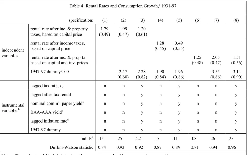
Interestingly, there is a positive correlation between consumption and capital rental rates both before and after 1947: the correlations are 0.57 and 0.44, respectively. Table 4 illustrates, since the estimates reported there are for samples extending back to 1931 – as far back as BEA data permit these calculations. The first column shows an estimated IES of 1.79, which is somewhat larger than the 1.10 estimate reported in Table 2 for the postwar period.

We see in Figure 3 how the after-tax rental rate is pretty similar before and after the war although, as discussed above, long run comparisons are sometimes sensitive to the measurement method. I therefore include a dummy variable for 1947-97 (divided by 100, so the coefficient is interpreted as growth rate percentage points) in the specification shown in Table 4's column (2). Consumption grows less after 1947 despite the (measure