Ambiguity Aversion and the Term
Structure of Interest Rates
Patrick Gagliardini, Paolo Porchia, Fabio Trojani
Editor:
Prof. Jörg Baumberger
University of St. Gallen
Department of Economics
Bodanstr. 1
CH-9000 St. Gallen
Phone
+41 71 224 22 41
Fax
+41 71 224 28 85
Email [email protected]
Publisher:
Department of Economics
University of St. Gallen
Bodanstrasse 8
CH-9000 St. Gallen
Phone
+41 71 224 23 25
Fax
+41 71 224 22 98
Ambiguity Aversion and the Term Structure of Interest Rates
Patrick Gagliardini, Paolo Porchia, Fabio Trojani
Author’s addresses:
Prof. Dr. Fabio Trojani
Institut für Banken und Finanzen
Universität St. Gallen
Rosenbergstrasse 52
9000 St. Gallen
Tel.
+41 71 224 70 74
Fax
+41 71 224 70 88
Email [email protected]
Website www.sbf.unisg.ch
Dr. Paolo Porchia
Prof. Dr. Patrick Gagliardini
Swiss Finance Institute
University of Lugano
Abstract
This paper studies the term structure implications of a simple structural economy in which
the representative agent displays ambiguity aversion, modeled by Multiple Priors Recursive
Utility. Bond excess returns reflect a premium for ambiguity, which is observationally distinct
from the risk premium of affine yield curve models. The ambiguity premium can be large
even in the simplest logutility model and is non zero also for stochastic factors that have a
zero risk premium. A calibrated low-dimensional two-factor economy with ambiguity is able
to reproduce the deviations from the expectations hypothesis documented in the literature,
without modifying in a substantial way the nonlinear mean reversion dynamics of the short
interest rate. In this economy, we do not find any apparent tradeoffs between fitting the first
and second moments of the yield curve and the large equity premium.
Keywords
General Equilibrium, Term Structure of Interest Rates, Ambiguity Aversion, Expec-
tations Hypothesis, Campbell-Shiller Regression.
JEL Classification
AMBIGUITY AVERSION AND THE TERM STRUCTURE
OF INTEREST RATES
Patrick Gagliardini
1Paolo Porchia
2Fabio Trojani
3This version: June 2007
First version: June 2004
41University of Lugano and Swiss Finance Institute, Via Buffi 13, CH-6900 Lugano, Switzerland. E-mail:
2Corresponding author. University of St. Gallen. Swiss Institute for Banking and Finance,
Rosen-bergstr. 52, CH-9000 St.Gallen, Switzerland. Phone: (41) 71 224 70 22. Fax: (41) 71 224 70 88. E-mail: [email protected].
3University of St. Gallen. Swiss Institute for Banking and Finance, Rosenbergstr. 52, CH-9000 St.Gallen,
Switzerland. Phone: (41) 71 224 70 50. Fax: (41) 71 224 70 88. E-mail: [email protected].
4We thank the Editor (Yacine A¨ıt-Sahalia) and two anonymous referees for many very valuable
sug-gestions. We are also grateful to Andrea Buraschi, Anna Cieslak, Tomas Bj¨ork, Domenico Cuoco, Jerome Detemple, Damir Filipovic, Peter Gruber, Alexei Jiltsov, Abraham Lioui, Pascal Maenhout, Alessandro Sbuelz and Andrea Vedolin for their useful comments. The authors gratefully acknowledge the financial support of the Swiss National Science Foundation (grants 12-65196/1, 101312-103781/1, 100012-105745/1 and NCCR FINRISK).
Introduction
This paper studies the term structure implications of a continuous-time production economy in which the representative agent displays ambiguity (Knightian uncertainty) aversion. First, we characterize the equilibrium in the structural economy with ambiguity aversion and identify the equilibrium market prices for risk and ambiguity. Second, we study the theoretical implications for the term structure of interest rates. Third, we calibrate a simple version of the model and study the extent to which ambiguity aversion can reproduce the empirical characteristics of the yield curve. Finally, we investigate how the degree of nonlinearity in the equilibrium short rate dynamics is affected by ambiguity aversion.
We extend the economy of Cox, Ingersoll, and Ross (1985) by assuming that the representa-tive investor does not know the form of the data generating process for the underlying production technology. This assumption introduces ambiguity into the economy and is based on a parsimo-nious one-parameter extension of the standard completely affine Cox, Ingersoll, and Ross (1985) term structure model. We specify investor’s aversion to ambiguity by a max-min expected utility optimization problem.1 Therefore, the excess return of any asset displays a separate premium for
ambiguity, which reflects the concern of the representative investor for a misspecification of the technology dynamics. The ambiguity premium can be substantial already for moderate levels of volatility and entails a nonlinear dependence on the underlying state variables.
A rapidly growing literature studies asset prices under ambiguity aversion in dynamic economies. Part of this literature tries to explain the equity premium and interest rate puzzles in a model with a plausible risk aversion parameter. Another part of this literature emphasizes the distinct portfolio behavior of ambiguity averse investors and the implications for option markets.2 However, none
of these papers studies the relation between ambiguity aversion and the term structure of interest rates. We introduce ambiguity aversion using the tractable setting of Anderson, Hansen, and Sargent 1See, among others, Gilboa and Schmeidler (1989), Epstein and Wang (1994), Epstein and Schneider (2003),
Anderson, Hansen, and Sargent (AHS, 1998, 2003).
2Uppal and Wang (2003) and Epstein and Miao (2003) show that ambiguity aversion can generate a home-bias
and under-diversification in the optimal portfolios of the investors in a two-countries economy. The equity premium and interest rate puzzles have been addressed, among others, in Chen and Epstein (2002), Maenhout (2004), Sbuelz and Trojani (2002) and Trojani and Vanini (2002). Leippold, Trojani and Vanini (2007) show that the combination of learning and ambiguity aversion additionally can explain the excess volatility puzzle. The limited stock market participation generated by ambiguity aversion in the absence of market frictions has been early emphasized by Dow and Werlang (1992). Cao, Wang, and Zhang (2004) and Trojani and Vanini (2004) study ambiguity aversion and endogenous limited stock market participation in a static and a dynamic setting, respectively. Liu, Pan, and Wang (2003) show that the ambiguity about the jump probability in the return of the underlying asset can mimic the typical ‘smirk’ shape of options’ implied volatilities.
(AHS, 1998, 2003) who measure ambiguity by a maximal constrained discrepancy between a set of likely misspecifications and a fixed reference belief.3 In this way, we can easily study the impact of
ambiguity aversion on the yield curve, in dependence of a single parameter that measures the degree of ambiguity in the economy. The preferences underlying the max-min expected utility problem solved by our representative agent are of the Recursive Multiple Prior Utility type, which implies a ‘rectangular’ set of relevant likelihoods, in the terminology introduced by Epstein and Schneider (2003), and admits an axiomatic foundation.
The term structure literature has documented several empirical regularities of US Treasury bond yields that are relevant for our work. In a reduced-form term structure setting, Duffee (2002) and Dai and Singleton (2002) emphasize the need for an essentially affine market price of risk specification which relaxes the restrictions of the completely affine models. This specification weakens the link between market price of risk and interest rate volatility for the Gaussian risk factors and improves the empirical predictability patterns for the bond excess returns. Cheridito, Filipovic and Kimmel (2005) further extend the completely affine specification of the market price of risk also for the volatility factors. In our model, a non–affine market price of risk relaxes the relation between bond excess returns and volatility. This market price of ambiguity is observationally distinct also from the market price of risk generated by yield curve models with state dependent risk aversion and/or money in the utility function, as in Buraschi and Jilsov (2005, 2007) and Wachter (2006).
Our main findings are as follows. First, in our specification of ambiguity aversion the market price of ambiguity has a non affine form. Therefore, the bond excess returns in our model cannot be obtained by any affine yield curve model or another model featuring second–order risk aversion. Moreover, stochastic factors that are not priced in the completely affine models pay an additional premium for ambiguity. Second, a simple two-factor calibrated economy with ambiguity aversion can reproduce the deviations from the expectations hypothesis documented in the empirical term structure literature. At the same time, it produces a reasonable volatility dynamics and a large equity premium. Third, the short rate dynamics implied by ambiguity aversion have similar persistence properties as those under the reference belief.4
The structure of the papers is as follows. Section I. presents the opportunity set of our ambiguity 3In their approach, the reference belief is interpreted as an approximate description of the unknown data generating
process. The discrepancy between models is measured by the relative entropy criterion.
4A¨ıt-Sahalia (1996, 1999) and Conley, Hansen, Luttmer, and Scheinkman (1997) provide empirical evidence for a
averse representative agent; it defines the set of relevant scenarios in the economy and introduces the max-min expected utility optimization that implies worst case optimal consumption and portfolio policies under ambiguity aversion. Section II. analyzes equilibrium interest rates, by characterizing the worst case solution in the max-min expected utility optimization, and derives the fundamental differential equation for bond prices. An example of a simplified two-factor economy in which the yield curve can be solved in closed form is also derived. Section III. calibrates a parsimonious extension of the Longstaff and Schwartz (1992) model with ambiguity aversion to bond yield data. It studies the implications of ambiguity aversion for the stylized facts of bond yields and addresses the issue of a potential nonlinearity in the short rate dynamics. Section IV. concludes. All proofs are in the Appendix.
I.
Model setting
The starting point of our analysis is the production economy framework developed by Cox, Ingersoll and Ross (1985). On an infinite time horizon, a probability space (Ω,F, P) endowed with the filtration (Ft)t≥0 supports a (k+ 1)−dimensional standard Brownian motion Z(t) =
[Z1(t), Z2(t), . . . , Zk+1(t)]0 that generates the uncertainty of the model. We call the probability
measureP the ‘reference belief’ of our production economy.
A.
Reference belief
We start deriving the implications of ambiguity aversion for a general form of the dynamics of the technology under the reference beliefP. Under the reference beliefP the basic constituents of the opportunity set available to agents are:5
1. A locally risk-less bond in zero net supply, with returnr.
2. A linear technology Qproducing a physical good that can be either reinvested or consumed. The output rate of the production technology is given by:
dQ
Q =α(Y)dt+σ(Y)dZ (1)
5All coefficients to appear are assumed to be continuously differentiable functions of the state variables.
Fur-thermore, we impose a uniform ellipticity condition on the matrix function ΞΞ0, where Ξ is the volatility matrix in
3. kfinancial assets, in zero net supply, that satisfy the stochastic differential equation
dS=ISβ(Y)dt+ISϑ(Y)dZ (2)
where S= [S1, S2, . . . , Sk]0 is the vector of price processes of these assets andIS denotes the
diagonal matrix diag[S1, S2, . . . , Sk].
4. kdriving state variablesY = [Y1, Y2, . . . , Yk]0 with dynamics
dY = Λ(Y)dt+ Ξ(Y)dZ (3)
The equilibrium in the economy is supported by a single representative agent with time preference rateδ≥0 and a logarithmic felicity function:6
U(c, t) =e−δtlog(c) ; c >0 .
To focus exclusively on the additional implications of ambiguity aversion for the yield curve, we have chosen a very standard structure of our economy under the reference belief; see Cox, Ingersoll and Ross (1985). In particular, an affine dynamics fordQ and dY implies an affine equilibrium yield curve.
B.
Model misspecification
The representative agent does not know the data generating process of the production technology. She considers a class of probabilistic scenarios, or contaminations, Ph around the reference belief.
These contaminations are interpreted as likely specifications for the technology dynamics and are assumed to be absolutely continuous with respect to the reference beliefP, as in AHS (1998, 2003). Therefore, contaminations of the reference belief are equivalently described by contaminating drift processes h. Since the scenarios Ph are mutually absolutely continuous, it follows that Z
h(t) = Z(t) +R0th(s)dsdefines a standard Brownian motion process underPh. Therefore, ambiguity takes
the form of a change of drift in the technology dynamics specified with respect to the reference belief. 6Gagliardini, Porchia and Trojani (2004) characterize the equilibrium with ambiguity aversion also in a finite
time-horizon economy with an ambiguity averse representative agent that features a CRRA utility over terminal wealth. The logarithmic setting is convenient to emphasize the main intuition concerning ambiguity aversion and the term structure of interest rates, while preserving a higher tractability.
Aversion to ambiguity arises by assuming that the representative agent is concerned with the worst case scenario in a neighborhood of the reference belief. In order to identify such a neighbor-hood, we assume that the contaminating drift processeshsatisfy the following upper bound:
h0h≤2η (4)
whereη≥0 is a fixed parameter. For tractability, we restrict our treatment to the class of Markov Girsanov kernels h(Y) defined by measurable functions h(·). H denotes the class of admissible Markovian drift contaminations satisfying the bound (4). This family of admissible drift contamina-tions admits a clear interpretation in terms of a maximal allowed statistical discrepancy betweenPh
andP; see AHS (1998, 2003). Precisely, it implies a maximal boundηon the instantaneous growth rate of the relative entropy between any admissible contaminated modelPh and the reference belief P. It follows that we can interpretηas a measure of the degree of ambiguity in the economy: Larger values of η imply a higher ambiguity. Moreover, forη →0 we obtain the standard Cox, Ingersoll and Ross (1985) economy. Note that the bound (4) constrains the instantaneous time-variation of the relative entropy between these two models, not just its global continuation value. Therefore, our specification of ambiguity aversion is based on a rectangular set of priors, using the terminology of Epstein and Schneider (2003), which implies a dynamically consistent preference ordering supported by Multiple Priors Recursive Utility.7
C.
Max-min expected utility
The representative agent finances her consumption process c(t) by trading continuously in the financial assets at the equilibrium prices. If we denote by Σ the (k+ 1)×(k+ 1) diffusion matrix of the available opportunity set,
Σ(Y) = σ(Y) ϑ(Y) 1×(k+1) k×(k+1) (5)
then the usual dynamic budget constraint, coupled with the appropriate integrability conditions,8
7See also Trojani and Vanini (2004), p. 289, for a more detailed discussion. 8An admissible trading strategyπ= [ω v]0is such that:
Zt
0
|ω(s)(α(s)−r(s))|+|v(s)(β(s)−1kr(s))|+|π(s)0Σ(s)h(s)|+π(s)0Σ(s)Σ(s)0π(s)2ds <∞ (6) P-a.s. for everyt >0.
implies feasibility of consumption plans: dW(t) W(t) = · ω(t) (α(t)−r(t)) +v(t)¡β(t)−r(t)1k ¢ + µ r(t)− c(t) W(t) ¶¸ dt +π0(t) Σ(t) [dZ(t) +h(t)dt] (7)
whereπ= [ω 1×vk]0 ∈Rk+1 contains the portfolio weights ω andv0 invested in the technology and the financial assets, respectively, 1k is a k−dimensional vector of ones and W(t) is the financial
wealth of the representative agent at timet. In order to prevent arbitrage opportunities, we follow Dybvig and Huang (1988) and assume that W(t) ≥ 0 for every t ≥ 0. The ambiguity averse representative investor solves the max-min expected utility program
J(x, y) = sup c , π hinf∈HE h ·Z ∞ 0 e−δslog(c(s) )ds ¸ (8) s.t. (7)
where W(0) =x, Y(0) =y andEh[·] denotes expectations under measure Ph. In a Cox, Ingersoll
and Ross (1985) economy, financial securities are in zero net supply. Therefore, their expected returns are shadow prices for the constraint to hold a null portfolio weight on these securities. We have the following definition of equilibrium.
Definition 1. Anequilibriumis a vector (c∗, h∗, r∗, β∗) of a consumption policy, a model contami-nation, interest rate and financial assets return processes, such that:
1) The equilibrium consumption policy c∗ and the drift contaminationh∗ are optimal according to the following preference ordering representation:
inf h∈HE h ·Z ∞ 0 e−δslog(c(s) )ds ¸ . (9)
2) Optimal consumption is financed by a trading strategy according to which wealth is totally invested in the technology:
II.
Characterization of equilibrium and pricing
This section studies the equilibrium in the production economy with ambiguity aversion and the resulting implications for the yield curve.
A.
Equilibrium value function
In equilibrium, the value function (8) is evaluated at the market-clearing values of the short interest rate and the returns on financial assets. This value function depends on both the model selection in the corresponding max–min expected utility problem and the optimality conditions evaluated at equilibrium prices. We can postpone the selection of the optimal contaminating drift
h∗ to the determination of the dependence of the interest rate and the excess returns of financial assets on any admissible contaminating drift h ∈ H. Therefore, we interchange the order of the maximization and the minimization in problem (8) and observe that the resulting innermost program is a standard optimization, in which the equilibrium conditions are easily handled by standard methods.9 The following Proposition exploits this fact to characterize the optimal contaminating
drifth∗ in our economy.
Proposition 1 In equilibrium, the value function of the ambiguity averse representative investor is given by J(x, y) =−1 δ+ log(δx) δ +V(y) (11) where V(y) = inf h∈HE h ·Z ∞ 0 e−δt Z t 0 µ α(s)−1 2σ(s)σ(s) 0+σ(s)h(s) ¶ ds dt ¸ (12) subject to dY = Λ(Y)dt+ Ξ(Y) (dZ+hdt) .
The equilibrium contaminating drift that solves the model selection problem in the max-min opti-mization (8) is given by h∗=−p2η Ξ 0V Y +σ0 q (Ξ0VY +σ0)0(Ξ0VY +σ0) (13) 9See Appendix A for a formal justification of this step.
where VY denotes the gradient of V with respect to the state variables Y. The value function V solves the following Hamilton-Jacobi-Bellman (HJB) equation
V0 YΛ + 1 2trace [Ξ 0V Y YΞ]− p 2η q (Ξ0VY +σ0)0(Ξ0VY +σ0) +α−1 2σσ 0−δV = 0 (14)
whereVY Y is the Hessian matrix of V with respect to the state variable Y.
The value functionJ of the ambiguity averse representative investor depends on value function V, which solves the HJB equation (14). In the definition of V, the contaminating drifth affects the state variables dynamics by shifting probabilities over the space of sample paths in an absolutely continuous fashion. The expectation inside equation (12) is defined over a discounted “running cost”
e−δtl(t), say, where: l(t) = Z t 0 µ α(s)−1 2σ(s)σ(s) 0+σ(s)h(s) ¶ ds . (15)
The difference of the first two terms in this integral reflects the impact of the standard risk-return tradeoff on the indirect utility of a representative agent with logarithmic utility function in a Cox Ingersoll and Ross (1985) production economy. This difference depends on the varianceσ(s)σ0(s) of the production technology. Therefore, it affects the indirect utility of the representative agent by means of the well-known second-order risk aversion effect. The third term in the integral (15) is proportional to the volatility of the production technology, weighted by the contaminating drifth. If the optimal controlh∗is constant, the contribution of this term is proportional toσ(s) and impacts on the indirect utility of the representative agent in a way that is observationally equivalent to a first–order risk aversion effect. It is easy to show that this feature arises in our economy when the admissible drift-contaminations h∈ H are one-dimensional. For a general multi-factor technology with stochastic volatility, the optimal worst case drift contamination is state-dependent. In this case, ambiguity aversion impacts on the indirect utility of the representative agent in a way that is different from the effect of both first– and second–order risk aversion.10
10Ambiguity aversion effects similar to second–order risk aversion are precluded when the volatility of the production
technology is stochastic, because the bound (4) implies a constant squared norm of the optimal drift contamination
B.
Equilibrium interest rate and market price of ambiguity
The equilibrium interest rate and the market prices of risk and ambiguity follow as a direct Corollary to Proposition 1.
Corollary 1 The market price of risk and ambiguity in the economy with ambiguity aversion is given by λ=σ0+p2η Ξ 0V Y +σ0 q (Ξ0V Y +σ0)0(Ξ0VY +σ0) =:λR+λA (16)
and the equilibrium interest rate is:
r=α−σλ . (17)
The market price of risk and ambiguity is the sum of the market price of risk λR = σ0 and the
market price of ambiguity
λA= p 2η Ξ 0V Y +σ0 p (Ξ0VY +σ0)0(Ξ0VY +σ0) . (18)
λRtakes the standard completely affine form, in which risk compensation per unit of risk is identical
to the volatility of the production technology. Without ambiguity (η = 0), this feature implies a strong relation between excess returns and the volatility of financial assets in the economy, which is at odds with the stylized facts of the US Treasury yields. Duffee (2002) and Dai and Singleton (2002) emphasize the need of a more flexible market price of risk specification, linked to factors that might affect the slope of the yield curve, in addition to the volatility. To this end, Duffee (2002) proposes the essentially affine specification of the market price of risk, which breaks the link between the market price of risk and the volatility of Gaussian factors. With the same purpose, Cheridito, Filipovic and Kimmel (2005) have further extended the market price of risk specification for the stochastic volatility factors in reduced–form models. In our model, the market price of ambiguity
λA breaks the connection between excess returns and volatility, but its nonlinear form implies a
yield curve that is not affine. λAdepends on Ξ, the volatility matrix of all state variables, and the
marginal utility VY of the representative investor with respect to the state variables. This is the
reason why bonds excess returns can be associated to other state variables than volatility. Moreover, the components of the product Ξ0V
take both positive and negative values, consistently with the empirical evidence. The dependence of the market price of ambiguity on the term Ξ0V
Y is due to the non-myopic
portfolio behavior of the ambiguity averse representative agent, even with logarithmic utility. In-tuitively, the representative investor hedges her portfolio against future changes in the worst case opportunity set, which are in a one-to-one relation to the realizations of the worst case drift distor-tion h∗. This hedging motive is different from the standard hedging motive against the risk of a change in the opportunity set, as perceived under the reference belief, which is well-known to vanish for log-utility investors. It follows that state variables uncorrelated with the technology process can pay a premium for ambiguity, even if their risk would not be priced in a standard Cox, Ingersoll and Ross (1985) economy.
C.
Term structure of interest rates
Given the expression for the market price of risk and ambiguity in Corollary 1, we can now price any interest rate derivative by standard arbitrage arguments. The change of driftφY from the
reference beliefP to the risk neutral probability measureQis given by:
φY = Ξλ= Ξ σ0+p2η q Ξ0VY +σ0 (Ξ0V Y +σ0)0(Ξ0VY +σ0) (19)
where the value functionV solves the HBJ equation (14). Given the drift change φY, the price of
a contingent claim with maturityT and paying off at a rate Ψ(Y, t), t≤T, is characterized by the following fundamental partial differential equation.
Proposition 2 The price at time t, F(Y, t), of a contingent claim with instantaneous pay-off
Ψ (Y, t),t≤T, satisfies the partial differential equation:
1 2trace µ Ξ Ξ0 ∂ 2F ∂Y ∂Y0 ¶ + (Λ−φY) 0∂F ∂Y −r F + ∂F ∂t =−Ψ (20)
with boundary conditionF(Y, T) = Ψ (Y, T), whereris the equilibrium short rate given in Corollary 1 andφY is the risk neutral drift change defined in equation (19).
Compared to the completely affine setting, ambiguity aversion alters the fundamental pricing equa-tion through the different equilibrium interest rate r and the corresponding change of drift φY.
Therefore, the Feynman–Kac theorem gives the usual probabilistic representation of the derivative price: F(Y, t) =EQ " Z T t e−Rs t r(u)duΨ(Y(s), s)ds+e− RT t r(s)dsΨ (Y(T), T) ¯ ¯ ¯ ¯ ¯Ft # (21) whereEQ[·] denotes the expectation with respect to the risk neutral probability measureQunder
ambiguity aversion. A major difference with respect to the pricing problem of a completely affine Cox, Ingersoll and Ross (1985) economy emerges, because the equilibrium interest rate r and the drift changeφY are preference-dependent parameters when ambiguity aversion is present. They are
determined by the value function gradientVY appearing in the formulas of Corollary 1. Therefore,
the pricing problem cannot be separated from the equilibrium computation of the market price of ambiguityλA in equation (18). As a consequence, in the economy with ambiguity aversion we have
to solve the system of partial differential equations (14) and (20) in order to compute the equilibrium yield curve.11
D.
Closed form solutions in a simple model setting
We first discuss a simplified two-factor economy in which the representative investor exhibits ambiguity only over one of the state variables driving the reference belief. This assumption implies a more restrictive form of the ambiguity premium, but yields closed-form expressions for the term structure of interest rates. Therefore, this model provides a basic intuition for the role of ambiguity aversion in the yield curve context. It addition, it clarifies the limitations of an economy in which the structure of ambiguity is independent across the relevant state variables. A more general economy in which ambiguity aversion affects the subjective dynamics of all states variables is analyzed in Section III., where we calibrate the model to US Treasury yields data.
i) Technology process
The reference belief dynamics of the production technology satisfies a two-factor Longstaff and Schwartz (1992) model. Therefore, under any model contaminationPh, the production technology
11These equations can be solved in closed form only for particular model settings, e.g., by assuming a Gaussian
state variables dynamics forY or by introducing additional restrictions on the structure of the optimal drift distortion
dynamics can be written as: dQ Q = (g1Y1+g2Y2)dt+l p Y2 ³p 1−ρ2(dZ 1+h1dt) +ρ(dZ3+h3dt) ´ (22) dY1 = (a1+m1Y1)dt+n1 p Y1(dZ2+h2dt) (23) dY2 = (a2+m2Y2)dt+n2 p Y2(dZ3+h3dt) (24)
whereZ = [Z1, Z2, Z3]0is a three dimensional standard Brownian motion, andgi, ai, mi, ni,i= 1,2,
and l are scalar parameters. In this model, the instantaneous correlation between dQ/Q and dY1
is zero, but the correlation betweendQ/Q and dY2 is allowed to be nonzero, and is given by the
parameter ρ. It follows that the variance of the technology return is the only state variable, in addition to the technology itself, which pays a non-zero risk premium in this economy. For illustration purposes and for analytical tractability, we make the following assumption, which implies that the representative investor perceives ambiguity only about the shocks in the dynamics of the conditional variance of the technology.
Assumption 1 The admissible contaminating drift process h = (h1, h2, h3)0 is restricted to be of
the formh= (0,0, h3)0. Moreover, the parameter constrainta2=n22/4 holds.
The parameter constraint ona2 in Assumption 1 allows us to obtain closed form solutions for the
term structure of interest rates.
ii) Ambiguity premium
Under Assumption 1, it is easy to show from Proposition 1 that the optimal contaminating drift ish∗ = (0,0,−√2η)0. The market price of risk and ambiguity vector is then immediately inferred from Corollary 1: λ=lpY2 p 1−ρ2 0 ρ | {z } λR +p2η 0 0 1 | {z } λA . (25)
The market price of risk λR is completely affine, since it is proportional to the volatility of the
production technology. The market price of ambiguityλAis constant and loads only on the Brownian
ambiguity aversion does not impact on the other shocks in the economy. It follows that even when the market price of risk for the shockdZ3 in the technology volatility is zero (ρ= 0), the market
price of ambiguity for these shocks is positive. Moreover, the market price of ambiguity does not vanish when the production technology risk vanishes (Y2 ↓ 0). Therefore, ambiguity premia tend
to dominate risk premia in determining excess returns precisely when the aggregate risk in the economy is low. The observationally different form of the market price of ambiguityλAfollows from
our specification of ambiguity aversion in the max-min problem (8), which gives rise to an inherently different economic behavior than the one generated by the standard risk aversion. Standard risk aversion behavior in the Cox, Ingersoll and Ross (1985) economy implies a concern for variance– covariance risk, i.e., second–order risk aversion, which generates equilibrium expected excess returns that are proportional to variances and covariances of the risk factors. In contrast, our model of ambiguity aversion generates a concern for small risks that does not fit into this framework.12
iii) Term structure and bond excess returns
Under Assumption 1, a remarkable feature of the Longstaff and Schwartz (1992) economy with ambiguity is that the differential equations (14) and (20) needed to compute the yield curve are both solvable in closed form. The priceP(t, T) of a zero bond of maturityT is given by:
P(t, T) = exp ³ A(t, T, η) +B(t, T)Y2+ p 2ηC(t, T)pY2+D(t, T)Y1 ´ (26)
with functions B(t, T), C(t, T) and D(t, T) admitting closed form expressions.13 The nonlinear
dependence of logP(t, T) on the state variableY2emphasizes the non-affine structure of the model.
Using the explicit expression for the change of driftφY in equation (19):
φY = Ξλ= 0 √ Y1 0 0 0 √Y2 lp1−ρ2√Y 2 0 lρ√Y2+ √ 2η = 0 lρY2+ √ 2ηY2 (27)
12Not all specifications of ambiguity aversion in the literature are observationally distinct from second–order risk
aversion behavior. Maenhout (2004), e.g., models ambiguity aversion by a tilted robust control problem that is observationally equivalent to second–order risk aversion. For a setting with logarithmic utility, also the penalized control problem in AHS (1998, 2003) delivers a model of ambiguity aversion that is observationally equivalent to second–order risk aversion behavior. Trojani and Vanini (2004) provide a detailed discussion of the observational distinctions of different models of ambiguity aversion.
we can also easily compute the instantaneous expected excess return on the zero bond: 1 dtEt · dP(t, T) P(t, T) ¸ −r = PY(t, T) P(t, T) φY = µ B(t, T) +C(t, T) 2 r 2η Y2 ¶ ³ lρY2+ p 2ηY2 ´ = lρB(t, T)Y2+ p 2η µ B(t, T) +lρC(t, T) 2 ¶ p Y2+ηC(t, T) (28)
wherePY(t, T) denotes the gradient of the zero coupon price with respect to the state variables. It
follows that whenη >0 the excess returns on bonds are non affine functions of the state variableY2.
This simple extension of the affine economy implies a richer behavior of the term structure of bond excess returns, especially for states of moderate volatility risk. More generally, when Assumption 1 is not satisfied, bond excess returns are non affine functions of all state variables in the model. This additional flexibility of the model is potentially useful for explaining the stylized facts of bond returns. Empirical research has accumulated substantial evidence that bond excess returns are predictable by term structure variables, such as the term structure slope, the spot-forward spread, or a linear combination of forward rates (Fama and Bliss, 1987, Campbell and Shiller, 1991, and Cochrane and Piazzesi, 2005). In the next section, we investigate if ambiguity aversion can help explain this empirical evidence within a simple low-dimensional two-factor Longstaff and Schwartz (1992) economy.
III.
Model calibration and empirical analysis
We calibrate a two-factor Longstaff and Schwartz (1992) model with ambiguity aversion to US Treasury yields data and investigate the empirical yield curve implications of our setting. Using a low–dimensional two–factor dynamics to explain the yield curve stylized facts is a difficult task. Dai and Singleton (2003), e.g., show that three-factor essentially affine models have difficulties in matching at the same time the first and the second moments of yields. In particular, a completely affine model with a three–factor CIR dynamics fails completely in fitting the predictability of bond returns. Therefore, we show that our one-parameter extension of the affine model class can help in reproducing some of these stylized facts.
h ∈ H, defined by the bound (4), is given in equations (22)-(24) without imposing Assumption 1. In contrast to the model presented in Section II. D., the current specification does not admit closed-form value function and yield curve solutions for the differential equations (14) and (20).
A.
Calibration of the model
We calibrate our model using interest rate data for the sample period between January 1960 and December 2000. The interest rate data from January 1960 to February 1991 are obtained from the McCulloch (1990) and Kwon (1992) data-set, which was extended with the methodology described in Buraschi and Jiltsov (2007) until December 2000.14 The fact that both solutions of the
differential equations (14) and (20) are not given in closed-form makes the calibration of the Longstaff and Schwartz (1992) model with ambiguity aversion a challenging task. A completely numerical calibration approach is very computationally demanding. Moreover, calibrated parameters of such a procedure can suffer from an inherent instability, because the objective function minimized by the calibration procedure depends itself on the solution (14) of another optimization problem. This feature implies a potentially non-smooth optimization problem, in which one numerical optimization is embedded in another one. We circumvent this problem by a simple analytical approximation, which exploits the fact that the ambiguity parameterη is typically a small number for application purposes.15
i) Yield curve asymptotics
We first assume that the gradient of the value function in equation (14) can be approximated by a straightforward zero–order expansion:
VY(Y) =V0Y(Y) +O(√η) (29)
where V0Y is the gradient of the zero–order value function in the Longstaff and Schwartz (1992)
economy with no ambiguity (η= 0). This gradient is known in closed-form.16 Inserting the
expan-sion (29) in equation (16), the following first-order approximation for the market price of risk and 14We thank Andrea Buraschi and Alexei Jiltsov for providing the dataset.
15The numerical value ofηimplied by all our calibrations is always less than 0.0136. 16The explicit expression forV(Y) is:
V(Y) =K1Y1+K2Y2+K3 (30)
ambiguityλholds:17 λ=σ0+p2η Ξ 0V 0Y +σ0 p (Ξ0V 0Y +σ0)0(Ξ0V0Y +σ0) +o(√η) . (31)
Using this approximation, similar first–order expansions for the equilibrium interest raterand the change of driftφY follow from equations (17) and (19). By inserting these approximations in the
fundamental pricing equation (20), we finally obtain a first–order expansion for the yield curve under ambiguity aversion. This expansion depends only on the zero–order value function gradient
V0Y and the zero–order yield curve (η = 0) in the Longstaff and Schwartz (1992) economy, which
are both known in closed form. In this way, we can completely avoid a numerical solution of the optimization problem (12) when computing the yield curve under ambiguity aversion. The first– order approximation of the yield curve under ambiguity aversion is provided in the next Proposition. Proposition 3 Let R(t, T) =− 1
T−tlogP(t, T) be the zero coupon bond spot rate for maturityT. Then, the following first–order expansion holds:
R(t, T) =R0(t, T)− p 2η P1(t, T) (T−t)P0(t, T)+o( √ η) (32)
where R0 and P0 are the closed-form spot rate and zero coupon bond price in the Longstaff and
Schwartz (1992) economy without ambiguity (η = 0). The first–order termP1(t, T)is given by:
P1(t, T) =EQ0 "Z T t exp µ − Z s t (α(u)−σ(u)σ0(u))du ¶ Ψ0(Y(s), s−t)ds # (33)
whereQ0 is the risk neutral probability in the Longstaff and Schwartz (1992) economy without
am-biguity, which is associated with the risk neutral drift changeφ0Y = Ξσ0. The payoff functionΨ0 in
equation (33) is defined for t≤s≤T by:
Ψ0(Y, s−t) =−(Ξ
0V
0Y +σ0)0[(s−t)Ξ0R0Y(t, s) +σ0]
p
(Ξ0V0Y +σ0)0(Ξ0V0Y +σ0) P0(t, s) (34)
whereR0Y(t, s)is the gradient ofR0(t, s)with respect to the state variable Y.
Using Proposition 3, we easily obtain accurate first–order approximations forR(t, T), by computing 17The higher order of the error in the approximation forλ, relative to the expansion (29), comes directly from the
fact that the market prices of risk and ambiguity depends on the gradientVY through a term that is pre-multiplied by√η.
the expectation (33) with Monte Carlo methods. Since all terms defining Ψ0 in equation (34) are
known in closed form for the Longstaff and Schwartz (1992) economy without ambiguity, this task can be accomplished quite efficiently.
ii) Calibration results
Whenη >0, we use the first–order yield curve approximation:
R(t, T)≈R0(t, T)−
p
2η P1(t, T)
(T−t)P0(t, T) (35)
to calibrate our model to the US Treasury yields data. Whenη= 0, we use the well–known closed form expression R0(t, T) for the Longstaff and Schwartz (1992) economy without ambiguity. We
calibrate the model to the unconditional mean and volatility of the one-month and the one-year yields, as well as to the first–order autocorrelations and the contemporaneous covariance of these yields. In order to provide additional information on the predictability structure in our interest rate data, we also match the Campbell and Shiller (1991) regression coefficients of two regressions of 10–year and 2–year yield changes on the past term structure slope, as measured with respect to the 6–month yield; see Section III. B. for more details.
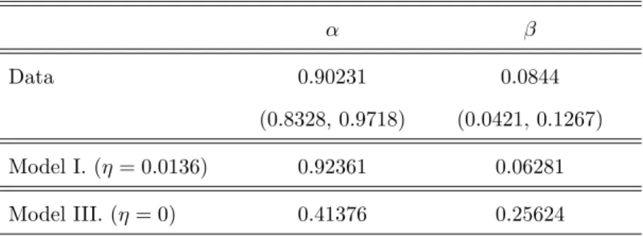
Table I summarizes the set of moment conditions used and the calibration results obtained for three distinct model settings. Setting I. is based on an unconstrained calibration of the ambiguity parameterη. Setting II. constrains the ambiguity parameter to an intermediate value between 0 and the unconstrained calibrated value obtained for setting I. Setting III. constrains the ambiguity parameter to 0, as in the standard Longstaff and Schwartz (1992) economy.
Insert Table I about here.
The optimal ambiguity parameter calibrated for Setting I. isη= 0.0136. The calibration results for the unconstrained model are quite good, with largest percentage errors of approximately 10% on the calibrated moments. Larger calibration errors are obtained in the other settings for the calibrated Campbell and Shiller (1991) regression coefficients and for the calibrated covariance between one-month and one-year yields. The poor performance in calibrating the Campbell and Shiller (1991) coefficients for settings in whichη≈0 is consistent with the inability of completely affine models to match the empirical bond predictability patterns. However, the results in Table I. highlight that a small perturbation of the completely affine Longstaff and Schwartz (1992) economy can ameliorate
substantially the empirical fit when ambiguity aversion is explicitly addressed in the definition of the model.
Using the calibrated parameters, we can also study the quality of the first–order yield curve approximation (32) for the ambiguity parameterη = 0.0136 implied by our unconstrained setting. We compute numerically the yield curve for several conditioning values of the state variablesY1and
Y2, by solving numerically equations (14) and (20) at the calibrated model parameters. We then
compare the yield curve with the one implied by the approximation (32). We find that our simple first–order approximation is quite accurate, even for longer maturities, with relative approximation errors typically below 10%. Figure I illustrates the quality of our yield curve approximation for three different yield curve states.
Insert Figure I about here.
The next section produces additional empirical evidence that our first–order yield curve approx-imation with ambiguity aversion improves the description of the salient features of Treasury yield data implied by affine models.
B.
Empirical findings
We study the goodness-of-fit of the Longstaff and Schwartz (1992) yield curve model with ambi-guity aversion with respect to some well–known stylized facts of US Treasury yields data.
i) Deviations from the expectations hypothesis: Campbell–Shiller Regressions
The expectations hypothesis of interest rates implies that bond returns are unpredictable. This hypothesis can be tested by a Campbell and Shiller (1991) time series regression of yield changes on the slope of the term structure:
R(t+m, t+n−m)−R(t, t+n) =β0+β1 m
n−m[R(t, t+n)−R(t, t+m)] +εt (36)
where nis the maturity of the zero bond and mis the length of the time period over which bond returns are measured. We fixn= 1,2,3,5,7,10 years to maturity andmto be 6 months. Table II presents the coefficient estimates implied by our data set, together with those obtained for a long simulated sample of 5000 observations from the calibrated models I., II. and III. introduced in the
last section. The coefficients for the 2–years and 10–year times to maturity, which have been used to calibrate the models, have been underlined.
Insert Table II about here.
The first panel of Table II emphasizes the way in which the expectations hypothesis is violated in the data. The estimated slope coefficients in these regressions are all significantly different from one: They are all negative and their absolute value increases with maturity. The last panel of Table II highlights the failure of the completely affine models to mimic the violations of the expectations hypothesis in the data: All estimated coefficients are positive and fall outside the confidence intervals estimated with our data set. The second panel of Table II shows that the model with an uncon-strained calibrated ambiguity parameter can fit well the patterns of the estimated slope coefficients in the data: all estimated coefficients are negative and fall inside the confidence intervals estimated with our data set. The model with the constrained ambiguity parameterη = 0.005 also delivers negative estimated slope coefficients. However, in about half of the cases these estimates are outside the confidence intervals from the data.
These findings indicate that in the Longstaff and Schwartz (1992) economy ambiguity aversion can produce the predictability of bond excess returns consistent with the data. The distinct pre-dictability patterns of the completely affine versus the ambiguity averse version of the model are generated by the very different equilibrium excess returns implied by these two models. In both models, the market price of risk has a very simple structure, which is independent of the first state variable Y1. However, in the model with ambiguity aversion the ambiguity premium additionally
influences excess returns in a nonlinear way. If follows that the ambiguity premium is not affine, depends on both state variablesY1 andY2 and implies excess returns that can be both positive and
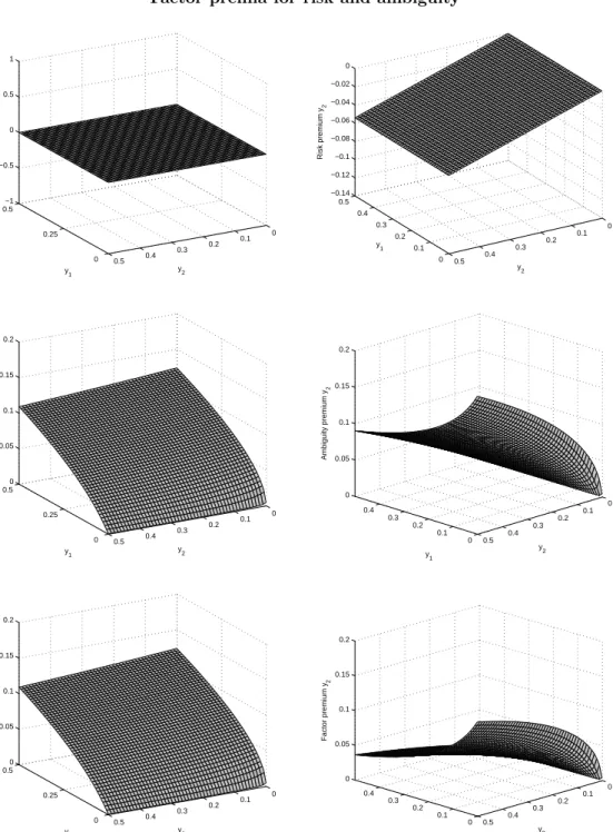
negative, in dependence of the realized state of the economy. Figure II plots the instantaneous risk and ambiguity premia ΞλR and ΞλA forY1 andY2, as a function of the relevant state (Y1, Y2) of
the economy.
Insert Figure II about here.
The risk premium for the stateY1is always zero. The one for the stateY2is negative, independent
of Y1 and decreasing in Y2. The negative risk premium for Y2 is due to the negative correlation
parameterρ between dQ/Q and dY2 implied by the calibrated model. The ambiguity premia for
ambiguity premium forY1is increasing inY1and almost independent ofY2. The ambiguity premium
forY2 is increasing inY2 and decreasing inY1.
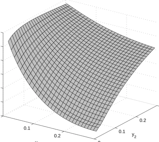
These features generate the more flexible structure of bond excess returns, which can accom-modate the violations of the expectations hypothesis. To illustrate this point, Figure III plots the instantaneous expected excess return
Et µ dP(t, t+τ) P(t, t+τ) ¶ −r=PY(t, t+τ) P(t, t+τ) φY
of a 5 year–maturity bond, as a function of the relevant state (Y1, Y2).
Insert Figure III about here.
The expected excess return is positive for a large set of possible states, it is increasing inY2 and
decreasing in Y1. Consistently with the empirical evidence, it can become negative for moderate
values of Y2 as the state Y1 increases. Therefore, the model can generate predictability patterns
driven by the two-dimensional system of state variables (Y1, Y2). In the two–factor Longstaff and
Schwartz (1992) economy, this feature implies that the slope of the yield curve is a predictive factor for future bond returns.
ii) Short interest rate dynamics
In the Longstaff and Schwartz (1992) economy with ambiguity aversion, the market price of ambiguity influences in a direct way the level of the short rate, by modifying the instantaneous excess return on the production technology, which is a non-affine function of the state variables. Therefore, it is interesting to study the properties of the short rate dynamics under ambiguity aversion, and to compare them with those of the completely affine model withη = 0.
A useful tool to study these features is the pull function – see Conley, Hansen, Luttmer, and Scheinkman (1997) – which is a measure of the conditional speed of mean reversion for nonlinear diffusion processes.18 The pull function P(r?) of the nonlinear diffusion process r(t) is defined
through the conditional probability thatr(t) reaches the valuer?+² beforer?−², if initialized at r(0) =r?, when²is small. To first–order in², this probability is given by:
1 2+² µr(r?) 2σ2 r(r?) +o(²), (37)
18A different approach to study the properties of nonlinear diffusion processes has been proposed by A¨ıt-Sahalia
whereµrandσrare the drift and diffusion functions of the short rate diffusion process, and the pull function is defined by P(r?) = µr(r?) 2σ2 r(r?) . (38)
We reproduce the pull function of the calibrated models with and without ambiguity by estimating it on a long sample of 25000 simulated data from these models. The pull function is estimated with the semi-nonparametric method in Conley, Hansen, Luttmer and Scheinkman (1997) for a flexible specification of the drift and the local volatility of the short rate; see Appendix C for details.19
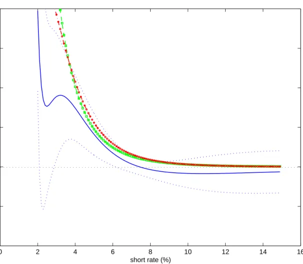
Figure IV presents the pull functions estimated for the short rate processes of the calibrated models with and without ambiguity (forη = 0.0136 andη = 0, respectively). For comparison, we also plot the empirical pull function and a 95% confidence interval around it, estimated using our data set.
Insert Figure IV about here.
The pull function of the short rate process with ambiguity aversion is very similar to the one of the short rate in the calibrated two-factor completely affine Longstaff and Schwartz (1992) model. Both pull functions highlight a pronounced nonlinearity of the mean reversion speed of the short rate in the calibrated models. The nonlinearity of the mean reversion obtained for the completely affine two-factor setting at the calibrated parameters is substantial. As shown in Buraschi and Jiltsov (2007), this feature could not have been generated, e.g., by calibrating a single-factor Cox, Ingersoll and Ross (1985)–type short rate process, in which the pull function is explicitly given by:
P(r?) = λ(r−r?)
2σ2r? (39)
for some positive constantsλ, σandr. Over a good spectrum of short interest rate values, the pull functions of the calibrated models are contained in the 95% confidence interval around the empirical pull function. For short rate levels less than 4%, the model pull functions are outside the (large) confidence intervals. For these interest rate levels, however, it is possible that the point estimates and the estimated confidence intervals are not very reliable, due to the low fraction of short rate ob-19The structural dynamics of the short interest rate implied by our two–factor model is not autonomous. Like in
indirect inference estimation, the semi-nonparametric model defining the pull function estimates can be interpreted as a flexible auxiliary model for the short rate diffusion process.
servations below 4% in our data set. Overall, these findings indicate that the Longstaff and Schwartz (1992) model with ambiguity aversion can reproduce the empirical failures of the expectations hy-pothesis without modifying in a substantial way the short rate nonlinear mean reversion features of the completely affine version of the model.
iii) Additional features
The affine term structure literature documents the difficulties of low-dimensional affine factor models to match the dynamics of both the first and second moments of yields. Dai and Singleton (2003), e.g., find that an A2(3) essentially affine model with one CIR and two Gaussian factors
produces a conditional volatility that is approximately consistent with the data. However, this model fails largely in explaining the conditional first moments of bond yields. AnA1(3) essentially
affine model with two CIR volatility factors and one Gaussian factor matches even worse the volatility dynamics.
Is the time variation of the second moments in the calibrated model with ambiguity aversion roughly consistent with the empirical evidence? To investigate this issue we perform a simple exercise as in Dai and Singleton (2003), and estimate a GARCH(1,1) model for the 5-year yield, using both our yield data and a large sample of 5000 observations simulated at the calibrated model parameters.20 The results of this exercise are summarized in Table III.
Insert Figure Table III about here.
In the calibrated model I., a moderate ambiguity (η = 0.0136) yields estimates of the GARCH parameters that are well within the 95%–confidence intervals around the GARCH point estimates in the data. The GARCH estimates for the calibrated Longstaff and Schwartz (1992) model III. (η= 0) are, instead, at odds with those estimated in the data. The completely affine model implies tight restrictions between bond excess returns and their volatility. The consequence of this feature is that the calibrated Longstaff and Schwartz (1992) model III. cannot match simultaneously the Campbell-Shiller (1991) regression coefficients and the volatility of interest rates. On the top of the unsuccessful attempt to match the Campbell-Shiller (1991) regression coefficients in our calibration, the model fails with respect to the yield volatility dynamics. The model with ambiguity aversion breaks the link
between bond excess returns and yield volatility. In this way, it can generate reasonable predictability and volatility patterns.
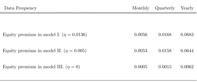
To conclude our empirical analysis, we study the equity premium implied by our calibrated yield curve model with ambiguity aversion. Asset pricing models with time separable preferences find it hard to match both the observed equity and bond premia, because of the strong link they imply between excess returns and the intertemporal elasticity of substitution (IES). For realistic risk aversion parameters, the observed equity premium is too high and the model implied bond excess returns are too low, in comparison to their volatility. The ambiguity premium in our model detaches excess returns from the elasticity of intertemporal substitution. The calibrated market price of ambiguity allows us to accommodate the empirical predictability patterns of US Treasury yields. The IES of one allows us to match well the moderate volatility of bond yields.21 Can the
model match the large historical equity premium as well? To answer this question, we simulate the model implied unconditional equity premium for the investment in the production technology, evaluated at the calibrated model parameters. Table IV summarizes our findings.
Insert Table IV about here.
As expected, the equity premium in the completely affine economy is very small and amounts to about 0.6% at an annual frequency. The equity premium of the unconstrained economy with ambiguity aversion is much larger and is about 6.8% on an annual basis.
IV.
Conclusions
We extend structural continuous-time yield curve models to incorporate ambiguity (Knightian uncertainty) aversion, modeled by Multiple Priors Recursive Utility. This extension is parsimonious in the sense that it is parameterized by a single additional parameter: The degree of ambiguity in the economy. When the representative investor displays aversion to ambiguity, the excess returns on bonds reflect also a premium for ambiguity, which is observationally distinct from the premium they pay for risk. Even in the simplest log-utility economy, the ambiguity premium can be large. Moreover, it is nonzero also for state variables that do not pay a premium for risk. We show that these features have non trivial implications for the model’s ability to fit some stylized yield curve
facts. We calibrate to US Treasury yields data a simple two-factor Longstaff and Schwartz (1992) model with ambiguity aversion. The model is able to reproduce the deviations from the expectations hypothesis documented in the literature, without modifying in a substantial way the nonlinear mean reversion dynamics of the short interest rate. In contrast to completely affine models, there is no apparent tradeoff between fitting the first and second moments of the yield curve. These findings suggest that a small degree of ambiguity can have large implications for explaining the yield curve stylized facts.
Appendix A
A.
Proof of Proposition 1
Notice that our framework meets the regularity conditions required to apply the Saddle Point Theo-rem for infinite dimensional spaces; see Sion (1958) and Fan (1953). Therefore, we can alternatively characterize the value functionJ(x, y) in (8) as
J(x, y) = inf h∈Hsupc,π E h ·Z ∞ 0 e−δtlog(c(t))dt ¸ . (A1)
Let us first assume that the time horizon T is finite. According to the martingale formulation of the consumption-investment problem, to solve the first step of (A1), it is well known that op-timality of c implies c∗(t) = exp(−δt)/(ξ
h(t)ψ), where the Lagrange multiplier ψ is solution of
EhhRT
0 ξh(s)c∗(s)ds
i
= x, i.e ψ = (1−exp(−δT))/δx. ξh(t) denotes the state price density for
modelPh. This leads to
c∗(t) =δ µ xe−δt ξh(t)(1−e−δT) ¶ . (A2) Let JhT(x, y) =Eh "Z T 0 e−δtlog (c∗(t))dt # . (A3)
By virtue of (A2) one obtains
JT h(x, y) = e−T δ(1−eT δ+T δ) δ + log µ δ x 1−e−δT ¶ µ 1−e−δT δ ¶ (A4) + Eh "Z T 0 e−δt Z t 0 µ rh(s) + θh(s)0θh(s) 2 ¶ ds dt # (A5)
where rh and θh are the short rate and the market price for risk and ambiguity, respectively, for
modelPh. In the infinite time horizon case it follows that
Jh(x, y) = lim T→∞J T h(x, y) =− 1 δ+ log(δx) δ +E h ·Z ∞ 0 e−δt Z t 0 µ rh(s) +θh(s) 0θ h(s) 2 ds ¶ dt ¸ . (A6)
As a consequence of our inversion of the order of optimizations that leads to the value function (A1), we might consider a given Girsanov kernel h that satisfies (4) and the corresponding probability measurePh. Within this model, we can infer from Cox, Ingersoll, and Ross (1985) the equilibrium
interest rate process and excess return on financial assets. To this end, we recall the expression for the market price of risk and ambiguity of any admissible modelPh:
θh(t) = Σ−1 α−r β−r1k +h . (A7) We have rh = α−σσ0+σh (A8) βh = α1k−σ(σ0−h)1k+ϑ(σ0−h) . (A9)
Accordingly, the following equilibrium market price of risk also holds underPh:
λh=σ0−h . (A10)
It then follows that the following program gives the value functionJ(x, y):
J(x, y) = −1 δ + log(δx) δ + infh∈HE h ·Z ∞ 0 e−δt Z t 0 µ rh(s) +θh(s) 0θ h(s) 2 ¶ ds dt ¸ = −1 δ + log(δx) δ (A11) + inf h∈HE h ·Z ∞ 0 e−δt Z t 0 µ α(Y(s))−σ(Y(s)) 0σ(Y(s)) 2 +σ(Y(s))·h(s) ¶ ds dt ¸ = V(y)−1 δ+ log(δx) δ . (A12)
Dynamic programming implies the following necessary condition for optimality ofh:
inf h∈H ½ VY0 [Λ + Ξh] + 1 2trace [Ξ 0V Y YΞ] +α−1 2σσ 0+σ·h−δV ¾ = 0 . (A13)
Due to the convexity in the controlhof the functional that appears in curly brackets, the condition is also sufficient for optimality ofh.22 The complementary slackness condition that corresponds to
the minimization (A13) implies
h∗=−1
ψ[Ξ
0V
Y +σ0] (A14)
where ψ=√1 2η q (Ξ0V Y +σ0)0(Ξ0VY +σ0) . (A15)
Therefore, the process
h∗=−p2η Ξ0VY +σ0
q
(Ξ0VY +σ0)0(Ξ0VY +σ0)
(A16)
constitutes an optimal feed-back control. We conclude that the value function of our model selection problem solves the nonlinear second–order Hamilton-Jacobi-Bellman PDE :
VY0Λ + 1 2trace [Ξ 0V Y YΞ]− p 2η q (Ξ0V Y +σ0)0(Ξ0VY +σ0) +α−1 2σσ 0−δV = 0 . (A17)
This concludes the proof. 2
B.
Proof of Corollary 1
The equilibrium interest rate, premia on financial assets and factor market prices of risk and am-biguity follow by substituting (A16) into the corresponding quantities that prevail under a generic admissible modelPh, i.e. (A8), (A9) and (A10). This concludes the proof. 2
Appendix B
A.
Proof of Proposition 3
From equation (31), we obtain directly the first order approximations forrandφY:
r = α−σ Ã σ0+p2η Ξ 0V 0Y +σ0 p (Ξ0V0Y +σ0)0(Ξ0V0Y +σ0) ! +o(√η) (A18) φY = Ξ Ã σ0+p2η Ξ 0V 0Y +σ0 p (Ξ0V 0Y +σ0)0(Ξ0V0Y +σ0) ! +o(√η) . (A19)
We can insert these approximations in the fundamental pricing equation (20) for the case of the zero bond price. In this way, we can determine the first–order term in the expansion
P(t, T) =P0(t, T) +
p
2ηP1(t, T) +o(√η) (A20)
by matching terms of same order in the fundamental pricing equation (20). Recalling thatP0(t, T)
solves the fundamental pricing equation for the economy without ambiguity (η= 0), we obtain the following partial differential equation forP1(t, T):
1 2trace µ Ξ Ξ0 ∂2P1 ∂Y ∂Y0 ¶ + (Λ−Ξσ0)0∂P1 ∂Y −(α−σσ 0)P 1+ ∂P1 ∂t =−Ψ0 (A21)
subject to the boundary conditionP1(T, T) = 0, where the payoff function Ψ0is defined in equation
(34). Now, we just remark thatr0=α−σσ0 andφ0Y = Ξσ0 are the short interest rate and the risk
neutral drift adjustment, respectively, of a Longstaff and Schwartz (1992) economy without ambigu-ity (η = 0). Therefore,P1(t, T) can be interpreted as th