The Predictability of the Asean-5 Exchange Rates
by
Ahmad Zubaidi Baharumshah and Liew Khim Sen
Department of Economics, Universiti Putra Malaysia
September, 2000
Abstract
In an attempt to determine the predictability of Asean exchange rates, five currencies including Malaysian ringgit, Thailand baht, Singapore dollar, Indonesian rupiah and the Philippines peso, denominated in US dollar as well as Japanese yen, were modeled using advanced time series analysis. Results suggested that Singapore exchange rate could be better predicted when denominated in US dollar, most probably because the East Asian Financial Crisis did not affect them both. On the other hand, other Asean exchange rates were better predicted when denominated in Japanese yen, as they had closer economic ties with Japan. However, while Japan had undergone serious recession after the crisis, it did not experience dramatic political instability as experienced by Indonesia, hence Indonesian rupiah remained unpredictable by yen. These results show that although advanced time series analysis dealt with economic fundamentals implicitly; it still could be a powerful tool for exchange rates modeling and forecasting,especially in the medium to long term.
1. Introduction
Exchange rates play an important role in the international trade because they allow us to compare prices of goods and services produced in different countries. One of the characteristics exchange rates is volatility. The fluctuations in exchange rates due to the changes in the market fundamentals and market expectations have damaging effect on LDCs trade. These fluctuations have crucial impact on decisions of policy-makers,
traders, speculators, households and firms. Hence, it would be important to forecast the future exchange rates with some accuracy. Unfortunately, exchange rates are difficult to forecast with any precision and empirical evidence has so far proven illusive (Berkowitz and Giorgianni, 1997). This is because economic factors that affect exchange rates through a variety of channels are complex and measurements are either costly or problematic in nature (Carbaugh, 2000).
In the past decades, many researchers who seek to predict exchange rates by econometric techniques, have faced the same problem: while the results help to explain the past movements of exchange rates, the number of explanatory variables introduced on the right-hand side of the equations make them difficult to use for projection (Six, 1989). To overcome this difficulty, various attempts had been made by employing advanced time-series analysis to gain insights into the properties of exchange rate time series. These include Keller (1989), Palma and Chan (1997), and Brooks (1997), among others.
In this study, we dealt with the forecasting of the exchanges rates by employing the ARIMA model since ARIMA modelling is a powerful approach to the solution of
many forecasting problems. Montogomery et. al. (1990) noted that ARIMA models are
probably the most accurate class of forecasting models available to us. The application of Box-Jenkins types of model has been applied for commodities prices in Malaysia. Examples are Fatimah and Gaffar (1987), and Mad Nasir (1992). The results obtained from these studies have shown that ARIMA models are highly efficient in short term forecasting. The empirical analysis by Lupoletti and Webb (1986) and Litterman (1986), among others have suggested that the ARIMA forecasts were much superior to the vector-autoregressive forecasts. Berkowitz and Lorenzo Giorgianni (1997) showed that by considering vector error-correction model, little is to be gained from estimating such regressions for horizons greater than one period. A distinguish feature of this model is that it does not rely on economic theory for its derivation. In addition, it has been shown that the model can compete and outperform prediction based on econometric methods (Dunis and Feeny, 1989). Specifically, Wallis (1982) noted that forecasts based on
(1983, 1986) also have highlight the poor out-sample forecasting performance of structural models of exchange rates. The univariate performance of the ARIMA model tends to improve the results that we would achieve from a naive approach of ‘forecasting no change’ (Dunis and Feeny, 1989). Multivariate approach does not clearly outperform the univariate approach. In fact, the multivariate approach is embodied with uncertainties introduced by numerous parameters (Dunis and Feeny, 1989). Recently, the paper by Palma and Chan (1997) shows that ARFIMA model can produce predictions that are more efficient and reliable. For this reason, this paper also attempted to fit ARFIMA to our exchange rate time series.
The remainder of this paper is organized as follows. Section 2 briefly explains the exchange rate system of the Asean-5. Section 3 offers a brief data description and Section 4 describes the methodology employed in our analysis of the exchange rate time series. Results and discussions are presented in Section 5 and Section 6 contains our concluding remarks.
2.
Exchange Rate System in Asean-5
In this study we attempt to model the currencies of five neighbouring Asean countries – Singapore, Malaysia, Thailand, Indonesia and the Philippines. The Asean-5 can be classified into two broad categories according to the IMF’s classification. The first group of countries, namely Singapore, Malaysia and Thailand are classified to have exchange rates pegged to a basket of currency or to a single currency. The second group, namely, Indonesia and the Philippines follow a managed float during the period of investigation. However, our data revealed that Indonesia pursued a mixed policy of pegging against the US dollar. The time plot of the rupiah against the US dollar displays the RP/USD rate is ladder-like and has an upward sloping and with three large devaluations in 1978, 1983 and 1986. The exchange rates of Singapore, Malaysia and Thailand appear quite stable prior the 1997 financial crisis. After two large devaluations in 1981 and 1984, the Thais bath was pegged to US dollar and fluctuates narrowly within
a small range. The Singapore dollar appears to be most stable among the five currencies. The Monetary Authority of Singapore (MAS) frequently intervenes the exchange rate to keep the Singapore dollar within a ranged determined by a basket of currencies set on a horded weighted basis.
There are also evidences to suggest that the Asean countries are tightening their exchange rate to the Japanese yen. For instance, Zhou (1998), found that weights assigned to yen in the currency baskets of Singapore and Malaysia are 0.13 and 0.16 respectively. Indeed, Zhou (1998) showed that the Asean NIEs (Singapore included) yen play an important role in driving the Asean currencies. He concluded that as the financial markets of the Asian countries developed, their currencies are likely to be driven by economic fundamentals rather than being pegged to major currencies.
3. Data
Description
The exchange rate series considered in the present study are Malaysian ringgit (RM), Indonesian rupiah (RP), Thai baht (BAHT), Philippines peso (PESO) and Singapore dollar (SD), all denominated in US dollar (USD) as well as the Japanese yen (YEN). It is well known that both the US and Japan are the two largest Asean trading partners. Each series, consists of 114 quarterly observations running from 1971: Q1 to 1999: Q2, is divided into two portions for the purpose of this study. The first 106 observations beginning in 1971: Q1 and ended in 1997: Q2 (before Asian Financial Crisis) are used to fit the model, while observations from 1997: Q3 to 1999: Q2 (post-crisis period) are kept for the out-sample forecasts. Our quarterly exchange rate data are averages of the underlying monthly data. In this study, we are exploring the predictability of Asean exchange rates and we viewed a good model as model that can produce an
accurate forecast. Following García-Ferrer et al. (1997), our data are purposely treated in
such a way that they showed a break in the trend (due to the 1997 financial crisis) during the forecasting period, making the prediction exercise more difficult.
4. Methodology
The process of time series modeling involves transformation of data in order to achieve stationarity, followed by identification of appropriate models, estimation of parameters, model checking and finally forecasting.
A general Autoregressive Integrated Moving Average, ARIMA (p, d, q)
specification may be written as:
(1 – φ1B1 – φ2 B2– … – φp Bp ) (1 – B)dYt = (1 + θ1B1 + θ2B2 + … + θqBq)
µ
t (1)where
Yt = observations at time t; t = 1, 2, …, T
d = number of differencing performed.
φi = autoregressive parameters to be estimated; i = 1, 2, …, p.
θi = moving average parameters to be estimated; i = 1, 2, …, q.
BjYt = Y t – j and
µ
t ∼ iid (0, σ2).The process as defined in equation (1) is a weakly stationary process. A weakly stationary process is a process with constant mean and covariance (Brockwell and Davis, 1996). If a non-stationary series is transformed to a stationary series by using classical decomposition approach, rather than method of differencing, we have Autoregressive
Moving Average, ARMA (p, q) model, i.e., d = 0 in equation (1). For non-integer d,
equation (1) becomes fractionally intergrated autoregressive moving average, ARFIMA model. We employed ‘Iterative Time Series Modeling (ITSM)’ (Brockwell et al, 1996) to estimate the model.
We have fitted 6 to 12 tentative models to each set of data. Various methods, which are available in ITSM, had been employed to check the appropriateness of the specified models. They include the examination of ACF and PACF of residuals, Ljung-Box (1978) Q-statistic, McLeod-Li (1983) Q-statistic, Turning Point Test,
Difference-Sign Test and Rank Test. Only models that have passed all these diagnostic tests are kept for forecasting. As state of the art test, we also compare the model performance with that of the AR (1) model, in an out-sample extent.
The out-sample forecasting performance of the appropriate models for each data set is then studied using RMSE, MAE and MAPE. A best-fitted model was then selected using the minimum MAPE criterion. We used MAPE criterion instead of other criteria like FPE, BIC and AICC — which are also available in ITSM —for model selection for several reasons. FPE or Final Prediction Error criterion is asymptotically inconsistent because there remains a non-zero probability of overestimating the order of a model as the sample size grows indefinitely large (Akaike, 1970; Beveridge and Oickle, 1994). Bayesian Information Criterion or BIC, although is consistent, is found to be not asymptotically efficient (Hurvich and Tsai, 1989; Brockwell and Davis, 1996). On the other hand, the biased-corrected Akaike’s Information criterion, AICC, while having a more extreme penalty to counteract the tendency of overfitting, as well as the property of asymptotically efficient, it was noted (Lalang et al., 1997; Shitan and Liew, 2000) that the minimum AICC model does not have to be the best model in term of forecast accuracy. In addition, Liew (2000) had found empirical evidence to suggest that minimum AICC
model picks up the true model for only 62.63% of the time. Nevertheless, the most fatal
deficiency in these criteria is that they are not suitable for inter-series comparison — the main purpose of this study.
Finally, the performance of models for exchange rates denominated in US dollar was compared with models of the corresponding rates denominated in Japanese yen.
5.
Results and Discussions
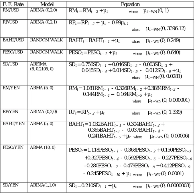
Table 1 presents the empirical results of the best fitting model for each of the transformed zero-mean stationary foreign exchange rate series.
Table 1: Best fitting model for each foreign exchange rate (1971: Q1 – 1997: Q2).
F. E. Rate Model Equation
RM/USD ARIMA (0,2,0) RMt = RMt –2 + µt where µt ~ WN (0, 1)
RP/USD ARIMA (0,2,1) RPt = RPt –2 + µt - 0.99µt-1
where µt ~ WN (0, 3396.12)
BAHT/USD RANDOM WALK BAHTt = BAHTt –1 + µt where µt ~ WN (0, 0.249) PESO/USD RANDOM WALK PESOt = PESOt –1 + µt where µt ~ WN (0, 0.640) SD/USD ARFIMA (6, 0.2105, 0) SD 0.045SDt = 0.756SDt –1 + 0.046SDt –2 - 0.003SDt –3 + t –4 + 0.014SDt –5 - 0.012SDt –6 + µt where µt ~ WN (0, 0.0281) RM/YEN ARMA (5, 0) RMt = 1.081RMt –1 - 0.326RMt –2 + 0.3884RMt –3 - 0.144RMt –4 – 0.164RMt –5 + µt where µt ~ WN (0, 0.000001)
RP/YEN ARIMA (0,2,0) RPt = RPt –2 + µt where µt ~ WN (0, 1.339) BAHT/YEN ARMA (5, 0) BAHTt = 1.032BAHTt –1 - 0.304BAHTt –2 +
0.365BAHTt –3 - 0.037BAHTt –4 -
0.241BAHTt –5 + µt where µt ~ WN (0, 0.00006)
PESO/YEN ARMA (10, 0)
PESOt = 1.118PESOt –1 - 0.368PESOt –2 + 0.150PESOt –3
+0.327PESOt –4 - 0.592PESOt –5 - 0.227PESOt –6
-0.280PESOt –7 - 0.479PESOt –8 + 0.412PESOt –9
-0.245PESOt –10 + µt where µt ~ WN (0, 0.0001) SD/YEN ARIMA(1,1,0) SDt = 0.210SDt –1 + µt where µt ~ WN (0, 0.0000003)
The Ljung-Box Q-statistic for 20 lags shows that there is no evidence of serial correlation for the residuals of the 5% level or better in each of these models, except for the RM/USD and RP/YEN series. However, the modified version of the Q-statistic, as formulated by McLeod and Li (1983) suggests that the residuals for these two series are from iid sequences and hence they are not serial correlated. The McLeod-Li Q-statistic uses squared-residual autocorrelations for testing whether the data are observations from
an iid sequence of normally distributed random variables. The results of diagnostic tests are summarized in the Appendix.
Eight actual and forecasted values for exchange rates denominated in US dollar from 1997: Q3 to 1999: Q2 for each model were plotted in Figure 1. Bearing in mind that in using any fitted model for forecasting, we assumed the economic fundamentals during the forecasting period remain the same as before. If this assumption holds, 95% of the actual exchange rate during this forecasting period lies inside our forecast interval. In other words, the actual observations would be what we have expected. However, as revealed by Figure 1, this was only true for Singapore dollar (Figure 1a). Perhaps it suggests that Singapore’s economic fundamentals remained unaltered following the recent financial crisis.
The best fitting model for SD/USD rate, ARFIMA (6, 0.2105,0) model, had MAPE, MAE and RMSE values of 26.469%, 1.006 and 0.00269% respectively. Furthermore, the actual observations had the correct trend of depreciation over the first 2 years following the crisis, as predicted. Nevertheless, the ARFIMA (6, 0.2105,0) model tends to overestimate the strength of Singapore dollar (Figure 1a).
Judging from the plots of Indonesia rupiah (Figure 1b), Thailand baht (Figure 1c) and the Philippines peso (Figure 1d) apparently had a different economic structure after the crisis, as their actual exchange rates during the forecasting period (after crisis) are totally beyond our expectation. Moreover, all these 3 currencies experienced an unexpectedly sharp depreciation, suggesting that most probably these countries were badly affected by the crisis.
For the case of Malaysia, ringgit denominated in US dollar (Figure 1e) had also experienced a worse-than-expected depreciation within the first year after the crisis. However, from 2 September 1998 onwards, exchange rate was fixed at RM3.80 per US dollar, a value lying within our model’s 95% forecast interval. We noted that under the
free floating system, the predicted values for ringgit in term of US dollar would be RM2.94 in 1999: Q2 and RM3.27 in 2000: Q4.
Figure 1: Actual and forecasted values of foreign exchange rates denominated in US dollar (1997: Q3 to 1999: Q2).
This result of this study is consistent with the real situation. Since the declaration of insolvency of various financial institutions in Thailand followed by the failure of a large Korean conglomerate in the year 1997, South Korea together with 4 Asean countries, namely Malaysia, Indonesia, Thailand and the Philippines were in trouble (Dunn and Mutti, 2000). Currencies of these countries plunged to its record low. For instance, Indonesian rupiah was more than 80 percent down against the U. S. Dollar, and the currencies of Thailand, South Korea, Malaysia and the Philippines all dived by 35 to 50 percent (Carbaugh, 2000). However, the Singapore appears largely unaffected by the crisis.
Next, we modeled the Asean currencies against the Japanese yen. The actual and forecasted values of foreign exchange rates denominated in Japanese yen were shown in Figure 2. By comparing Figures 1 and 2, we found that in general, the forecasts using models based on yen outperformed the models based on US dollar. Figure 2a showed that the forecasted values of Singapore dollar denominated in yen fall in the 95% confident interval. Singapore dollar is the only Asean currencies that remain predictable in both US dollar and Japanese yen bases models. It appears that exchange rate had little success in predicting the currencies crisis.
Figures 2b, 2c and 2d revealed that the first two quarters after the crisis for the predicted peso, bath and the ringgit failed to be in the 95% confident interval. Specifically, the models mis-predict by more than 25% in the short term. Particularly the models consistently over-predicts in the short term. We noted that the out-sample forecasts are within 95% confident level after the third quarter, suggesting that our model based on Japanese yen is more appropriate in the medium to long term. As for rupiah, although model based on yen (Figure 2e) performed better than that of US dollar, only the forecast after 7-quarter horizon fall in the 95% confident interval.
Figure 2: Actual and forecasted values of foreign exchange rates denominated in Japanese yen (1997: Q3 to 1999: Q2).
The performance of models based on US dollar and Japanese yen is summarized in Table 2. As we have noted earlier, the pre-crisis period (1971: Q1 to 1997: Q2) is used to fit the model, while the post-crisis period (1977: Q3 to 1999: Q2) is kept for post sample forecasting. Two important conclusions may be drawn from this table. Firstly, a
quick flash at the overall results showed that, the performance of the best fitting models had deteriorated in the post-crisis period. Upon comparing the performance term by term, it is clear that in fact all the models did not turn out to be as predictive as they were. As we have noted earlier, this phenomenon might be attributed to the set in of the Asian Financial crisis.
Table 2: Performance of best-fitting models for various exchange rates (Sample period: 1971: Q1 to 1999: Q2)
PERIOD PRE-CRISIS (1971: Q1 to 1997: Q2) POST-CRISIS (1997: Q3 to 1999: Q2)
F. E. RATE MAPE (%) MAE* RMSE (%) MAPE (%) MAE* RMSE (%)
RM/USD 2.794 0.069 0.00039 26.469 1.006 0.00269 RM/YEN 4.930 0.001 0.00061 8.260 0.002 0.00103 PESO/USD 0.624 0.164 0.00007 45.939 33.716 0.00503 PESO/YEN 4.200 0.012 0.00061 7.567 0.023 0.00086 RP/USD 0.520 12.213 0.00008 61.531 5550.088 0.00640 RP/YEN 4.668 1.009 0.00070 46.040 33.162 0.00621 SD/USD 0.910 0.013 0.00014 3.711 0.062 0.00047 SD/YEN 4.926 0.001 0.00064 5.439 0.001 0.00064 BAHT/USD 0.601 0.150 0.00008 33.574 13.423 0.00340 BAHT/YEN 5.138 0.012 0.00062 7.729 0.025 0.00102 OVERALL 2.931 1.364 .000039 24.626 563.15 0.00280
* MAE is not suitable for comparing intra-period models of different exchange series, as it is a measure of absolute (not relative) deviation from the actual observations. It is relevant for comparing inter-period models of the same exchange rate series, however.
The second obvious feature in Table 2 is that models (except for Singapore dollar) denominated in Japanese yen outperformed their counterparts in the post-crisis period. Putting aside the MAE criterion, which is not relevant for comparing intra-period models, all the other accuracy criteria showed that models (except for Singapore dollar) based on yen are more accurate in forecasting, than models based on US dollar. For instance, quoted per US dollar, the RMSE percentages for ringgit, peso, rupiah, and bath were 0.00269, 0.00503, 0.00640, and 0.00109 respectively. These values were much higher
than their corresponding values based on yen, i.e. 0.00103, 0.00503, 0.00640 and 0.00102 respectively. The RMSE percentages for SD/USD and SD/YEN were 0.00047 and 0.00069 respectively. However, for the pre-crisis period, obvious that the US dollar denominator is better than the Japanese yen, is better. This is because we have MAPE and RMSE (%) criteria showing that for all the exchange rates under this study, the models based on US dollar denominator had performed better prediction.
The correlation between the actual observations of each exchange rate series and their corresponding best fitting model’s predicted values is depicted in Table 3. All the correlations for pre-crisis period are significant at 1% level, with values ranging from 0.887 for the case of RM/USD rate, to 0.997 for the case of RP/USD rate. However, for the post-crisis period, only 40% of the computed correlations are significantly at 5% level. These include RM/YEN (0.739), PESO/YEN (0.714), SD/YEN (0.734) and SD/USD (0.748) rates. This decrease in the degree of correlation for the post-crisis period is synonym to the deterioration of the performance of the model in term of tracking the movement of the exchange rates in the post-crisis period.
Table 3: Correlation between actual values and predicted values. PERIOD PRE-CRISIS POST-CRISIS
F. E. RATE CORRELATION p - VALUE CORRELATION p - VALUE
RM/USD 0.887** 0.000 0.406 0.318 RM/YEN 0.991** 0.000 0.739* 0.036 PESO/USD 0.995** 0.000 0.433 0.283 PESO/YEN 0.994** 0.000 0.714* 0.047 RP/USD 0.997** 0.000 0.357 0.385 RP/YEN 0.989** 0.000 0.435 0.281 SD/USD 0.989** 0.000 0.748* 0.033 SD/YEN 0.976** 0.000 0.734* 0.038 BAHT/USD 0.989** 0.000 -0.428 0.291 BAHT/YEN 0.993** 0.000 -0.224 0.594 * *Correlation is significant at 1% level (2-tailed).
Consistent also, with the second feature that we observed earlier on, Table 3 showed that the yen could be a better denominator for the ringgit, peso, rupiah and bath but not for Singapore dollar, for the post-crisis period. The correlations for the RM/YEN, PESO/YEN, RP/YEN and BAHT/YEN rates are respectively 0.739, 0.714, 0.435 and – 0.224 and are higher than their correspondences, i.e. 0.406, 0.439, 0.357 and –0.428. The correlation for the SD/USD rate (0.748) is higher than SD/YEN rate (0.734), however.
It was obvious, that except for Singapore dollar, the forecasting performance of all other models for Asean currencies denominated in yen had outperformed those denominated in US dollar. Yen is therefore a better measurement unit of Asean exchange rates, as compare to US dollar, at least for the post-crisis period, a more recent time horizon. One of the plausible explanations for this would be Japan and the other Asean countries in this study (except Singapore), had undergone various degree of economical recession after the crisis. Similarly, US dollar could serve to measure Singapore dollar better mostly because both countries were large unaffected by the crisis. Yen, however was still a poor measurement unit for rupiah perhaps due to the fact that after the currency crisis, Japan although was caught in a serious recession in 1998 (Dunn and Mutti, 2000) it did not experienced similar political instability as experienced by Indonesia. This is supportive to the statement made by McKibbin (1998): The impact of politics on Indonesia’s economics is so striking that without the reference to the political situation, it was not possible to understand Indonesia’s economics.
6. Conclusion
Five Asean currencies including Malaysian ringgit, Thailand bath, Singapore dollar, Indonesian rupiah and the Philippines peso, denominated in US dollar as well as Japanese yen, were modeled in this study using advanced time series analysis. Results suggested that Singapore dollar is better predicted when denominated in US dollar. This
Similarly, other Asean exchange rates were better predicted when denominated in Japanese yen, as they had closer economic ties with Japan. However, while Japan had undergone serious recession after the crisis, it did not experience dramatic political instability as experienced by Indonesia. Hence, the Indonesian rupiah remained unpredictable by yen. In all the financial crisis countries (Indonesia, Malaysia, the Philippines and Thailand), the period of sharp declined ended by February 1998. The period of free fall was largest and deepest in Indonesia, which was the only country to experience political uncertainties as well. This makes financial stability hard to ascertain (see Mei, 1999). This free fall is reflected in Figures 1 and 2 in that the divergence between the predicted and the actual rates appears to be largest in Indonesia. These results show that although advanced time series analysis dealt with economic fundamentals implicitly, it could be a powerful tool for exchange rates modeling and forecasting, especially in the medium to long term.
References
1. Berkowitz, J. and Giogianni, L. (1997), ‘Long –horizon exchange rate predictability?’, Working Paper of the Internatinonal Monetary Fund, International Monetary Fund, WP/97/6.
2. Brockwell, P. J. and Davis, R. A. (1996), Introduction To Time Series and
Forecasting, Springer, U. S.
3. Brooks, C. (1997), ‘Linear and Non-linear (Non-) Forcastability of high-frequency
exchange rates’, Journal of Forecasting, Vol. 16, 125 – 145.
4. Carbaugh, R. J. (2000), International Economics, 7th edition, International Thomson
5. Cheung, Y. W. (1993), ‘Long memory in foreign-exchange rates’, Journal of Bussiness and Economics studies, 11, 93 – 101.
6. Dunn, R. M. and Mutti, J. H. (2000), International Economics, 5th edition, Routledge,
London.
7. Fatimah Mhd. Arshad and Gaffar, R. A. (1986), ‘Univariate approach towards cocoa
price forecasting’, The Malaysian Journal of Agricultural Economics, 3, 1 – 11.
8. Berkowitz, J. and Giorgianni, J. (1997), ‘Long-horizon exchange rate predictability?’, Working Paper of the International Monetary Fund.
9. García-Ferrer, A., Del Hoyo, J. and Martín-Arroyo, A. S. (1997), ‘Univariate
forecasting comparisons: The case of the Spanish automobile industry’, Journal of
Forecasting, Vol. 16, 1 – 17.
10. Keller, A. (1989), ‘Advanced time-series analysis’, in Dunis, C. and Feeny, M.
(1989), eds., Exchange Rate Forecasting, Woodhead-Faulkner, England, 206 – 99.
11. Lalang B~A. M. Razali and I-L J. Zoinodin (1997), Performance of Some
Forecasting Techniques Applied on Palm Oil Price Data, Prosiding Institut Stasistik
Malaysia (20-9-1997), 82 –92.
12. Liew, K. S. (2000), ‘The performance of minimum AICC as order selection
criterion for time series modelling’, project paper, Mathematics Department,
Universiti Putra Malaysia, Kuala Lumpur.
14. Lupoletti, W. M. and Webb, R. H. (1986), ‘Defining and improving the accuracy of
macroeconomics forecasts: contribution of a VAR model’, Journal of Business,
vol. 59, 263-84.
15. Makridakis, S. and Hobon, M. (1997), ‘ARMA models and the Box-Jenkins
methodology’, Journal of Forecasting, Vol. 16, 147 – 163.
16. McLeod, A. I. And Li, W. K. (1983), ‘Diagnostic checking ARMA time series
models using squared-residual autotegressions’, Journal of Time Series Annals, 4,
269 – 273.
17. McKibbin, W. (1998), ‘Modelling the Crisis in Asia’, ASEAN Economic Bulletin, vol.
15, 3, 347 – 52.
18. Meese, R and Rogoff, K (1983), ‘Empirical exchange rate models of the seventies: do
they fit out of sample?’, Journal of International Economics, vol. 14, 3 – 24.
19. Mei, J. (1998), ‘Political risk, financial crisis and market volatility’, unpublished
paper, New York University Department of Finance, New York.
20. Montogomery, D. C., Johnson, L. A. and Gardiner, J. S. (1990), ‘Autoregressive
Intergrated Moving Average models, Forecasting and Time Series Analysis, 2nd
edition, McGraw-Hill Inc., U. S.
21. Palma, W. and Chan, N. H. (1997), ‘Estimation and forecasting of long-memory
processes with missing values’, Journal of Forecasting, Vol. 16, 395-410.
22. Shitan, M. and Liew, K. S. (2000), ‘Time series modelling of Sarawak black
pepper price’, unpublished paper, Mathematics Department, Universiti Putra
23. Six, J. M. (1989), ‘Economics and exchange rate forecasts’, in Dunis, C. and
Feeny, M. (1989), eds., Exchange Rate Forecasting, Woodhead-Faulkner, England,
21 – 44.
24. Wolf, C. P. P. (1978), ‘Time-varying parameters and the out-sample forecasting
performance of structural exchange models’, Journal of Business and Economics
Statistics, 5, 87 – 97.
25. Zhou, S. H. (1998), ‘Exchange rate systems and linkages in the Pacific Basin’, Asian
Appendix
Diagnostic Test Results for Various Exchange Rates
Exchange rate: RM / USD Model: ARIMA ( 0, 2, 0 ) Ljung-Box Q-statistic = 43.62 X2.05, 20= 31.41
McLeod-Li Q-statistic = 31.39 X2.05, 20= 31.41 Turning Points = 70 iid ( 68.0, 4.262 ) Difference-sign = 53 iid ( 57.5, 2.962 ) Rank Test = 2561 iid (2678.0, 534.52 ) Order of minimum AICC model for residuals = 6
Exchange rate: RP / USD Model: ARIMA (0 , 2, 1 ) Ljung-Box Q-statistic = 17.99 X2.05, 20= 31.41
McLeod-Li Q-statistic = 8.04 X2.05, 21= 32.67 Turning Points = 50 iid ( 68.0, 4.26 2 ) Difference-sign = 50 iid ( 51.5, 2.962 ) Rank Test = 2207 iid ( 2678.0, 534.12 ) Order of minimum AICC model for residuals = 0
Exchange rate: BAHT / USD Model: Random Walk Ljung-Box Q-statistic = 26.74 X2.05, 20= 31.41 McLeod-Li Q-statistic = 5.74 X2.05, 20= 31.41 Turning Points = 41 iid ( 68.7, 4.282 ) Difference-sign = 37 iid ( 52.0, 2.972 ) Rank Test = 2307 iid ( 2730.0, 541.82 ) Order of minimum AICC model for residuals = 0
Exchange rate: PESO / USD Model: Random Walk Ljung-Box Q-statistic = 30.43 X2.05, 20= 31.41 McLeod-Li Q-statistic = 24.78 X2.05, 21= 32.67 Turning Points = 66 iid ( 68.7, 4.282 ) Difference-sign = 55 iid ( 52.0, 2.972 ) Rank Test = 3012 iid ( 2730, 541.82 ) Order of minimum AICC model for residuals = 3
Exchange rate: RM / YEN Model: ARMA ( 5, 0 ) Ljung-Box Q-statistic = 20.38 X2.05, 20= 31.41 McLeod-Li Q-statistic = 35.92 X2.05, 25= 37.65 Turning Points = 73 iid ( 69.3, 4.302 ) Difference-sign = 53 iid ( 52.5, 2.952 ) Rank Test = 2681 iid (2782.5, 549.52 ) Order of minimum AICC model for residuals = 0
Exchange rate: RP / YEN Model: ARIMA ( 0, 2, 0 ) Ljung-Box Q-statistic = 48.71 X2.05, 20= 31.41 McLeod-Li Q-statistic = 23.18 X2.05, 20= 31.41 Turning Points = 73 iid ( 68.0, 4.262 ) Difference-sign = 54 iid ( 51.5, 2.962 ) Rank Test = 2688 iid ( 2678.0, 534.12 ) Order of minimum AICC model for residuals = 3
Exchange rate: BAHT / YEN Model: ARMA (5, 0 ) Ljung-Box Q-statistic = 11.67 X2.05, 20= 31.41 McLeod-Li Q-statistic = 26.27 X2.05, 25= 37.65 Turning Points = 73 iid ( 69.3, 4.302 ) Difference-sign = 50 iid ( 52.5, 2.992 ) Rank Test = 2728 iid ( 2782.0, 549.52 ) Order of minimum AICC model for residuals = 0
Exchange rate: PESO / YEN Model: ARMA (10, 0 ) Ljung-Box Q-statistic = 23.34 X2.05, 20= 31.41 McLeod-Li Q-statistic = 98.67 X2.05, 30= 43.77 Turning Points = 77 iid ( 69.3, 4.302 ) Difference-sign = 53 iid ( 52.5, 2.992 ) Rank Test = 2386 iid (2782.0, 549.52 ) Order of minimum AICC model for residuals = 0
Exchange rate: SD / YEN Model: ARIMA ( 1, 1, 0 ) Ljung-Box Q-statistic = 31.78 X2.05, 20= 31.41
McLeod-Li Q-statistic = 15.77 X2.05, 21= 32.67 Turning Points = 64 iid ( 68.7, 4.282 ) Difference-sign = 53 iid ( 52.5, 2.972 ) Rank Test = 2656 iid ( 2730.0, 541.82 ) Order of minimum AICC model for residuals = 0