Predicting Bankruptcy with Support Vector Machines

(1)

SFB 649 Discussion Paper 2005-009

Predicting Bankruptcy

with Support Vector

Machines

Wolfgang Härdle*

Rouslan A. Moro* **

Dorothea Schäfer**

* CASE - Center for Applied Statistics and Economics, Humboldt-Universität zu Berlin, Germany ** German Institute for Economic Research (DIW),

Berlin, Germany

This research was supported by the Deutsche

Forschungsgemeinschaft through the SFB 649 "Economic Risk". http://sfb649.wiwi.hu-berlin.de ISSN 1860-5664

S

FB

6

4

9 E

C

O

N

O

M

I

C

R

I

S

K

B

E

R

L

I

N

(2)

1 Predicting bankruptcy with

Support Vector Machines

Wolfgang H¨ardle,Rouslan Moro,Dorothea Sch¨afer

The purpose of this work is to introduce one of the most promising among re-cently developed statistical techniques – the support vector machine (SVM) – to corporate bankruptcy analysis. An SVM is implemented for analysing such predictors as financial ratios. A method of adapting it to default probability estimation is proposed. A survey of practically applied methods is given. This work shows that support vector machines are capable of extracting useful infor-mation from financial data, although extensive data sets are required in order to fully utilize their classification power.

The support vector machine is a classification method that is based on sta-tistical learning theory. It has already been successfully applied to optical character recognition, early medical diagnostics, and text classification. One application where SVMs outperformed other methods is electric load prediction (EUNITE, 2001), another one is optical character recognition (Vapnik, 1995). SVMs produce better classification results than parametric methods and such a popular and widely used nonparametric technique as neural networks, which is deemed to be one of the most accurate. In contrast to the latter they have very attractive properties. They give a single solution characterized by the global minimum of the optimized functional and not multiple solutions associ-ated with the local minima as in the case of neural networks. Moreover, SVMs do not rely so heavily on heuristics, i.e. an arbitrary choice of the model and have a more flexible structure.

1.1 Bankruptcy analysis methodology

Although the early works in bankruptcy analysis were published already in the 19th century (Dev, 1974), statistical techniques were not introduced to it until the publications of Beaver (1966) and Altman (1968). Demand from

(3)

finan-cial institutions for investment risk estimation stimulated subsequent research. However, despite substantial interest, the accuracy of corporate default predic-tions was much lower than in the private loan sector, largely due to a small number of corporate bankruptcies.

Meanwhile, the situation in bankruptcy analysis has changed dramatically. Larger data sets with the median number of failing companies exceeding 1000 have become available. 20 years ago the median was around 40 companies and statistically significant inferences could not often be reached. The spread of computer technologies and advances in statistical learning techniques have allowed the identification of more complex data structures. Basic methods are no longer adequate for analysing expanded data sets. A demand for advanced methods of controlling and measuring default risks has rapidly increased in anticipation of the New Basel Capital Accord adoption (BCBS, 2003). The Accord emphasises the importance of risk management and encourages im-provements in financial institutions’ risk assessment capabilities.

In order to estimate investment risks one needs to evaluate the default prob-ability (PD) for a company. Each company is described by a set of variables (predictors)x, such as financial ratios, and its classythat can be eithery=−1 (‘successful’) or y = 1 (‘bankrupt’). Initially, an unknown classifier function

f :x→y is estimated on a training set of companies (xi, yi),i= 1, ..., n. The training set represents the data for companies which are known to have sur-vived or gone bankrupt. Finally,f is applied to computing default probabilities (PD) that can be uniquely translated into a company rating.

The importance of financial ratios for company analysis has been known for more than a century. Among the first researchers applying financial ratios for bankruptcy prediction were Ramser (1931), Fitzpatrick (1932) and Winakor and Smith (1935). However, it was not until the publications of Beaver (1966) and Altman (1968) and the introduction of univariate and multivariate discrim-inant analysis that the systematic application of statistics to bankruptcy analy-sis began. Altman’s linear Z-score model became the standard for a decade to come and is still widely used today due to its simplicity. However, its assump-tion of equal normal distribuassump-tions for both failing and successful companies with the same covariance matrix has been justly criticized. This approach was further developed by Deakin (1972) and Altman et al. (1977).

Later on, the center of research shifted towards the logit and probit models. The original works of Martin (1977) and Ohlson (1980) were followed by (Wiginton, 1980), (Zavgren, 1983) and (Zmijewski, 1984). Among other statistical methods applied to bankruptcy analysis there are the gambler’s ruin model (Wilcox,

(4)

1.1 Bankruptcy analysis methodology

1971), option pricing theory (Merton, 1974), recursive partitioning (Frydman et al., 1985), neural networks (Tam and Kiang, 1992) and rough sets (Dimitras et al., 1999) to name a few.

There are three main types of models used in bankruptcy analysis. The first one is structural or parametric models, e.g. the option pricing model, logit and probit regressions, discriminant analysis. They assume that the relationship between the input and output parameters can be describeda priori. Besides their fixed structure these models are fully determined by a set of parameters. The solution requires the estimation of these parameters on a training set. Although structural models provide a very clear interpretation of modelled processes, they have a rigid structure and are not flexible enough to capture information from the data. The non-structural or nonparametric models (e.g. neural networks or genetic algorithms) are more flexible in describing data. They do not impose very strict limitations on the classifier function but usually do not provide a clear interpretation either.

Between the structural and non-structural models lies the class of semipara-metric models. These models, like the RiskCalc private company rating model developed by Moody’s, are based on an underlying structural model but all or some predictors enter this structural model after a nonparametric transforma-tion. In recent years the area of research has shifted towards non-structural and semi-parametric models since they are more flexible and better suited for practical purposes than purely structural ones.

Statistical models for corporate default prediction are of practical importance. For example, corporate bond ratings published regularly by rating agencies such as Moody’s or S&P strictly correspond to company default probabilities estimated to a great extent statistically. Moody’s RiskCalc model is basically a probit regression estimation of the cumulative default probability over a number of years using a linear combination of non-parametrically transformed predic-tors (Falkenstein, 2000). These non-linear transformations f1, f2, ..., fd are estimated on univariate models. As a result, the original probit model:

E[yi,t|xi,t] = Φ (β1xi1,t+β2xi2,t+...+βdxid,t), (1.1) is converted into:

E[yi,t|xi,t] = Φ{β1f1(xi1,t) +β2f2(xi2,t) +...+βdfd(xid,t)}, (1.2) whereyi,tis the cumulative default probability within the prediction horizon for companyiat timet. Although modifications of traditional methods like probit

(5)

analysis extend their applicability, it is more desirable to base our methodology on general ideas of statistical learning theory without making many restrictive assumptions.

The ideal classification machine applying a classifying function f from the available set of functionsFis based on the so called expected risk minimization principle. The expected risk

R(f) = Z ₁

2|f(x)−y|dP(x, y), (1.3) is estimated under the distributionP(x, y), which is assumed to be known. This is, however, never true in practical applications and the distribution should also be estimated from the training set (xi, yi),i= 1,2, ..., n, leading to an ill-posed problem (Tikhonov and Arsenin, 1977).

In most methods applied today in statistical packages this problem is solved by implementing another principle, namely the principle of the empirical risk minimization, i.e. risk minimization over the training set of companies, even when the training set is not representative. The empirical risk defined as:

ˆ R(f) = 1 n n X i=1 1 2|f(xi)−yi|, (1.4) is nothing else but an average value of loss over the training set, while the expected risk is the expected value of loss under the true probability measure. The loss for i.i.d. observations is given by:

1

2|f(x)−y|= (

0, if classification is correct, 1, if classification is wrong.

The solutions to the problems of expected and empirical risk minimization:

fopt = arg min

f∈FR(f), (1.5) ˆ fn = arg min f∈F ˆ R(f), (1.6)

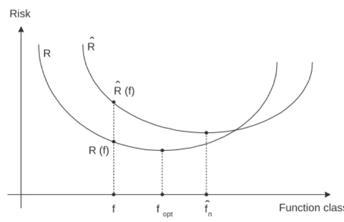
generally do not coincide (Figure 1.1), although converge asn→ ∞ifF is not too large.

We can not minimize expected risk directly since the distribution P(x, y) is unknown. However, according to statistical learning theory (Vapnik, 1995), it

(6)

1.1 Bankruptcy analysis methodology Function class Risk f f_opt R R(f) f_n ˆ Rˆ(f) Rˆ

Figure 1.1: The minima fopt and ˆfn of the expected (R) and empirical ( ˆR) risk functions generally do not coincide.

is possible to estimate the Vapnik-Chervonenkis (VC) bound that holds with a certain probability 1−η: R(f)≤Rˆ(f) +φ h n, ln(η) n . (1.7)

For a linear indicator functiong(x) = sign(x⊤_w₊_b_):

φ _h n, ln(η) n = s h ln2n h −lnη₄ n , (1.8)

wherehis the VC dimension.

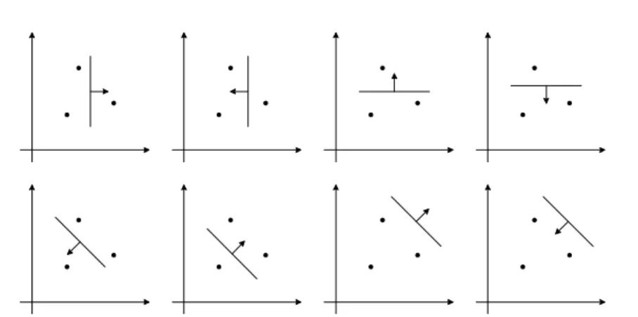
The VC dimension of the function setF in ad-dimensional space is hif some function f ∈ F can shatter h objects

xi∈Rd, i= 1, ..., h , in all 2h possi-ble configurations and no set

xj ∈Rd, j= 1, ..., q , exists whereq > h that satisfies this property. For example, three points on a plane (d = 2) can be shattered by linear indicator functions in 2h _{= 2}3_{= 8 ways, whereas 4 points} can not be shattered in 2q = 24= 16 ways. Thus, the VC dimension of the set of linear indicator functions in a two-dimensional space is three, see Figure 1.2. The expression for the VC bound (1.7) is a regularized functional where the VC dimensionhis a parameter controlling complexity of the classifier function. The

(7)

Figure 1.2: Eight possible ways of shattering 3 points on the plane with a linear indicator function.

termφh n,

ln(η)

n

introduces a penalty for the excessive complexity of a classifier function. There is a trade-off between the number of classification errors on the training set and the complexity of the classifier function. If the complexity were not controlled, it would be possible to find such a classifier function that would make no classification errors on the training set notwithstanding how low its generalization ability would be.

1.2 Importance of risk classification in practice

In most countries only a small percentage of firms has been rated to date. The lack of rated firms is mainly due to two factors. Firstly, an external rating is an extremely costly procedure. Secondly, until the recent past most banks decided on their loans to small and medium sized firms (SME) without asking for the client’s rating figure or applying an own rating procedure to estimate the client’s default risk. At best, banks based their decision on rough scoring models. At worst, the credit decision was completely left to the loan officer. Since learning to know its own risk is costly and, until recently, the lending procedure of banks failed to set the right incentives, small and medium sized firms shied away from rating. However, the regulations are about to change the environment for borrowing and lending decisions. With the implementation of

(8)

1.2 Importance of risk classification in practice

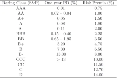
Rating Class (S&P) One year PD (%) Risk Premia (%)

AAA 0.01 0.75 AA 0.02 – 0.04 1.00 A+ 0.05 1.50 A 0.08 1.80 A- 0.11 2.00 BBB 0.15 – 0.40 2.25 BB 0.65 – 1.95 3.50 B+ 3.20 4.75 B 7.00 6.50 B- 13.00 8.00 CCC >13 10.00 CC 11.50 C 12.70 D 14.00

Table 1.1: Rating grades and risk premia. Source: (Damodaran, 2002) and (F¨user, 2002)

the New Basel Capital Accord (Basel II) scheduled for the end of 2006 not only firms that issue debt securities on the market are in need of rating but also any ordinary firm that applies for a bank loan. If no external rating is available, banks have to employ an internal rating system and deduce each client’s specific risk class. Moreover, Basel II puts pressure on firms and banks from two sides.

First, banks have to demand risk premia in accordance to the specific borrower’s default probability. Table 1.1 presents an example of how individual risk classes map into risk premiums (Damodaran, 2002) and (F¨user, 2002). For small US-firms a one-year default probability of 0.11% results in a spread of 2%. Of course, the mapping used by lenders will be different if the firm type or the country in which the bank is located changes. However, in any case future loan pricing has to follow the basic rule. The higher the firm’s default risk is the more risk premium the bank has to charge.

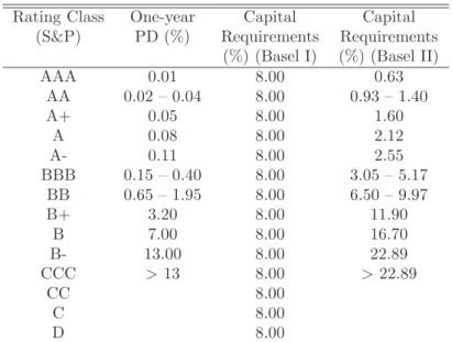
Second, Basel II requires banks to hold client-specific equity buffers. The mag-nitudes of these buffers are determined by a risk weight function defined by the Basel Committee and a solvability coefficient (8%). The function maps default probabilities into risk weights. Table 1.2 illustrates the change in the

(9)

Rating Class One-year Capital Capital (S&P) PD (%) Requirements Requirements

(%) (Basel I) (%) (Basel II)

AAA 0.01 8.00 0.63 AA 0.02 – 0.04 8.00 0.93 – 1.40 A+ 0.05 8.00 1.60 A 0.08 8.00 2.12 A- 0.11 8.00 2.55 BBB 0.15 – 0.40 8.00 3.05 – 5.17 BB 0.65 – 1.95 8.00 6.50 – 9.97 B+ 3.20 8.00 11.90 B 7.00 8.00 16.70 B- 13.00 8.00 22.89 CCC >13 8.00 >22.89 CC 8.00 C 8.00 D 8.00

Table 1.2: Rating grades and capital requirements. Source: (Damodaran, 2002) and (F¨user, 2002). The figures in the last column were es-timated by the authors for a loan to an SME with a turnover of 5 million euros with a maturity of 2.5 years using the data from col-umn 2 and the recommendations of the Basel Committee on Banking Supervision (BCBS, 2003).

capital requirements per unit of a loan induced by switching from Basel I to Basel II. Apart from basic risk determinants such as default probability (PD), maturity and loss given default (LGD) the risk weights depend also on the type of the loan (retail loan, loan to an SME, mortgages, etc.) and the annual turnover. Table 1.2 refers to an SME loan and assumes that the borrower’s annual turnover is 5 million EUR (BCBS, 2003). Since the lock-in of the bank’s equity affects the provision costs of the loan, it is likely that these costs will be handed over directly to an individual borrower.

Basel II will affect any firm that is in need for external finance. As both the risk premium and the credit costs are determined by the default risk, the firms’ rating will have a deeper economic impact on banks as well as on firms themselves than ever before. Thus in the wake of Basel II the choice of the right

(10)

1.3 Lagrangian formulation of the SVM

rating method is of crucial importance. To avoid friction of a large magnitude the employed method must meet certain conditions. On the one hand, the rating procedure must keep the amount of misclassifications as low as possible. On the other, it must be as simple as possible and, if employed by the borrower, also provide some guidance to him on how to improve his own rating.

SVMs have the potential to satisfy both demands. First, the procedure is easy to implement so that any firm could generate its own rating information. Second, the method is suitable for estimating a unique default probability for each firm. Third, the rating estimation done by an SVM is transparent and does not depend on heuristics or expert judgements. This property implies objectivity and a high degree of robustness against user changes. Moreover, an appropriately trained SVM enables the firm to detect the specific impact of all rating determinants on the overall classification. This property would enable the firm to find out prior to negotiations what drawbacks it has and how to overcome its problems. Overall, SVMs employed in the internal rating systems of banks will improve the transparency and accuracy of the system. Both improvements may help firms and banks to adapt to the Basel II framework more easily.

1.3 Lagrangian formulation of the SVM

Having introduced some elements of statistical learning and demonstrated the potential of SVMs for company rating we can now give a Lagrangian formula-tion of an SVM for the linear classificaformula-tion problem and generalize this approach to a nonlinear case.

In the linear case the following inequalities hold for allnpoints of the training set:

x⊤i w+b≥1−ξi for yi= 1,

x⊤

i w+b≤ −1 +ξi for yi=−1,

ξi≥0, which can be combined into two constraints:

yi(x⊤i w+b)≥1−ξi (1.9)

ξi≥0. (1.10)

(11)

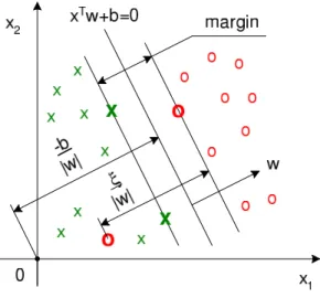
Figure 1.3: The separating hyperplanex⊤_w₊_b_{= 0 and the margin in a}

non-separable case.

that corresponds to the largest possible margin between the points of different classes, see Figure 1.3. Some penalty for misclassification must also be intro-duced. The classification errorξiis related to the distance from a misclassified point xi to the canonical hyperplane bounding its class. If ξi > 0, an error in separating the two sets occurs. The objective function corresponding to penalized margin maximization is formulated as:

1 2kwk 2 +C n X i=1 ξi !υ , (1.11)

where the parameterCcharacterizes the generalization ability of the machine andυ≥1 is a positive integer controlling the sensitivity of the machine to out-liers. The conditional minimization of the objective function with constraint (1.9) and (1.10) provides the highest possible margin in the case when classi-fication errors are inevitable due to the linearity of the separating hyperplane. Under such a formulation the problem is convex. One can show that margin maximization reduces the VC dimension.

(12)

1.3 Lagrangian formulation of the SVM

The Lagrange functional for the primal problem forυ= 1 is:

LP = 1 2kwk 2 +C n X i=1 ξi− n X i=1 αi{yi x⊤i w+b −1 +ξi} − n X i=1 µiξi, (1.12) where αi ≥ 0 and µi ≥ 0 are Lagrange multipliers. The primal problem is formulated as: min wk,b,ξi max αi LP.

After substituting the Karush-Kuhn-Tucker conditions (Gale et al., 1951) into the primal Lagrangian, we derive the dual Lagrangian as:

LD= n X i=1 αi− 1 2 n X i=1 n X j=1 αiαjyiyjx⊤i xj, (1.13)

and the dual problem is posed as: max αi LD, subject to: 0≤αi ≤C, n X i=1 αiyi = 0.

Those pointsifor which the equationyi(x⊤i w+b)≤1 holds are called support vectors. After training the support vector machine and deriving Lagrange multipliers (they are equal to 0 for non-support vectors) one can classify a company described by the vector of parametersxusing the classification rule:

g(x) = sign x⊤w+b

, (1.14)

wherew=Pn_i₌₁αiyixiandb= ₂1(x+1+x−1)w. x+1andx−1are two support vectors belonging to different classes for whichy(x⊤_w₊_b_{) = 1. The value of}

the classification function (the score of a company) can be computed as

f(x) =x⊤w+b. (1.15)

(13)

The SVMs can also be easily generalized to the nonlinear case. It is worth noting that all the training vectors appear in the dual Lagrangian formulation only as scalar products. This means that we can apply kernels to transform all the data into a high dimensional Hilbert feature space and use linear algorithms there:

Ψ :Rd7→H. (1.16)

If a kernel functionK exists such that K(xi, xj) = Ψ(xi)⊤Ψ(xj), then it can be used without knowing the transformation Ψ explicitly. A necessary and sufficient condition for a symmetric function K(xi, xj) to be a kernel is given by Mercer’s (1909) theorem. It requires positive definiteness, i.e. for any data setx1, ..., xn and any real numbersλ1, ..., λn the functionK must satisfy

n X i=1 n X j=1 λiλjK(xi, xj)≥0. (1.17) Some examples of kernel functions are:

• K(xi, xj) =e−kxi−xjk/2σ

2

– the isotropic Gaussian kernel; • K(xi, xj) = e−(xi−xj)

⊤_r−2_Σ−1₍_x

i−xj)/2 – the stationary Gaussian kernel

with an anisotropic radial basis; we will apply this kernel in our study taking Σ equal to the variance matrix of the training set;ris a constant; • K(xi, xj) = (x⊤i xj+ 1)P – the polynomial kernel;

• K(xi, xj) = tanh(kx⊤i xj−δ) – the hyperbolic tangent kernel.

1.4 Description of data

For our study we selected the largest bankrupt companies with the capitaliza-tion of no less than $1 billion that filed for proteccapitaliza-tion against creditors under Chapter 11 of the US Bankruptcy Code in 2001–2002 after the stock marked crash of 2000. We excluded a few companies due to incomplete data, leaving us with 42 companies. They were matched with 42 surviving companies with the closest capitalizations and the same US industry classification codes avail-able through the Division of Corporate Finance of the Securities and Exchange Commission (SEC, 2004).

(14)

1.5 Computational results

From the selected 84 companies 28 belonged to various manufacturing tries, 20 to telecom and IT industries, 8 to energy industries, 4 to retail indus-tries, 6 to air transportation indusindus-tries, 6 to miscellaneous service indusindus-tries, 6 to food production and processing industries and 6 to construction and con-struction material industries. For each company the following information was collected from the annual reports for 1998–1999, i.e. 3 years prior to defaults of bankrupt companies (SEC, 2004): (i) S – sales; (ii) COGS – cost of goods sold; (iii) EBIT – earnings before interest and taxes, in most cases equal to the oper-ating income; (iv) Int – interest payments; (v) NI – net income (loss); (vi) Cash – cash and cash equivalents; (vii) Inv – inventories; (viii) CA – current assets; (ix) TA – total assets; (x) CL – current liabilities; (xi) STD – current maturities of the long-term debt; (xii) TD – total debt; (xiii) TL – total liabilities; (xiv) Bankr – bankruptcy (1 if a company went bankrupt,−1 otherwise).

The information about the industry was summarized in the following dummy variables: (i) Indprod – manufacturing industries; (ii) Indtelc – telecom and IT industries; (iii) Indenerg – energy industries; (iv) Indret – retail industries; (v) Indair – air transportation industries; (vi) Indserv – miscellaneous service industries; (vii) Indfood – food production and processing industries; (viii) Indconst – construction and construction material industries.

Based on these financial indicators the following four groups of financial ratios were constructed and used in our study: (i) profit measures: EBIT/TA, NI/TA, EBIT/S; (ii) leverage ratios: EBIT/Int, TD/TA, TL/TA; (iii) liquidity ratios: QA/CL, Cash/TA, WC/TA, CA/CL and STD/TD, where QA is quick assets and WC is working capital; (iv) activity or turnover ratios: S/TA, Inv/COGS.

1.5 Computational results

The most significant predictors suggested by the discriminant analysis belong to profit and leverage ratios. To demonstrate the ability of an SVM to extract information from the data, we will chose two ratios from these groups: NI/TA from the profitability ratios and TL/TA from the leverage ratios. The SVMs, besides their Lagrangian formulation, can differ in two aspects: (i) their capac-ity that is controlled by the coefficientC in (1.12) and (ii) the complexity of classifier functions controlled in our case by the anisotropic radial basis in the Gaussian kernel transformation.

Triangles and squares in Figures 1.4–1.7 represent successful and failing com-panies from the training set, respectively. The intensity of the gray background

(15)

Variable Min Max Mean Std. Dev. TA 0.367 91.072 8.122 13.602 CA 0.051 10.324 1.657 1.887 CL 0.000 17.209 1.599 2.562 TL 0.115 36.437 4.880 6.537 CASH 0.000 1.714 0.192 0.333 INVENT 0.000 7.101 0.533 1.114 LTD 0.000 13.128 1.826 2.516 STD 0.000 5.015 0.198 0.641 SALES 0.036 37.120 5.016 7.141 COGS 0.028 26.381 3.486 4.771 EBIT -2.214 29.128 0.822 3.346 INT -0.137 0.966 0.144 0.185 NI -2.022 4.013 0.161 0.628 EBIT/TA -0.493 1.157 0.072 0.002 NI/TA -0.599 0.186 -0.003 0.110 EBIT/S -2.464 36.186 0.435 3.978 EBIT/INT -16.897 486.945 15.094 68.968 TD/TA 0.000 1.123 0.338 0.236 TL/TA 0.270 1.463 0.706 0.214 SIZE 12.813 18.327 15.070 1.257 QA/CL -4.003 259.814 4.209 28.433 CASH/TA 0.000 0.203 0.034 0.041 WC/TA -0.258 0.540 0.093 0.132 CA/CL 0.041 2001.963 25.729 219.568 STD/TD 0.000 0.874 0.082 0.129 S/TA 0.002 5.559 1.008 0.914 INV/COGS 0.000 252.687 3.253 27.555

Table 1.3: Descriptive statistics for the companies. All data except SIZE = log (TA) and ratios are given in billions of dollars.

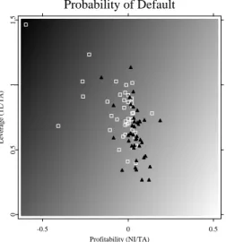
corresponds to different score values f. The darker the area, the higher the score and the greater is the probability of default. Most successful companies lying in the bright area have positive profitability and a reasonable leverage TL/TA of around 0.4, which makes economic sense.

(16)

1.5 Computational results Probability of Default -0.5 0 0.5 Profitability (NI/TA) 0 0.5 1 1.5 Leverage (TL/TA)

Figure 1.4: Ratings of companies in two dimensions. The case of a low com-plexity of classifier functions, the radial basis is 100Σ1/2_{, the} capac-ity is fixed atC= 1.

STFsvm01.xpl

classifier functions (the anisotropic radial basis is 100Σ1/2_{) with the capacity} fixed atC= 1. The discriminating rule in this case can be approximated by a linear combination of predictors and is similar to that suggested by discriminant analysis, although the coefficients of the predictors may be different.

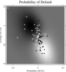
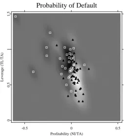
If the complexity of classifying functions increases (the radial basis goes down to 2Σ1/2_{) as illustrated in Figure 1.5, we get a more detailed picture. Now the} areas of successful and failing companies become localized. If the radial basis is decreased further down to 0.5Σ1/2 (Figure 1.6), the SVM will try to track each observation. The complexity in this case is too high for the given data set.

Figure 1.7 demonstrates the effects of high capacities (C= 300) on the classi-fication results. As capacity is growing, the SVM localizes only one cluster of successful companies. The area outside this cluster is associated with approxi-mately equally high score values.

(17)

Probability of Default -0.5 0 0.5 Profitability (NI/TA) 0 0.5 1 1.5 Leverage (TL/TA)

Figure 1.5: Ratings of companies in two dimensions. The case of an aver-age complexity of classifier functions, the radial basis is 2Σ1/2_{, the} capacity is fixed atC= 1.

STFsvm02.xpl

Thus, besides estimating the scores for companies the SVM also managed to learn that there always exists a cluster of successful companies, while the cluster for bankrupt companies vanishes when the capacity is high, i.e. a company must possess certain characteristics in order to be successful and failing companies can be located elsewhere. This result was obtained without using any additional knowledge besides that contained in the training set.

The calibration of the model or estimation of the mapping f → PD can be illustrated by the following example (the SVM with the radial basis 2Σ1/2 and capacity C = 1 will be applied). We can set three rating grades: safe, neutral and risky which correspond to the values of the score f < −0.0115, −0.0115 < f < 0.0115 and f > 0.0115, respectively, and calculate the to-tal number of companies and the number of failing companies in each of the three groups. If the training set were representative of the whole population of companies, the ratio of failing to all companies in a group would give the

(18)

1.5 Computational results Probability of Default -0.5 0 0.5 Profitability (NI/TA) 0 0.5 1 1.5 Leverage (TL/TA)

Figure 1.6: Ratings of companies in two dimensions. The case of an excessively high complexity of classifier functions, the radial basis is 0.5Σ1/2_, the capacity is fixed atC= 1.

STFsvm03.xpl

estimated probability of default. Figure 1.8 shows the power (Lorenz) curve (Lorenz, 1905) – the cumulative default rate as a function of the percentile of companies sorted according to their score – for the training set of compa-nies. For the abovementioned three rating grades we derive PDsafe = 0.24, PDneutral= 0.50 and PDrisky = 0.76.

If a sufficient number of observations is available, the model can also be cali-brated for finer rating grades such as AAA or BB by adjusting the score values separating the groups of companies so that the estimated default probabilities within each group equal to those of the corresponding rating grades. Note, that we are calibrating the model on the grid determined by grad(f) = 0 or grad ˆ(PD) = 0 and not on the orthogonal grid as in the Moody’s RiskCalc model. In other words, we do not make a restrictive assumption of an indepen-dent influence of predictors as in the latter model. This can be important since, for example, the same decrease in profitability will have different consequences

(19)

Probability of Default -0.5 0 0.5 Profitability (NI/TA) 0 0.5 1 1.5 Leverage (TL/TA)

Figure 1.7: Ratings of companies in two dimensions, the case of a high capacity (C= 300). The radial basis is fixed at 2Σ1/2_.

STFsvm04.xpl

for high and low leveraged firms.

For multidimensional classification the results can not be easily visualized. In this case we will use the cross-validation technique to compute the percentage of correct classifications and compare it with that for the discriminant analysis (DA). Note that both most widely used methods – the discriminant analysis and logit regression – choose only one significant at the 5% level predictor (NI/TA) when forward selection is used. Cross-validation has the following stages. One company is taken out of the sample and the SVM is trained on the remaining companies. Then the class of the out-of-the-sample company is evaluated by the SVM. This procedure is repeated for all the companies and the percentage of correct classifications is calculated.

The best percentage of correctly cross-validated companies (all available ratios were used as predictors) is higher for the SVM than for the discriminant analysis (62% vs. 60%). However, the difference is not significant at the 5% level. This indicates that the linear function might be considered as an optimal classifier

(20)

1.5 Computational results Power Curve 0 0.5 1 Percentile 0 0.5 1

Cumulative default rate

Figure 1.8: Power (Lorenz) curve (Lorenz, 1905) – the cumulative default rate as a function of the percentile of companies sorted according to their score – for the training set of companies. An SVM is applied with the radial basis 2Σ1/2 _{and capacity}_C_{= 1.}

STFsvmpc.xpl

for the number of observations in the data set we have. As for the direction vector of the separating hyperplane, it can be estimated differently by the SVM and DA without affecting much the accuracy since the correlation of underlying predictors is high.

Cluster center locations, as they were estimated using cluster analysis, are presented in Table 1.4. The results of the cluster analysis indicate that two clusters are likely to correspond to successful and failing companies. Note the substantial differences in the interest coverage ratios, NI/TA, EBIT/TA and TL/TA between the clusters.

(21)

Cluster {-1} {1} EBIT/TA 0.263 0.015 NI/TA 0.078 -0.027 EBIT/S 0.313 -0.040 EBIT/INT 13.223 1.012 TD/TA 0.200 0.379 TL/TA 0.549 0.752 SIZE 15.104 15.059 QA/CL 1.108 1.361 CASH/TA 0.047 0.030 WC/TA 0.126 0.083 CA/CL 1.879 1.813 STD/TD 0.144 0.061 S/TA 1.178 0.959 INV/COGS 0.173 0.155

Table 1.4: Cluster centre locations. There are 19 members in class{-1}– suc-cessful companies, and 65 members in class{1}– failing companies.

1.6 Conclusions

As we have shown, SVMs are capable of extracting information from real life economic data. Moreover, they give an opportunity to obtain the results not very obvious at first glance. They are easily adjusted with only few parame-ters. This makes them particularly well suited as an underlying technique for company rating and investment risk assessment methods applied by financial institutions.

SVMs are also based on very few restrictive assumptions and can reveal effects overlooked by many other methods. They have been able to produce accurate classification results in other areas and can become an option of choice for company rating. However, in order to create a practically valuable methodology one needs to combine an SVM with an extensive data set of companies and turn to alternative formulations of SVMs better suited for processing large data sets. Overall, we have a valuable tool for company rating that can answer the requirements of the new capital regulations.

(22)

Bibliography

Altman, E., (1968). Financial Ratios, Discriminant Analysis and the Prediction of Corporate Bankruptcy,The Journal of Finance, September: 589-609. Altman, E., Haldeman, R. and Narayanan, P., (1977). ZETA Analysis: a New

Model to Identify Bankruptcy Risk of Corporations, Journal of Banking and Finance, June: 29-54.

Basel Committee on Banking Supervision (2003). The New Basel Capital Ac-cord, third consultative paper,http://www.bis.org/bcbs/cp3full.pdf. Beaver, W., (1966). Financial Ratios as Predictors of Failures. Empirical

Re-search in Accounting: Selected Studies, Journal of Accounting Research, supplement to vol. 5: 71-111.

Damodaran, A., (2002).Investment Valuation, second ed., John Wiley & Sons, New York, NY.

Deakin, E., (1972). A Discriminant Analysis of Predictors of Business Failure,

Journal of Accounting Research, Spring: 167-179.

Dev, S., (1974). Ratio Analysis and the Prediction of Company Failure in Ebits, Credits, Finance and Profits, ed. H.C. Edy and B.S. Yamey, Sweet and Maxwell, London: 61-74.

Dimitras, A., Slowinski, R., Susmaga, R. and Zopounidis, C., (1999). Business Failure Prediction Using Rough Sets, European Journal of Operational Research, number 114: 263-280.

EUNITE, (2001). Electricity load forecast competition of the EUro-pean Network on Intelligent TEchnologies for Smart Adaptive Systems,

http://neuron.tuke.sk/competition/.

Falkenstein, E., (2000). RiskCalc for Private Companies: Moody’s Default Model, Moody’s Investors Service.

(23)

Fitzpatrick, P., (2000). A Comparison of the Ratios of Successful Industrial Enterprises with Those of Failed Companies, The Accounting Publishing Company.

Frydman, H., Altman, E. and Kao, D.-L., (1985). Introducing Recursive Par-titioning for Financial Classification: The Case of Financial Distress,The Journal of Finance,40_{: 269-291.}

F¨user, K., (2002). Basel II – was muß der Mittelstand tun?,

http://www.ey.com/global/download.nsf/Germany/Mittelstandsrating/

$file/Mittelstandsrating.pdf.

H¨ardle, W. and Simar, L. (2003). Applied Multivariate Statistical Analysis, Springer Verlag.

Gale, D., Kuhn, H.W. and Tucker, A.W., (1951). Linear Programming and the Theory of Games,Activity Analysis of Production and Allocation, ed. T.C. Koopmans, John Wiley & Sons, New York, NY: 317-329.

Lorenz, M.O., (1905). Methods for Measuring the Concentration of Wealth,

Journal of American Statistical Association,9_{: 209-219.}

Martin, D., (1977). Early Warning of Bank Failure: A Logit Regression Ap-proach,Journal of Banking and Finance, number 1: 249-276.

Mercer, J., (1909). Functions of Positive and Negative Type and Their Con-nection with the Theory of Integral Equations,Philosophical Transactions of the Royal Society of London,209_{: 415-446.}

Merton, R., (1974). On the Pricing of Corporate Debt: The Risk Structure of Interest Rates,The Journal of Finance, 29_{: 449-470.}

Ohlson, J., (1980). Financial Ratios and the Probabilistic Prediction of Bank-ruptcy,Journal of Accounting Research, Spring: 109-131.

Ramser, J. and Foster, L., (1931). A Demonstration of Ratio Analysis. Bul-letin No. 40, University of Illinois, Bureau of Business Research, Urbana, Illinois.

Division of Corporate Finance of the Securities and Exchange Com-mission, (2004). Standard industrial classification (SIC) code list,

http://www.sec.gov/info/edgar/siccodes.htm.

Securities and Exchange Commission, (2004). Archive of historical documents,

(24)

Bibliography

Tam, K. and Kiang, M., (1992). Managerial Application of Neural Networks: the Case of Bank Failure Prediction,Management Science, 38_{: 926-947.}

Tikhonov, A.N. and Arsenin, V.Y., (1977). Solution of Ill-posed Problems, W.H. Winston, Washington, DC.

Vapnik, V., (1995).The Nature of Statistical Learning Theory, Springer Verlag, New York, NY.

Wiginton, J., (1980). A Note on the Comparison of Logit and Discriminant Models of Consumer Credit Behaviour,Journal of Financial and Quanti-tative Analysis,15_{: 757-770.}

Wilcox, A., (1971). A Simple Theory of Financial Ratios as Predictors of Failure,Journal of Accounting Research: 389-395.

Winakor, A. and Smith, R., (1935).Changes in the Financial Structure of Un-successful Industrial Corporations. Bulletin No. 51, University of Illinois, Bureau of Business Research, Urbana, Illinois.

Zavgren, C., (1983). The Prediction of Corporate Failure: The State of the Art,Journal of Accounting Literature, number 2: 1-38.

Zmijewski, M., (1984). Methodological Issues Related to the Estimation of Financial Distress Prediction Models,Journal of Accounting Research,20_:

(25)