Classifying Imbalanced Multi-modal Sensor Data
for Human Activity Recognition in a Smart Home
using Deep Learning
Ali A. AlaniDepartment of Computer Science University of Diyala
Diyala, Iraq
Georgina Cosma Department of Computer Science
Loughborough University Loughborough, UK [email protected]
Aboozar Taherkhani School of Science and Informatics
De Montfort University Leicester, UK
Abstract— In smart homes, data generated from real-time sensors for human activity recognition is complex, noisy and imbalanced. It is a significant challenge to create machine learning models that can classify activities which are not as commonly occurring as other activities. Machine learning models designed to classify imbalanced data are biased towards learning the more commonly occurring classes. Such learning bias occurs naturally, since the models better learn classes which contain more records. This paper examines whether fusing real-world imbalanced multi-modal sensor data improves classification results as opposed to using unimodal data; and compares deep learning approaches to dealing with imbalanced multi-modal sensor data when using various resampling methods and deep learning models. Experiments were carried out using a large multi-modal sensor dataset generated from the Sensor Platform for HEalthcare in a Residential Environment (SPHERE). The data comprises 16104 samples, where each sample comprises 5608 features and belongs to one of 20 activities (classes). Experimental results using SPHERE demonstrate the challenges of dealing with imbalanced multi-modal data and highlight the importance of having a suitable number of samples within each class for sufficiently training and testing deep learning models. Furthermore, the results revealed that when fusing the data and using the Synthetic Minority Oversampling Technique (SMOTE) to correct class imbalance, CNN-LSTM achieved the highest classification accuracy of 93.67% followed by CNN, 93.55%, and LSTM, i.e. 92.98%.
Keywords—Human Activity Recognition, imbalanced data, multi-modal data, multi-sensor data, Deep Learning
I. INTRODUCTION
Human Activity Recognition (HAR) in smart homes is receiving increasing attention due to a wide range of potential applications, including physical activity recognition and intelligent assistance for elderly people and people with cognitive disorders [1]. In smart homes, data from various sensors may be fused to create models that recognise the activities of residents. Activity recognition models can provide information which can aid those making healthcare related decisions about patients, and those who are monitoring vulnerable patients. For example, human activity recognition models can be used to classify data and alert carers about falls, unordinary behaviour, or about certain activities. Additionally, the models can analyse different behaviours for detecting strokes, eating behaviour, and tracking whether people are taking prescribed medication [2]. An approach to HAR is based on a sliding window procedure, where a fixed length analysis window is shifted along the signal sequence for frame extraction [3]. Pre-processing transforms raw signal data into feature vectors,
which are then utilised to build machine learning models. Successful HAR relies on the design of appropriate feature representations of the sensor data, and the design of suitable machine learning methods [3]. Conventional machine learning methods that have been applied to the task of HAR include Naive Bayes and SVMs [4]. Deep Neural Networks (DNNs) such as Convolutional Neural Networks (CNN), and Recurrent Neural Networks (RNN) have achieved considerable performance across various applications and outperformed many conventional methods, particularly for computer vision and image classification tasks. Recently, hybrids of Long-Short-Term Memory (LSTMs) recurrent neural networks (that include a memory to model temporal dependencies in time series problems) and CNNs have been shown to provide state-of-the-art results on challenging activity recognition tasks with little or no feature engineering when modelling temporal information [5]. The problem encountered by online system applications that utilise Deep Learning (DL)-based approaches is that some classes have a much higher number of samples than other classes. This is known as the class imbalance problem. Processing of imbalanced data is one of the biggest challenges in data mining and machine learning (ML), and this problem occurs when some classes in the dataset have a significantly higher number of samples than other classes [6]. The class that overwhelms the other classes is called the majority class while the other classes are the minority classes. Class imbalance can be an intrinsic property in datasets or it can occur due to limitations in obtaining the data attributed to cost, privacy or due to limited data available. Many applications such as medical diagnosis, and fraud detection suffer from limited or imbalanced data [7].
The class imbalance problem can decrease the performance of ML models, as the overall model accuracy can be biased to the majority class, which can lead to misclassifying the minority class samples or furthermore treat data in minority classes as noisy data. Methods of dealing with the class imbalance problem are well studied for classical ML models and these methods can be divided into two main approaches [6]. The first approach concerns the use of data-level methods (such as data resampling methods) that aim to solve the class imbalance problem by changing the class distribution in the training set. The second approach relates to the classifier-level and it is called the algorithmic level method. In this method, the class distribution in the training set is unchanged, but it utilises the formulation of the learning algorithms by introducing different weights to misclassification examples from different classes [6]. However, this method is not generic and requires careful parameter selection [7].
This paper proposes a DL framework for the classification of daily living human activities using the Sensor Platform for HEalthcare in a Residential Environment (SPHERE) dataset which contains naturally imbalanced multi-modal data generated from different sensors installed in a smart home [8]. Various methods to deal with imbalance are explored when embedded into three DL techniques namely, the CNN, LSTM, and a hybrid CNN-LSTM which combines both models into one unified architecture, and these methods are compared in terms of classification performance. The paper is structured as follows: Section II explores related work, Section III describes the proposed approach, Section IV discusses experimental results, and Section V provides the conclusion and future work.
II. RELATED WORK
An accurate classification method of user activities allows the effective understanding of user habits and monitoring their health conditions. Existing approaches to current home monitoring systems often include custom-fit environmental, physiological and vision sensors, such as those utilised by the SPHERE project [8]. Depth sensors and wearable sensors have been used individually for human action recognition. However, simultaneous utilisation of both depth and wearable inertial sensors for human action recognition are less common. The automatic feature extraction and representation abilities of DL methods have become an emerging area of research in human activity recognition. Via their multi-layered architecture, DL methods can construct low level to high level representational features in sensor data hierarchically. Vella et al. [9] used two different CNN architectures namely Deep Net 1 and Deep Net 2, and compared these with a baseline multilayer perceptron (MLP) using the SPHERE dataset. In this work, the authors merged some classes to macro labels to have classes with more samples and more generic labels as a strategy to dealing with imbalanced classes. Their results show that the CNN outperformed the baseline MLP.
Cipolla et al. [10] present a system based on the deep LSTM network architecture to classify actions performed in an indoor environment using the SPHERE dataset. In order to deal with imbalanced classes in the dataset and to increase the training accuracy, they derived a set of generic labels using the original ones. In this context all the transition labels were clustered together in a simple label transition (for example the classes related to the ‘walking’ class were merged together into a single class), and this approach resulted in 83.2% classification accuracy.
Li et al. [11] proposed a hybrid CNN and LSTM for concurrent human activity recognition. Their proposed multi-sensor model recognises whether an activity occurs. Zhao et al. proposed a CNN and bidirectional LSTM for health monitoring by using various sensor modalities in order to model the temporal and sequential structure of data [12]. However, the combination architectures led to increased computation time and complexity, making these architectures unsuitable for real-time tasks. Other DL fusion methods were developed for human activity recognition by integrating DL methods and handcrafted feature techniques. Ravi et al., proposed the fusion of handcrafted features and a CNN for human activity recognition using mobile phone and wearable sensors [4]. Alzantot et al., to solve the problem of limited samples of training data, proposed an LSTM fused with a mixture density network to generate new samples
from sensor data for human activity recognition [13]. However, the high number of learning parameters of CNNs may increase the computation cost for real-time implementation.
III. PROPOSED APPROACHES AND EXPERIMENTS
This section describes the architecture of the CNN, LSTM, and CNN-LSTM algorithms which were designed for experiments using the SPHERE dataset, the resampling methods which were adopted for dealing with data imbalance. It provides a description of the SPHERE dataset. This section also presents the evaluation measures adopted for comparing the performance of the three deep learning models.
A. Convolutional Neural Network (CNN)
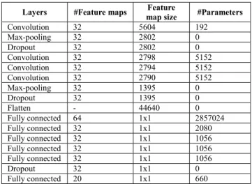
The CNN model used in the experiments has 4 convolution layers, each with a kernel size of 5 and a Rectified Linear Units (ReLU) activation function, 5 fully connected layers with the ReLU activation function, 2 max-pooling layers, 3 dropout regularization layers which have been configured to randomly exclude 0.2 of neurons to reduce over fitting. Finally, the model ends with the output layer, which contains 20 neurons for the 20 classes with a Softmax activation function to present the final classification result. All layers and their parameters are described in TABLE I. In order to improve the network training, weights were initialised by effectively preselecting the initial position of the model parameters with respect to the loss function to optimize.
The CNN network architecture uses uniform He initialization (he_uniform) for all ReLU layers and the uniform Xavier initialization (glorot_uniform) for the output Softmax layer to effectively generalize the logistic function for multiple inputs. Also, L2 regularization is used to penalise weights with large magnitudes, by minimizing their L2 norm. It uses a hyper parameter λ = 0.0001 to specify the relative importance of minimizing the norm compared to minimizing the loss on the training set. The proposed CNN model is trained in a fully supervised way. It backpropagates the gradients from the output Softmax layer to the convolutional layers.
TABLE I. CNN STRUCTURE
Layers #Feature maps map size Feature #Parameters
Convolution 32 5604 192 Max-pooling 32 2802 0 Dropout 32 2802 0 Convolution 32 2798 5152 Convolution 32 2794 5152 Convolution 32 2790 5152 Max-pooling 32 1395 0 Dropout 32 1395 0 Flatten - 44640 0 Fully connected 64 1x1 2857024 Fully connected 32 1x1 2080 Fully connected 32 1x1 1056 Fully connected 32 1x1 1056 Fully connected 32 1x1 1056 Dropout 32 1x1 0 Fully connected 20 1x1 660
B. Long Short-term Memory (LSTM)
The proposed LSTM architecture uses 3 layers, 2 dropout layers and a final layer which is the output layer for prediction. The first layer has size 5608 that contains 32 feature maps and a Rectified Linear Unit (ReLU) activation function. This layer represents the LSTM input layer. Next, is a regularization layer called Dropout. It is configured to randomly exclude 0.2 of neurons to reduce overfitting. This layer is followed by the second layer that contains 64 feature maps and a ReLU activation function. Next, is another regularization layer which randomly excludes 0.2 of neurons and this layer is followed by the final layer with 128 feature maps and a ReLU activation function. The final layer is the output layer added for prediction. This layer uses Softmax as the activation function. The proposed LSTM architecture and its parameters are described in TABLE II.
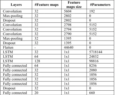
C. Hybrid CNN and LSTM Architecture (CNN-LSTM) A CNN-LSTM architecture has two sub-models, the CNN model on the front end for feature extraction, and an LSTM model for interpreting the features across time steps with dense and Softmax layers on the output. The proposed CNN-LSTM model comprises 4 convolutional layers, 2 pooling layers, 3 dropouts, 3 LSTM layers, 5 fully connected layers, and an output layer. The 5 fully connected layers are used to interpret the features extracted by the LSTM hidden layer. The output layer is obtained from a Softmax layer (a dense layer with a Softmax activation function), and it yields a probability distribution over classes. All the layers and their parameters are described in TABLE III.
TABLE II. LSTM STRUCTURE
Layers #Feature maps Feature map size #Parameters
LSTM 32 1x1 722048 Dropout 32 1x1 0 LSTM 64 1x1 24832 Dropout 64 1x1 0 LSTM 128 1x1 98816 Fully connected 20 1x1 2580 TABLE III. CNN-LSTM STRUCTURE
Layers #Feature maps maps size Feature #Parameters
Convolution 32 5604 192 Max-pooling 32 2802 0 Dropout 32 2802 0 Convolution 32 2798 5152 Convolution 32 2794 5152 Convolution 32 2790 5152 Max-pooling 32 1395 0 Dropout 32 1395 0 Flatten - 44640 0 LSTM 32 1x1 5718144 LSTM 64 1x1 24832 LSTM 128 1x1 98816 Fully connected 64 1x1 8256 Fully connected 32 1x1 2080 Fully connected 32 1x1 1056 Fully connected 32 1x1 1056 Fully connected 32 1x1 1056 Dropout 32 1x1 0 Fully connected 20 1x1 660
D. Methods for dealing with imbalanced data
This paper focuses on data level methods and hence using resampling methods to handle the problem of data imbalance in different classes, which concerns adjusting the prior distribution for the minority and majority classes. The resampling techniques fall into two groups (oversampling and undersampling) and these methods are used to balance the class distribution. Oversampling is a widely used method for creating synthetic samples from minority samples. The basic version of it is called random minority oversampling [6], which randomly duplicates samples from the minority classes. SMOTE (Synthetic Minority Oversampling Technique) [14] is an advanced sampling method that aims to overcome the class imbalance problem by artificially creating samples via the interpolation of neighbouring data points. Another type of oversampling method involves using data pre-processing methods to perform more informed oversampling. For example in [15], the authors firstly cluster the dataset and then oversample each cluster separately. An oversampling approach specific to neural networks optimised with stochastic gradient descent is class-aware sampling [16]. The main idea is to ensure uniform class distribution of each mini-batch, and to control the selection of examples from each class. Oversampling can increase classification performance effectively, however since it increases the number of samples of the minority class, it also increases the training time of the model. Undersampling is a resampling method for dealing with imbalanced datasets. Undersampling removes samples randomly from the majority classes until the dataset is balanced. A significant disadvantage of this method is that by removing samples from the majority classes, important information may be lost [6].
E. Dataset Description
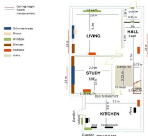
The SPHERE dataset for activity recognition, comprises data for making predictions from video, accelerometer and environmental sensors [8]. SPHERE consists of 20 different classes along with their corresponding labels. The labels are shown in the first column of TABLE VII. The SPHERE dataset was generated from 3 different sensors, the accelerometer worn by a participant, data collected from Passive InfraRed (PIR) sensors and 2D and 3D data obtained from three cameras. The obtained training data contains ten sets of sequences of recorded data with a length of ten minutes. The SPHERE home has a two floors the ground floor and the first floor as illustrated in Figs. 1 and 2 respectively [8]. The first floor contains three RGB-Depth cameras installed in the living room, hallway, and kitchen, and nine PIR sensors are located in the hall, kitchen, bath, bedroom 1, bedroom 2, living, toilet, study, and stairs. The dataset description available in [8] [3].
F. Pre-processing
In this paper, the goal is to identify 20 different human activities from accelerometer and RGB-D camera data as well as passive environmental sensor (PIR) data. However, classification algorithms cannot be directly applied to raw time-series accelerometer and camera data, and for this reason feature engineering was carried out on the SPHERE data. Initially the sensor data was divided into windows, where each window is a one-second time resolution in length and different features are extracted for all windows. This resulted in 14 extracted features for each time-series window.
These features are: mean value, standard deviation, minimum value, standard error of the mean (sem), the first central moment (deviation from mean), interquartile range (IQR), Median Absolute Deviation (MAD), median, maximum value, variance, skewness, the energy of the signal, kurtosis, and vector norm. Additionally, the first discrete difference of each time series for the fourteen features is calculated by (1).
x[n] = x[n +1] - x[n] 1
where x[n] is the time series value at time n. Moreover, extra features are extracted from the video data. These are the width and height difference from top left and bottom right coordinators and their ratio; the max, min and median of the distance between these two points. Furthermore, 28 extra features are extracted from the accelerometer data such as the correlation between x and y, x and z, correlation between y and z, Signal-Magnitude Area, entropy, the number of zero-crossing, etc.
The total number of extracted features was 1402 for each time window and the number of samples after removing all the time windows which did not have annotations was 16104-time windows. In order to recognise the activity of a participant in each time window the features related to four-time windows are used due to these windows contain useful information about the activity in the current time window, and these windows are: the information in the current time window, the information that exists in the two previous time windows and the information in the time window next to the current time window, these four-time windows can help to derive a more accurate recognition of the activity of a participant at the current time windows. Therefore, features related to the two lagged windows and the window next to the current window are combined to construct a feature vector with a length of 1402 x 4 = 5608 features for each activity. From 16104 samples in the dataset, a total of 11272 samples that represent 70% from the dataset were randomly extracted and considered as the training set, and a total of 4832 samples that represent 30% from the dataset were randomly extracted and considered as the training set samples (see TABLE IV). The SPHERE dataset contains twenty different classes as shown in Fig. 3, and these classes were used to recognize the activity of a participant at one-second intervals.
Fig. 1. Ground floor plan of the SPHERE smart house [8].
Fig. 2. First floor plan of the SPHERE smart house [8]. TABLE IV. CHARACTERISTICS OF THE SPHERE DATASET Dataset Labels Features vector Total of Samples (16104)
Training 70% Testing 30%
SPHERE 20 (5608, 1) 11272 4832
Fig. 3. Number of training and testing samples in each class. (A1: ascent stairs, A2: Descent stairs, A3: Jump, A4: walk with load, A5: Walk, A6: Bending, A7: Kneeling, A8: Lying, A9: Sitting, A10: Squatting, A11: standing, A12: stand-to-bend, A13: kneel-to-stand, A14: lie-to-sit, A15: sit-to-lie, A16: sit-to-stand, A17: stand-to-kneel, A18: stand-to-sit, A19: bend-to-stand, A20: turn)
G. Evaluation Measures
The classification accuracy is used to evaluate the performance of the DL approaches. Accuracy (A), is the total number of samples correctly classified (TCC) divided by the total number of samples (T), multiplied by 100 to turn it into a percentage. The formula for calculating A is shown in (2).
∗ 100 2
The accuracy can be calculated for a class using (3).
∗ 100 3
Where TCCc is the number of the correct assignments which
are from the class c, Tc is the total numbers of samples
which are belong to the class c. The calculated value is multiplied by 100 to get the percentage of the accuracy.
IV. RESULTS AND DISCUSSION
This section describes the results of the experiments when using the CNN, LSTM and CNN-LSTM architectures. Experiments were performed using Python, mainly taking
advantage of the Tensorflow and Keras Python DL libraries. In the first pre-processing step, the raw data was standardised by removing their mean and scaling it to unit variance. The training process for all three DL models are based on the back-propagation algorithm with the stochastic gradient descent method, and the categorical cross entropy loss function is used as the cost function, also the Adam optimizer function is used as the optimization function, these settings were chosen experimentally as the best options. The results of the experiments when using the three models are described in the following subsections.
A. Results when using unimodal data for HAR
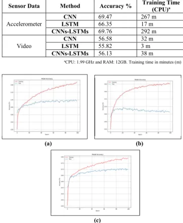
The performance of the three models (CNN, LSTM and CNN-LSTM) using the individual modalities of accelerometer and video is shown in TABLE V. The training data is split into batches, each containing 32 training samples. There are 3528 neurons in the input layers when training the models using the accelerometer sensor data, and 372 neurons in the input layers when training the models using video data. There are 20 neurons in the output layers of all three proposed models. Learning is continued for 100 learning epochs. As shown in TABLE V. , the performance obtained by using the accelerometer data is better than the performance achieved when using the video data for all three DL models. Highest recognition accuracy was obtained by CNN-LSTM, 69.76%, which is higher than those obtained by the CNN, i.e. 69.47%, and LSTM, i.e. 66.35%, when using the accelerometer data.
In Fig. 4, the accuracy of the proposed models is shown during different learning epochs by accelerometer data. Fig. 4(a) shows the accuracy of CNN on the training set is increased during all learning epochs. However, the accuracy on the testing set has not improved after epoch 60 and the model begins overfitting. Fig. 4 (b) shows the accuracy of the LSTM on the training set is increased during all learning epochs. However, the accuracy of the testing set has not improved after epoch 20 and the model begins overfitting. Finally, Fig. 4 (c) shows the accuracy of CNN-LSTM on the training set is increased during all the learning epochs. However, the accuracy on the testing set has not improved after epoch 95 and overfitting begins to occur.
B. Results when using multi-modal data for HAR
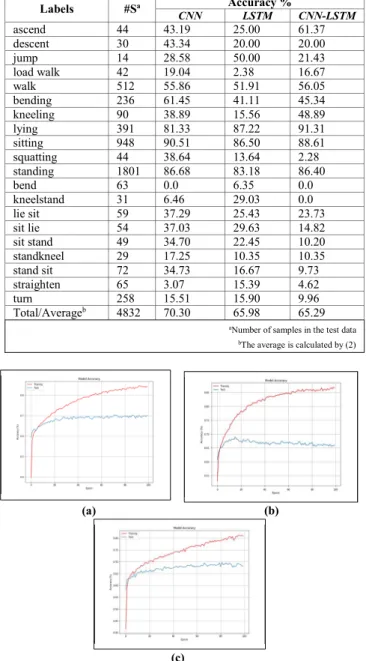
In the second set of experiments, the proposed classifiers are trained by combining all various modalities (accelerometer, video, PIR). TABLE VI presents the results when using the CNN, LSTM and CNN-LSTM architectures applied to the SPHERE dataset. As expected, combining several modalities increases the recognition performance because, in general, the features extracted from one modality complement the drawbacks of the features extracted from other modalities. The results show that the CNN architecture achieved 70.30% accuracy, which was higher than the performance obtained by the LSTM and CNN-LSTM architectures, i.e. 65.98% and 68.29%, respectively.
The accuracy of all 20 classes is shown in TABLE VII. The number of training and testing samples across the classes varies considerably. For example, there are 14 testing samples labelled by ‘jump’ class and 1801 testing samples labelled as ‘standing’ class. The relatively high numbers of samples in classes such as ‘standing’, ‘laying’ and ‘sitting’ cause these classes have a high accuracy in all proposed models.
TABLE V. CNN, LSTM, AND CNN-LSTM CLASSIFICATION RESULTS USING ACCELEROMETER DATA (UNIMODAL DATA)
Sensor Data Method Accuracy % Training Time (CPU)a Accelerometer CNN 69.47 267 m LSTM 66.35 17 m CNNs-LSTMs 69.76 292 m Video CNN 56.58 32 m LSTM 55.82 3 m CNNs-LSTMs 56.13 38 m
aCPU: 1.99 GHz and RAM: 12GB. Training time in minutes (m)
Fig. 4. Accelerometer data: Training and testing accuracy of (a) CNN model, (b) LSTM model, and (c) CNN-LSTM model.
For instance, the accuracy of the ‘standing’ class was 86.68%, 83.13%, and 86.40% for CNN, LSTM and CNN-LSTM, respectively, which are high accuracy values when compared to the accuracy values obtained for the other classes. The results highlight the impact of class imbalance on classification performance. Therefore, finding a strategy to deal with the impact of class imbalance on classification performance is required. Oversampling and undersampling techniques are used to address this problem. Importantly, Fig. 5, depicts the model accuracy when adopting CNN, LSTM and CNN-LSTM respectively. Fig. 5, shows that the overall classification performance of the CNN architecture is higher than the LSTM and CNN-LSTM architectures. C. Results when applying oversampling and undersampling
The baseline performance results mentioned in the previous subsection were obtained by training the proposed models with no data sampling. The results revealed that the imbalanced distribution of training data in different classes has a significant impact on the performance of the models. This subsection describes the results when using resampling methods to handle the problem of imbalance in the number of samples across the different classes in the SPHERE dataset.
TABLE VI. CNN, LSTM AND CNN-LSTM RESULTS (MULTI-MODAL DATA, NO SAMPLING)
Method Accuracy % Training Time (GPU)a
CNN 70.30 11 m
LSTM 65.98 6 m
CNNs-LSTMs 68.29 19 m
aGPU: NVIDIA Tesla K80 and RAM: 12 GB.
(b) (a)
TABLE VII. CNN, LSTM AND CNN-LSTM ACCURACY ON THE TEST DATA (MULTI
-MODAL DATA, NO SAMPLING)
Labels #Sa Accuracy % CNN LSTM CNN-LSTM ascend 44 43.19 25.00 61.37 descent 30 43.34 20.00 20.00 jump 14 28.58 50.00 21.43 load walk 42 19.04 2.38 16.67 walk 512 55.86 51.91 56.05 bending 236 61.45 41.11 45.34 kneeling 90 38.89 15.56 48.89 lying 391 81.33 87.22 91.31 sitting 948 90.51 86.50 88.61 squatting 44 38.64 13.64 2.28 standing 1801 86.68 83.18 86.40 bend 63 0.0 6.35 0.0 kneelstand 31 6.46 29.03 0.0 lie sit 59 37.29 25.43 23.73 sit lie 54 37.03 29.63 14.82 sit stand 49 34.70 22.45 10.20 standkneel 29 17.25 10.35 10.35 stand sit 72 34.73 16.67 9.73 straighten 65 3.07 15.39 4.62 turn 258 15.51 15.90 9.96 Total/Averageb 4832 70.30 65.98 65.29
aNumber of samples in the test data bThe average is calculated by (2)
Fig. 5. Training and testing accuracy of (a) CNN model, (b) LSTM model, and (c) CNN–LSTM model (multi-modal data, no sampling).
The resampling methods construct a balanced training data set and adjust the prior distribution for minority and majority classes.
a) Oversampling: Twooversampling techniques were used to randomly duplicate samples in the minority class in order to balance the dataset. The Random Minority Oversampling [6], and the Synthetic Minority Oversampling TEchnique (SMOTE) [14] methods were utilised in the experiments. TABLE VIII. presents the results when using the CNN, LSTM, and CNN-LSTM architectures on the SPHERE dataset after random minority oversampling and SMOTE are applied to the data. Additionally, the per-class accuracy is reported in TABLE IX. There are 5608 neurons in the input layers and there are 20 neurons in the output layers of all the three proposed models. In these experiments, 10 training epochs over the training data were completed as these were sufficient for training the models without overfitting. The experimental results show that
when the SMOTE resampling method was applied, the CNN, LSTM, and CNN-LSTM achieved higher classification performance, compared to when the random minority oversampling method was used. In Fig. 6, the accuracy of the deep learning models after applying the random minority oversampling method are shown during different learning epochs. As it can be observed from Fig. 6, the accuracy of the models on the training and testing sets increases during all learning epochs, and the results show that a higher number of training epochs can improve the performance of the network.
The accuracy of the proposed models after applying the SMOTE method are shown during different learning epochs reported in Fig. 7. As it can be observed, the accuracy of the models on the training and testing sets increases for all learning epochs.
b) Undersampling: was used for adjusting the balance of samples across classed in the SPHERE dataset. Undersampling randomly removed samples from majority classes until the dataset was balanced. TABLE X. presents the results when using the CNN, LSTM and CNN-LSTM architectures applied to the SPHERE dataset after undersampling. The experiment results show that the CNN achieved 29.37% accuracy, which was lower than the performance obtained by the LSTM and CNN-LSTM architectures achieved 37.94% and 30.85%, respectively. The accuracy per-class is reported in TABLE XI.
TABLE VIII. CNN, LSTM AND CNN-LSTM CLASSIFICATION RESULTS AFTER APPLYING OVERSAMPLING TECHNIQUES (MULTI-MODAL DATA)
Method Random Minority Oversampling Accuracy % Training Time (CPU) SMOTE Accuracy % Training Time (CPU) CNN 92.94 302 m 93.55 285 m LSTM 92.12 16 m 92.98 15 m CNNs-LSTMs 92.33 326 m 93.67 323 m
TABLE IX. CNN, LSTM AND CNN-LSTM ACCURACY ON THE TEST DATA AFTER APPLYING RANDOM MINORITY SAMPLING AND SMOTE
Activity #Sa Random minority oversampling SMOTE CNN LSTM LSTM CNN- CNN LSTM LSTM CNN-ascend 1841 100 99.30 100 100 99.46 100 descent 1795 100 100 100 100 100 100 jump 1852 100 98.33 100 100 99.03 100 load walk 1789 73.40 88.99 64.73 73.84 74.46 73.34 walk 1811 91.28 97.85 91.00 92.71 90.01 91.66 bending 1867 99.58 100 99.52 99.14 99.73 99.73 kneeling 1798 96.00 94.17 94.61 93.60 94.72 92.88 lying 1867 81.10 88.97 85.70 81.68 82.00 88.75 sitting 1779 100 100 100 100 100 99.83 squatting 1813 43.19 68.51 47.22 65.85 56.45 59.72 standing 1794 100 100 98.11 99 99.22 98.94 bend 1776 100 100 100 100 99.61 99.32 kneelstand 1858 100 84.61 100 100 99.89 99.52 lie sit 1830 100 99.35 100 100 97.92 100 sit lie 1772 100 97.01 98.42 99.15 98.76 98.48 sit stand 1824 100 100 100 99.89 100 99.62 standkneel 1809 99.62 100 100 100 99.94 99.28 stand sit 1833 99.35 98.59 96.46 98.75 99.18 99.07 straighten 1735 74.36 87.32 96.23 70.37 69.97 75.27 turn 1845 100 100 100 99.46 100 100 Total/ Averageb 36288 92.94 92.12 92.33 93.55 92.98 93.67
aNumber of samples in the test data bThe average is calculated by (2).
(b) (a)
The performance of the deep learning models after applying the undersampling method are shown in Fig. 8. As it can be observed, the undersampling technique resulted in overfitting, and the gap between training and testing performance increased with iterations. In conclusion, applying undersampling has discarded samples from the majority classes which were important samples for training the deep learning models, and this resulted in decreased performance across all deep learning models.
Fig. 6. Random minority oversampling accuracy of the proposed models for training and testing on multi-modal data. (a) CNN model, (b) LSTM model, and (c) CNN-LSTM model
Fig. 7. SMOTE accuracy of the proposed models for training and testing on multi-modal data, (a) CNN model, (b) LSTM model, and (c) CNN-LSTM model.
TABLE X. CNN, LSTM AND CNN-LSTM CLASSIFICATION RESULTS AFTER APPLYING UNDERSAMPLING (MULTI-MODAL DATA)
Methods Accuracy % Training Time (GPU)
CNN 29.37 0.75 m
LSTM 37.94 1 m
CNNs-LSTMs 30.85 1 m
TABLE XI. CNN, LSTM AND CNN-LSTM ACCURACY ON THE TEST DATA AFTER APPLYING UNDERSAMPLING (MULTI-MODAL DATA)
Labels #Sa Accuracy % CNN LSTM CNN-LSTM ascend 15 53.00 80.00 73.00 descent 16 56.00 81.00 38.00 jump 12 66.00 50.00 42.00 load walk 20 15.00 10.00 10.00 walk 18 16.00 11.00 6.00 bending 17 0.00 18.00 6.00 kneeling 14 43.00 50.00 57.00 lying 13 54.00 54.00 54.00 sitting 14 21.00 43.00 36.00 squatting 13 15.00 31.00 15.00 standing 13 15.00 23.00 15.00 bend 8 38.00 50.00 50.00 kneelstand 12 50.00 42.00 33.00 lie sit 10 40.00 60.00 40.00 sit lie 9 22.00 22.00 44.00 sit stand 18 33.00 28.00 28.00 standkneel 18 11.00 39.00 39.00 stand sit 17 0.00 24.00 18.00 straighten 11 9.00 27.00 9.00 turn 14 64.00 43.00 36.00 Total/Averageb 282 29.37 37.94 30.85
aNumber of samples in the test data bThe average is calculated by (2).
Fig. 8. Undersamplingaccuracy of the deep learning models for training and testing data. (a) CNN model, (b) LSTM model, and (c) CNN-LSTM model (multi-modal data)
V. COMPARISON WITH STATE-OF-THE-ART METHODS The experiment results show that the performance achieved by the proposed models using all 20 activities (class) is much higher than the performance obtained in [9] and [10], when the authors merged some classes as a strategy to create classes with more samples. They gave the merged classes more generic labels to avoid the problem of imbalance classes. Vella et al. [9] used CNN and the best results achieved is 76%, and Cipolla et al. [10] used the LSTM and the best results achieved is 83.2%. A comparison results of the proposed methods and state-of-the-art methods specifically which were also applied to the SPHERE dataset are listed in TABLE XII.
In [3] the authors proposed and compared the performance of a CNN (which comprised two pairs of convolutional and max-pooling layers) and a Deep Belief Network for the task of human activity recognition using the SPHERE dataset, and their results show that the performance
(b) (a) (c) (b) (a) (c) (b) (a) (c)
TABLE XII. PERFORMANCE COMPARISON OF METHODS (MULTI-MODAL DATA)
Authors Methods #Classes #Epochs Accuracy
Taherkhani, et al. [3]
CNN 20 15 58.79
DBN 20 40 44.90
Result using raw data (Our approach) CNN 20 100 70.30 LSTMs 20 100 65.98 CNN-LSTM 20 100 68.29 Result with SMOTE (Our approach) CNN 20 10 93.55 LSTMs 20 10 92.98 CNN-LSTM 20 10 93.67
achieved by CNN, 58.79%, is much higher than the performance obtained by the DBN, 44.9%. The authors also highlighted the importance of having a large number of samples when training DL models. Additionally, when the authors trained the models using data from the four classes that had the highest number of samples, the DBN achieved 65.97% classification accuracy, whereas the CNN achieved 75.33% accuracy. However, a significant achievement is made by our proposed methods using CNN, LSTM and CNN-LSTM after applying the SMOTE resampling technique. CNN-LSTM, CNN, and LSTM reached the accuracies of 93.67%, 93.55% and 92.98%, respectively, when the SMOTE method was used. These findings demonstrate that having a suitable number of samples within each class can improve the generalization performance of DL models.
I. CONCLUSION
Activity recognition has recently gained a lot of interest and appears to be a promising approach in smart homes due to a wide range of potential applications, including intelligent assistance for elderly people and people with cognitive disorders. However, in smart homes, the data collected from real-time multi-modal sensor data is complex, noisy and imbalanced. To our knowledge, this is the first paper that looks at class imbalance and hybrid deep learning models on the data collected from multiple sensors SPHERE dataset.
In this paper, three different deep neural networks namely CNN, LSTM, and a hybrid CNN-LSTM have been designed and evaluated using data collected from multiple sensors observing everyday activities in a digital health care monitoring context. The objective of this research work was to examine whether fusing multi-sensor imbalanced data to create a multi-modal data improves classification results as opposed to unimodal datasets, and to compare various DL approaches to dealing with imbalanced sensor multi-modal data.
The experiment results reveal the challenges of dealing with imbalanced multi-modal data and highlight the importance of having a large number of samples within each class for sufficiently training and testing DL models. Furthermore, the results revealed the effectiveness of the SMOTE resampling method when applied to multi-modal sensor data. Future work includes performing further experiments with larger data obtained from real-world settings, and investigating algorithmic-based approaches to dealing with class imbalance.
ACKNOWLEDGMENT
Dr Cosma and Dr Taherkhani acknowledge the financial support of The Leverhulme Trust for the Research Project Grant RPG-2016-252 entitled Novel Approaches for Constructing Optimised Multi-modal Data Spaces.
R
EFERENCES[1] M. Jethanandani, et al, "Binary Relevance Model for Activity Recognition in Home Environment using Ambient Sensors," 2019 IEEE International Conference on Consumer Electronics - Taiwan (ICCE-TW), YILAN, Taiwan, pp. 1-2, 2019.
[2] G. A. Oguntala et al., "SmartWall: Novel RFID-Enabled Ambient Human Activity Recognition Using Machine Learning for Unobtrusive Health Monitoring," in IEEE Access, vol. 7, pp. 68022-68033, 2019.
[3] Taherkhani, A., Cosma, G., Alani, A.A. and McGinnity, T.M.. "Activity recognition from multi-modal sensor data using a deep convolutional neural network." In Science and Information Conference, pp. 203-218. Springer, Cham, 2018.
[4] D. Ravì, C. Wong, B. Lo and G. Yang, "A Deep Learning Approach to on-Node Sensor Data Analytics for Mobile or Wearable Devices," in IEEE Journal of Biomedical and Health Informatics, vol. 21, no. 1, pp. 56-64, Jan. 2017. [5] T. N. Sainath, et al , "Convolutional, Long Short-Term
Memory, fully connected Deep Neural Networks," 2015 IEEE International Conference on Acoustics, Speech and Signal Processing (ICASSP), Brisbane, QLD, pp. 4580-4584, 2015.
[6] Buda, M., Maki, A. and Mazurowski, M.A. "A systematic study of the class imbalance problem in convolutional neural networks." Neural Networks 106, pp. 249-259, 2018.
[7] S. Sukhanov, et al, "Combining SVMS for Classification on Class Imbalanced Data," 2018 IEEE Statistical Signal Processing Workshop (SSP), Freiburg, pp. 90-94, 2018. [8] Twomey, Niall, et al. "The SPHERE challenge: Activity
recognition with multimodal sensor data." arXiv preprint arXiv:1603.00797, 2016.
[9] Vella, Filippo, et al, "Classification of Indoor Actions through Deep Neural Networks," 2016 12th International Conference on Signal-Image Technology & Internet-Based Systems (SITIS), Naples, pp. 82-87, 2016. [10] Cipolla, E., Infantino, I., Maniscalco, U., Pilato, G. and
Vella, F. "Indoor actions classification through long short term memory neural networks." In International Conference on Image Analysis and Processing, pp. 435-444. Springer, Cham, 2017.
[11] Li, Xinyu, et al. "Concurrent activity recognition with multimodal CNN-LSTM structure." arXiv preprint arXiv:1702.01638, 2017.
[12] Zhao, R., Yan, R., Wang, J. and Mao, K.. "Learning to monitor machine health with convolutional bi-directional LSTM networks." Sensors 17, no. 2, pp. 273, 2017. [13] M. Alzantot, S. Chakraborty and M. Srivastava,
"SenseGen: A deep learning architecture for synthetic sensor data generation," 2017 IEEE International Conference on Pervasive Computing and Communications Workshops (PerCom Workshops), Kona, HI, pp. 188-193, 2017.
[14] Chawla, Nitesh V., et al. "SMOTE: synthetic minority over-sampling technique." Journal of artificial intelligence research 16, pp. 321-357, 2002 .
[15] Jo, Taeho, and Nathalie Japkowicz. "Class imbalances versus small disjuncts." ACM Sigkdd Explorations Newsletter 6, no. 1 pp. 40-49, 2004.
[16] Shen, Li, Zhouchen Lin, and Qingming Huang. "Relay backpropagation for effective learning of deep convolutional neural networks." In European conference on computer vision, pp. 467-482. Springer, Cham, 2016.