Geo-localization Refinement of Optical Satellite Images by Embedding Synthetic Aperture Radar Data in Novel Deep Learning Frameworks

(1)

Geo-localization Refinement of Optical Satellite Images

by Embedding Synthetic Aperture Radar Data in

Novel Deep Learning Frameworks

Dissertation

Zur Erlangung

des Doktorgrades der Naturwissenschaften (Dr. rer. nat.) des Fachbereichs Mathematik/Informatik

der Universität Osnabrück

Vorgelegt von

Nina Marie Merkle

Prüfer der Dissertation:

Prof. Dr. Peter Reinartz, Universität Osnabrück

Prof. Dr. habil. Stefan Hinz, Karlsruher Institut für Technologie

(2)

(3)

i

ABSTRACT

Every year, the number of applications relying on information extracted from high-resolution satellite imagery increases. In particular, the combined use of different data sources is rising steadily, for example to create high-resolution maps, to detect changes over time or to conduct image classification. In order to correctly fuse information from multiple data sources, the utilized images have to be precisely geometrically registered and have to exhibit a high absolute geo-localization accuracy. Due to the image acquisition process, optical satellite images commonly have an absolute geo-localization accuracy in the order of meters or tens of meters only. On the other hand, images captured by the high-resolution synthetic aperture radar satellite TerraSAR-X can achieve an absolute geo-localization accuracy within a few decimeters and therefore represent a reliable source for absolute geo-localization accuracy improvement of optical data. The main objective of this thesis is to address the challenge of image matching between high resolution optical and synthetic aperture radar (SAR) satellite imagery in order to improve the absolute geo-localization accuracy of the optical images. The different imaging properties of optical and SAR data pose a substantial challenge for a precise and accurate image matching, in particular for the handcrafted feature extraction stage common for traditional optical and SAR image matching methods. Therefore, a concept is required which is carefully tailored to the characteristics of optical and SAR imagery and is able to learn the identification and extraction of relevant features. Inspired by recent breakthroughs in the training of neural networks through deep learning techniques and the subsequent developments for automatic feature extraction and matching methods of single sensor images, two novel optical and SAR image matching methods are developed. Both methods pursue the goal of generating accurate and precise tie points by matching optical and SAR image patches. The foundation of these frameworks is a semi-automatic matching area selection method creating an optimal initialization for the matching approaches, by limiting the geometric differences of optical and SAR image pairs. The idea of the first approach is to eliminate the radiometric differences between the images trough an image-to-image translation with the help of generative adversarial networks and to realize the subsequent image matching through traditional algorithms. The second approach is an end-to-end method in which a Siamese neural network learns to automatically create tie points between image pairs through a targeted training. The geo-localization accuracy improvement of optical images is ultimately achieved by adjusting the corresponding optical sensor model parameters through the generated set of tie points.

The quality of the proposed methods is verified using an independent set of optical and SAR image pairs spread over Europe. Thereby, the focus is set on a quantitative and qualitative evaluation of the two tie point generation methods and their ability to generate reliable and accurate tie points. The results prove the potential of the developed concepts, but also reveal weaknesses such as the limited number of training and test data acquired by only one combination of optical and SAR sensor systems. Overall, the tie points generated by both deep learning-based concepts enable an absolute geo-localization improvement of optical images, outperforming state-of-the-art methods.

(4)

(5)

iii

ZUSAMMENFASSUNG

Aufgrund der steigenden Zahl an Anwendungen, die sich auf hochauflösenden Satellitendaten stützen, gewinnt auch die kombinierte Nutzung mehrerer Datenquellen immer mehr an Be-deutung. Beispielsweise können mit der Fusion mehrerer Datenquellen hochauflösende Karten erstellt oder Bildklassifikationen durchgeführt werden. Voraussetzung für eine korrekte Fu-sion von Informationen aus mehreren Datenquellen ist eine präzise Registrierung aller Bilder verbunden mit einer hohen Lagegenauigkeit der einzelnen Datenquellen. Aufgrund ihres Bildaufnahme-Verfahrens weisen optische Satellitenbilder in der Regel jedoch eine geringere Lagegenauigkeit im zweistelligen Meterbereich auf. Dagegen können Bilder des hochau-flösenden Radarsatelliten TerraSAR-X eine absolute Lagegenauigkeit innerhalb weniger Dezimeter erreichen und stellen somit eine zuverlässige Quelle zur Verbesserung der absoluten Lagegenauigkeit dar. Das Hauptziel dieser Arbeit ist die Verbesserung des Bild-Matchings zwischen hochauflösenden optischen und Synthetic Aperture Radar (SAR) Satellitenbildern, um damit die absolute Lagegenauigkeit von optischen Bildern zu verbessern.

Die unterschiedlichen Abbildungseigenschaften von optischen und SAR-Bildern stellen für die gängigen Methoden zur Bildregistrierung eine große Herausforderung dar, insbesondere für den Schritt der Merkmalsextraktion. Aus diesem Grund ist ein Verfahren erforder-lich, das auf die speziellen Eigenschaften von optischen und SAR-Bildern zugeschnitten ist und die Identifizierung und Extraktion von relevanten Merkmalen erlernen kann. In-spiriert durch die jüngsten Durchbrüche beim Training neuronaler Netze mit Hilfe von Deep Learning Techniken und den resultierenden Entwicklungen bei der automatischen Bild-Merkmalsextraktion und beim Bild-Matching, werden in dieser Arbeit zwei neuartige Verfahren für die Erzeugung von Verknüpfungspunkten zwischen optischen und SAR-Bildern vorgestellt. Das Ziel beider Bild-Matching Verfahren ist die Erzeugung präziser Verknüp-fungspunkte zwischen optischen und SAR-Bildpaaren. Für eine optimale Ausgangssituation des Bild-Matchings sorgt ein halbautomatisches Verfahren zur Auswahl der Matching-Gebiete. Hierdurch werden die geometrischen Unterschiede zwischen optischen und SAR-Bildpaaren auf ein Minimum reduziert. Die Idee der ersten Methode besteht darin, die radiometrischen Unterschiede zwischen den Bildpaaren durch Anwendung einer Bild-zu-Bild Transformation durch sogenannte „generative adversarial networks“ zu beseitigen und danach das eigentliche Bild-Matching durch traditionelle Methoden zu realisieren. Die zweite Methode ist ein „end-to-end“ Ansatz, bei dem ein siamesisches neuronales Netzwerk durch ein gezieltes Training lernt, automatisch Verknüpfungspunkte zwischen Bildpaaren zu erzeugen. Schließlich werden mit Hilfe der generierten Punkte die optischen Sensormodellparameter angepasst und somit die Lagegenauigkeiten der optischen Bilder verbessert.

Die Qualität der vorgeschlagenen Verfahren zur Bildregistrierung wird anhand voneinander unabhängiger und über ganz Europa verteilter optischer und SAR-Bildpaaren ausgewertet. Dabei liegt der Fokus auf einer sowohl quantitativen als auch qualitativen Auswertung der beiden Verfahren zur Generierung von Verknüpfungspunkten. Die Ergebnisse belegen das Potenzial der entwickelten Methoden, zeigen aber auch Schwächen wie beispielsweise die begrenzte Anzahl von Trainings- und Testdaten, erstellt aus den Bildern eines optischen bzw. SAR Sensors. Insgesamt ermöglichen die von beiden Verfahren erzeugten Verknüpfungspunkte eine Verbesserung der absoluten Lagegenauigkeit optischer Bilder und sind dabei genauer als State-of-the-Art Methoden.

(6)

(7)

1

Introduction

Contents

1.1 Motivation and Scope . . . 2

1.2 Scientific Relevance of the Topic . . . 2

1.3 Our Contributions and Focus of the Thesis . . . 4

(10)

2 1. Introduction

1.1 Motivation and Scope

In the last years, the technical advances in sensors systems and the increasing number of national and international space programs led to a strongly growing volume of remote sensing data. At the same time, the increased processing power and the development of new tools and algorithms boosted the applications of these data in terms of efficiency, reliability and robustness. In particular, the joint use of multi-modal data such as optical and synthetic aperture radar (SAR) images contain complementary information on objects on the Earth surface, which enriches the information conveyed by an object for several applications such as the generation of high-resolution maps for autonomous driving, the monitoring and modeling of changes over time for precision farming and urban planning. Despite the latest developments and technological advances, an accurate geo-referencing and co-registration step is still a prerequisite for the successful joint use of images acquired from different data sources. Very often, such steps are difficult to carry out with satisfactory precision in an unsupervised way, due to the intrinsic limitations in the sensors’ specific acquisition modes. The goal of this thesis is performing multi-modal image registration of high-resolution optical and SAR satellite images in order to enhance the absolute geo-localization accuracy of the former. To this end, deep learning techniques are utilized to develop two novel tie point generation methods, which enable an enhanced registration of optical and SAR image pairs and therefore a highly improved orthorectification of optical image data.

1.2 Scientific Relevance of the Topic

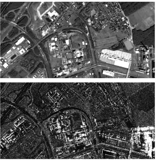
The collection of complementary information from aligned multi-modal image data enables a more detailed and more robust understanding of an image scene or specific object, and is important for several applications in the fields of medical imaging, computer vision or remote sensing [1–4]. In the particular case of optical and SAR satellites, the images acquired by these sensors exhibit different behavior (see example illustrated in Figure 1.1). These different and often complementary characteristics have been proven to be conducive for diverse applications in the field of remote sensing. More specific, several research studies investigated possibilities of their combined usage for tasks such as earthquake damage assessment of buildings [5], road network extraction [6], land cover classification [7], change detection [8], urban surface model generation [9–12] and stereogrammetric 3D analysis of urban areas [13]. However, optical and SAR satellite images are affected by acquisition related influences leading to local or global distortions, which lower the accuracy of the extracted information affecting in particular the absolute geo-localization accuracy of the optical images, thus hindering the use of optical images in any data fusion application. To overcome this fusion problem, the absolute geo-localization accuracy of optical images has to be improved beforehand. A common approach is the use of ground control points (GCPs) obtained from tedious in-situ GPS measurements or from very exact maps. The generation of GCPs is time consuming and expensive and therefore only available in a minority of cases. Another possibility is to align optical images to an image with a high absolute geo-localization accuracy. As images captured by the high-resolution SAR satellite TerraSAR-X can reach an absolute geo-localization accuracy within a few decimeters, or

(11)

1. Introduction 3

Figure 1.1: Illustration of an optical (top) and SAR image (bottom) covering the same area. Both images have a ground sampling distance of 1.25 m.

centimeters for specific targets [14], they represent a reliable source for the geo-localization accuracy improvement of optical images. Over the last years, different research studies investigated the geo-localization accuracy improvement of optical satellite images based on SAR reference data, achieving promising results [15–19]. These works rely on suitable image registration techniques, which are tailored to the problem of optical and SAR images matching. Due to the different acquisition concepts it is difficult to find identical features in both image modalities or reliable similarity measures. More precisely, the sideways-looking acquisition of SAR sensors causes typical geometric distortion effects (layover, foreshortening) and shadowing for 3D objects such as buildings or trees. These effects have a strong influence on the appearance of all objects above ground level. As a consequence, the boundary of an elevated object in a SAR image does not match the object boundary in the optical image, even if the imaging perspective is the same for both sensors. Additionally, the different wavelengths measured by the two sensors lead to different radiometric properties in the optical and SAR images. This is due to the fact that the response of an object depends on the

(12)

4 1. Introduction

signal properties (wavelength, polarization), the surface properties (roughness, randomness of local reflectors and reflectance properties) and sensor perspective. The same object may therefore appear with high intensity for one sensor and with low intensity in another. The multiplicative noise in SAR images (speckle) further complicates the human and automatic interpretation of SAR images and, hence, the matching of optical and SAR images. As an example, Figure1.1shows the difference between an optical and a high-resolution SAR image (e.g. the different intensity of streets), which are acquired over the same area containing man-made structures and vegetation. As a consequence, a suitable registration approach has to be carefully developed or adapted in order to fulfill the particular characteristics of optical and SAR image matching.

Several methods have been developed over the years to find a solution to the problem of optical and SAR image registration. The so-called intensity- or area-based approaches mainly utilize similarity measures like the cluster reward algorithm [20, 21], mutual information [20, 22–24] and the cross-cumulative residual entropy [25] and are often computationally expensive and sensitive to multiplicative noise in the SAR image. As they mainly infer image correspondences on the basis of pixel intensity values they are hindered by the different radiometric properties of optical and SAR images. On the other hand, feature-based approaches are focusing on the detection, extraction and matching of image features such as lines [26–29], contours [30,31] or regions [32], or utilize point feature detector and descriptor methods such as the scale-invariant feature transform (SIFT) [33–35]. Due to their higher robustness to radiometric changes and geometric inconsistencies between the images, feature-based approaches often outperform intensity-based algorithm. However, even by combining feature- and intensity-based approaches, the development of a single approach, which is not tailored to one particular kind of image feature or a certain image scene, and therefore able to reliable co-register optical and SAR image pairs in a general way, is still an open problem.

1.3 Our Contributions and Focus of the Thesis

In this thesis we present a novel and automatic framework for the improvement of the absolute geo-localization accuracy of optical satellite images via tie points generated from high-resolution TerraSAR-X images. For the first time, this problem is tackled with the help of neural networks and deep learning techniques in order to avoid problems frequently occurring in former approaches. Neural networks in combination with deep learning techniques have demonstrated their potential through a variety of successful applications in research fields, such as medicine, biology, computer vision and remote sensing. Due to the daily increase of remote sensing data, this research field is becoming suitable for the application of deep learning techniques, since the training of deep neural networks requires are large amount of training data. Furthermore, the progression of deep learning algorithms enabled the modeling and solving of more and more complex problems. Our proposed concept is divided in the following three parts: 1) The identification and extraction of suitable image areas, 2) the generation of reliable and accurate tie points through deep learning boosted matching, and 3) the adjustment of the optical sensor model. The focus of our investigation is on the

(13)

1. Introduction 5

first two steps, whereas for the third step we utilize an already well-proven concept without making any adjustments.

The first step of the framework forms the basis for a successful and accurate tie point generation. It is important to take into account the different radiometric and geometric properties of optical and SAR images, while developing a matching method. We present two concepts for the pre-selection of suitable matching areas, both pursuing the goal of identifying areas that only contain salient objects or features that exhibit the same geometrical properties in both images. The semi-automatic algorithm is mainly based on the usage of the CORINE land cover layer and a manual refinement. The developed automatic concept is based on the usage of existing road network information from OpenStreetMap data in combination with a deep learning-based method for the automatic segmentation of road networks in SAR images. Note that only the semi-automatic method is used in later steps. However, the automatic approach was developed to overcome the problem of the time consuming manual refinement needed, and hence to open up new possibilities for further developments.

The main part of our work concentrates on step two, consisting of two novel deep learning-based concepts, which pursue the same goal of an accurate and reliable tie point generation. They are tailored to overcome different problems of common optical and SAR registration frameworks. The first approach tackles the problem of the different radiometric properties between optical and SAR images. The possibilities provided by a new machine learning architecture, called generative adversarial networks, for the task of image-to-image translation enable the creation of a novel strategy for the reduction of radiometric differences between the images to a minimum. As a result, traditional algorithms for the matching can be applied, and hence the creation of tie points between artificially generated images and corresponding target images become feasible. The second approach pursues the idea of an end-to-end tie point generation, which does not require any handcrafted feature detection and extraction. Siamese neural networks have already proven their potential for the matching of single sensor image pairs. In this work, they are adapted in order to achieve an accurate and reliable tie point generation method for optical and SAR image pairs, through a careful adaption of the network architecture towards the particular characteristics of these images and the development of a target-oriented training procedure. The two methods are trained on a set of training images, the hyperparameters of the neural networks tuned on a set of validation images and subsequently, the set of generated tie points validated on an independent set of test images, where their accuracies and precisions are compared to state-of-the-art techniques. In order to complete our image registration framework, we utilized an already existing technique for the sensor model adjustment of optical images through the generated sets of tie points. Since this has already proven its effectiveness, we apply it without conducting any changes. Using the adjusted sensor models for the geo-referencing of the optical images lead to the pursued goal of an improvement in the absolute geo-localization accuracy. Summarizing, our framework reduces the effort for handcrafted processing steps to a minimum, is applicable to generic optical and SAR image pairs, and outperforms state-of-the-art approaches.

(14)

6 1. Introduction

1.4 Organization of the Thesis

The thesis is divided in six chapters. In Chapter1, the topic of this thesis is introduced, its scientific relevance discussed and the focus and our contributions outlined. The theoretical background of optical and SAR sensors and a comparison between the different imaging properties of both sensors are provided in Chapter 2. In addition, this chapter also contains a detailed introduction on supervised machine learning principles, focusing on artificial neural networks and generative adversarial networks. The basic principle of image registration techniques, state-of-the-art optical and SAR image registration methods and an overview on recently developed deep learning-based image registration frameworks are described in detail, and research gaps are discussed in Chapter 3. Chapter4 covers the methodological contribution of our work, which includes an image registration framework and two novel tie point generation approaches based on conditional adversarial networks and Siamese neural networks, respectively. Then, the results of both tie point generation approaches and their potential for a precise optical and SAR image registration are evaluated and discussed in Chapter 5. At last, the overall results and findings of this thesis and on outlook on future work are summarized in Chapter6.

(15)

2

Theoretical Background

This chapter provides the theoretical foundations of the developed concepts, which are presented in later chapters of this thesis. In the first part, the basic concepts of optical and SAR sensors are introduced. Additionally, a comparison of the different imaging properties between optical and SAR sensors is outlined. In the second part, the principles concepts and required terms of supervised machine learning are introduced. The theory about convolutional neural networks and conditional adversarial networks represents here the fundamental frameworks of the later developed multi-modal image registration concepts.

Contents

2.1 Optical and Synthetic Aperture Radar Satellite Imagery . . . 8 2.2 Principles of Supervised Machine Learning . . . 14 2.3 Summary . . . 35

(16)

8 2. Theoretical Background

2.1 Optical and Synthetic Aperture Radar Satellite Imagery

In the field of remote sensing different sensors are utilized in order to acquire spatial, spectral, and temporal information on objects or areas. In this thesis, images of two sensors are utilized, namely optical (passive) and SAR (active). Each of these sensors follows a particular acquisition process and comes with specific advantages and disadvantages. As outlined in Chapter1, the pursued aim of this thesis is to improve the absolute geo-localization accuracy of optical images through the use of high-resolution SAR data. To understanding why this undertaking is necessary and possible, but on the other hand difficult, the principles of optical and SAR image acquisition and relevant image properties are presented in the remainder of this section.

2.1.1 Principles of Optical and SAR Sensors

In this subsection the relevant principles of optical and SAR sensors will be shortly introduced. For a detailed summary of remote sensing principles (including optical and SAR images) we refer to [37,38] and for a detailed overview on the foundations of SAR data to [39].

Optical sensors: Optical satellite sensors are passive systems that measure the sunlight reflected from ground objects with a strong dependence on atmospheric and local weather conditions such as cloud and haze. More precisely, they detect the reflected or emitted electromagnetic radiation from objects on the ground in the visible and infrared (near infrared, intermediate infrared, thermal infrared) range of the electromagnetic spectrum (see Figure 2.2). Each object on ground reflects and absorbs thereby a specific part of the spectrum, and hence shows a specific spectral reflectance signature in the generated images. Depending on the number of spectral bands used in the imaging process, optical sensors can be classified into panchromatic, multispectral and hyperspectral sensors. In this thesis, we utilize images acquired with the high-resolution panchromatic sensor called PRISM mounted on the Earth observing satellite ALOS. Panchromatic sensors acquire images with single wide spectral band usually in the range of 400-900 nm. The nadir optical system of PRISM operates in the range of 520-770 nm and provides images with a spatial resolution

Figure 2.1: The electromagnetic spectrum and the operation ranges of optical and radar sensors (image source: [36]).

(17)

2. Theoretical Background 9

Figure 2.2: Comparison of the different acquisition geometries between optical and SAR sensors (source of the right image: [41]).

of 2.5 m and a swath width of 35 km. The images are thereby generated through the use of a pushbroom scanner consisting of a linear array of 14,000 detector elements, which are arranged perpendicular to the flight direction of the satellite and simultaneously receive information from the ground [40]. In contrast to full-frame photography, where the whole image is captured at the same time, such scanner systems scan and record the ground line by line [37]. The particular acquisition geometry of an optical satellite equipped with a nadir looking pushbroom sensor is illustrated on the left side of Figure 2.2. In the later Subsection 4.4.1 more details about the image generation process through a pushbroom scanner system and the used physical sensor model (sets the geometric relation between images and their corresponding ground coordinates) will be presented.

Radar sensors: In contrast to optical satellites, radar satellites have an active sensor on board, which emits electromagnetic signals and measures the strength and time delay of the returned signal backscattered from the objects on ground. During image acquisition the range, magnitude and Doppler shift of the reflected signal is collected by an antenna and later processed to a two-dimensional image of the surface. Due to the active emitting of a signal and usage of longer wavelength compared to optical sensors, images can by captured day and night and almost independently from local weather conditions. The term radar stands thereby for radio detection and ranging, which denotes the technique to measure the distance between a target and the sensor by exploiting the electromagnetic radiation-matter interaction. Conventional radar satellites apply the principle of SAR in order to enable the acquisition of radar images from space. The idea behind the concept of SAR is to synthesize a very long antenna by moving a shorter one along the flight path. Thereby, the backscattered signal energy for ground objects along the sensor flight path is integrated and the signal energy compressed in post-processing for a significant increase of the spatial resolution [39].

(18)

Here, the data post-processing forms the essential part of the image generation process. In order to avoid ambiguities in azimuth (flight direction) related to the targets on ground, a SAR sensor looks sideways. The look angle of the sensor to an object on ground is called incident angle. The image acquisition geometry of a satellite equipped with a radar sensor on board is illustrated on the right side of Figure 2.2. The commonly used SAR systems use wavelength in the range of 2.4 cm to 20 cm, an incident angle between 20◦ to 60◦ (with respect to nadir direction) and can operate in three modes: stripmap, spotlight and scanSAR. In this thesis, stripmap images from the SAR satellite TerraSAR-X with a resolution of 1.25 m are used. In stripmap mode the antenna is pointing along a fixed direction broadside to the platform track. TerraSAR-X is operating with a wavelength of 3.1 cm, an antenna size of 4.8×0.8 m2, a swath width of 5 km to 10 km (in spotlight mode), and an incident angle between 22◦ and 55◦.

2.1.2 Characteristics of Optical and SAR Imagery

In the case of optical and SAR satellites, the images acquired by both sensors exhibit quite different properties that characterize the images. In particular, the specific acquisition principle of a radar sensor and the resulting image effects make the visual interpretation and usage of SAR images a challenging task [42]. The particular characteristics of both sensors have to be taken into account while analyzing the images or, in our case, to develop an optimal image registration strategy. Therefore, the relevant image properties of optical and SAR image are discussed and compared in the following paragraphs.

Radiometric Properties: The different wavelengths measured and utilized by optical and SAR sensors lead to different radiometric properties in the images. This is due to the fact that the response of an object depends on the signal properties (wavelength, polarization), the surface properties (roughness, randomness of local reflectors and reflectance properties) and sensor perspective. Here, optical sensors measure the reflected radiation in the visible and near-infrared region of the electromagnetic spectrum in order to generate an image. This particular part of the spectrum enables the collection of information about the chemical structure of an object on ground. The pixel intensity values of optical images therefore contain information about the chemical characteristics of an observed area. SAR sensors, in contrast, utilize electromagnetic signals with a much lower frequency and energy. Therefore, the obtained images mainly capture physical and geometrical properties of the objects on ground, where the pixel intensity values contain information about the roughness, the electrical conductivity and the orientation of an object to the sensor [38]. As a consequence, the same object in an optical and SAR image may appear with high intensity for one sensor and with low intensity for the other. Another effect in SAR images is called speckle, which further complicates the human and automatic interpretation of the images. Speckle is due to the coherent interference of waves that are reflected from many scatterers in each resolution cell. As a consequence, neighboring pixels may show a high variation in their pixel intensity values. An example showing the different radiometric properties is provided in Figure 1.1.

(19)

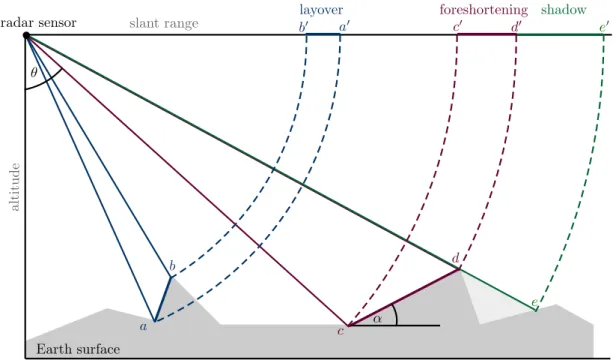
Geometric Properties: Due to the different acquisition principles of optical and SAR satellites (measuring signal travel time vs. angles), the corresponding images further exhibit quite different geometric properties for all objects above the ground. The optical images used in the thesis are acquired through the use of a scanner system. For these kind of systems, above ground objects located perpendicular to the direction of flight get projected away from the sensor in the image plane. The opposite is the case for radar systems, where the image geometry is derived through the traveling time of the backscattered signal. Therefore, above ground objects get projected towards the sensor in the image plane [37]. An illustration of the different image geometries between optical and SAR images is shown in Figure2.4. Here, the different projection (towards and away from the sensor) can be seen for the point clocated on the roof of the house. SAR images further shows three typical distortion effects called foreshortening, layover and shadowing. These effects occur along objects above the ground level and have a strong influence on their visual appearance within the image. Foreshortening denotes the shortening of a distance between two points during the projection in the image plan. This effect occurs if a slope is facing the sensor and has an angleα smaller than the incident angleθ of the SAR sensor or if a slope is facing away from the sensor with an angle smaller than 90◦−θ. Layover appears if a slope is facing the sensor and has an angle higher than the incident angle of the SAR sensor. This effect is particularly common in urban and

Earth surface sensor a′ _b′ c′ d′ a b a′′ b′′ c′′ _d′′ a lt itu d e d b

optical image plane

SAR image plane

b b c b b e b

Figure 2.3: Comparison of optical and SAR imaging. The green (blue) marked lines illustrate the projection of the four pointsatodon the Earth surface into the optical (SAR) image plane. Elevated points such as pointcare shifted away from the sensor in the optical image plane and towards the sensor in the SAR image plane. The pointeis neither seen by the optical nor SAR sensor, and hence not present in the acquired images.

(20)

Earth surface

b

radar sensor layover foreshortening shadow

b a′ b′ a c′ d′ c d e e′ slant range a lt it u de α θ

Figure 2.4: Illustration of the geometric distortion effects layover (marked blue), foreshortening (marked dark red) and shadowing (marked green) for SAR images. Layover: an observed object appears upside down in the image plan; Foreshortening: an observed object or ground segment appears shortened in the image plan; Shadow: non-visible regions appear as dark areas in the image.

mountainous areas. As a consequence, areas affected by overlay appear relatively bright (due to the overlay of the signal response) and buildings and steep mountains can appear upside down in SAR images. Shadowing on the other hand appears, if a terrain slope is oriented away from the sensor and at an angle higher than the incident angles of the sensor. Since no information can be gained from these shadowed regions, these appear as dark areas in the images. Note that all introduced radar effects depend on the viewing direction of the sensor and the geometry of the targeted object on ground. A visualization of the layover, foreshortening and shadowing effect of SAR sensors is provided in Figure 2.4.

Positioning Accuracy: Furthermore, the different acquisition modes have also an effect on the geo-referencing process. The location accuracy of optical satellites depends on a precise knowledge of the satellite orientation in space in order to determine the satellite-viewing direction to ground objects. The required measurements of the attitude angles in space often suffers from insufficient accuracies of the measurements, and are the main reason for a lower geo-localization accuracy of optical satellite data. For example, the absolute geo-localization accuracy of images for optical satellites like PRISM, Worldview-2, or QuickBird ranges from 4 m to 30 m. Images captured by high-resolution SAR satellites on the other hand, exhibit a much higher geo-localization accuracy, mainly due to the availability of precise orbit information and the recent developments in SAR geodesy. More precisely, SAR sensors determine the distance to ground object via the signal traveling time, which can be measured precisely if also atmospheric effects are taken into account, and lead to images with high geo-localization accuracy. The SAR images used in this thesis are acquired by the satellite TerraSAR-X [43] and exhibit an absolute geo-localization accuracy in the range of a few decimeters or centimeters for specific targets [14]. An example of the differences in the

(21)

(a) Digital Orthophoto (GSD=0.2 m) (b) TerraSAR-X image (GSD=0.5 m)

(c) WordView-2 image (GSD=0.5 m) (d) QuickBird image (GSD=0.6 m)

Figure 2.5: Visualization of the absolute geo-localization accuracy of different sensors. The red marked dots and lines represent GPS measurements.

positioning accuracies of optical and SAR satellite images is provided in Figure2.5. The red dots are GPS measurements along the inner circle of the roundabout and represent with an absolute geometric accuracy within a few centimeters the ground truth. Figure 2.5(a) shows a digital orthophoto (DOP), which is accurately geo-referenced and almost perfectly aligned with the GPS measurements. A similar situation can be seen in Figure2.5(b). Here, a TerraSAR-X image of the same scene overlaid with the GPS measurements and the street extracted from the DOP is displayed. Figure 2.5(b) and (d) show the same information but underlaid with a WordView-2 and QuickBird image, respectively. The geo-localization error of both optical images is clearly visible. Furthermore, this error depends on the underlying sensor model and varies between images acquired from different satellites.

Based on the discussed optical and SAR sensor principles and the resulting different image properties, two novel methods for the matching of optical and SAR images will be introduced in Chapter4. In particular, the different radiometric and geometric properties are thereby taken into account in order to enable the exploitation of the high positioning accuracy of SAR data for the positioning improvement of the optical images. In the following Section2.2, the principles of supervised machine learning are presented. The theoretic concepts discussed here form the basis of our later presented optical and SAR image matching methods.

(22)

2.2 Principles of Supervised Machine Learning

In 1959, Arthur Samuel coined the term machine learning and defined it as "a field of study that gives computers the ability to learn without being explicitly programmed" [44]. A more formal definition of machine learning, which mentions the term "learning", was given by Tom Mitshell in 1997: "A computer program is said to learn from experience E with respect to some class of tasks T and performance measure P if its performance at tasks in T, as measured byP, improves with experienceE" [45]. The experienceE is a dataset (a collection of many examples), the task T defines the actually goal of the training, e.g. image denoising or classification, and the performance measure P is usually tailored to the task T with the aim of evaluating the performance of the algorithm, e.g. accuracy measure of a classification problem. The term learning in both definitions refers to the process of attaining the ability to perform a task on the basis of given data or past experience.

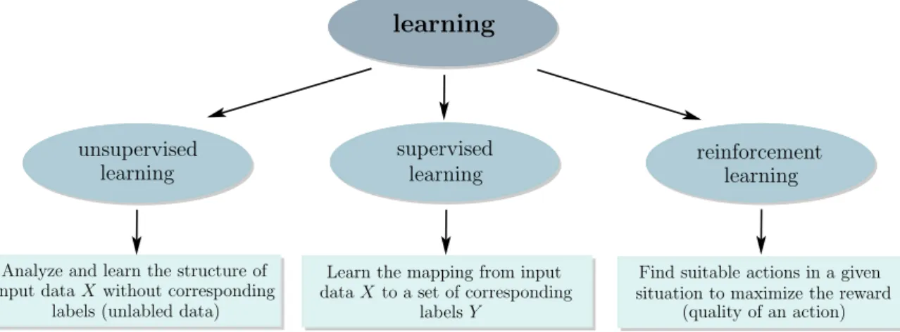
The type of learning depends on the kind of given experience and broadly divides machine learning algorithms into three categories. The first class, supervised learning, tries to learn the mapping from input data X to a set of corresponding labels Y (labeled data) and is commonly applied on regression or classification problems. The second class, unsupervised learning, deals in contrast with the problem of analyzing and learning the structure of the input dataX without corresponding labels (unlabeled data), e.g. clustering or density estimation. The last class, reinforcement learning, handles the problem of finding suitable actions in a given situation to maximize a reward. The reward is defined by the quality of the action and the learning is realized through a trial and error process (the algorithm is not provided with the optimal actions). The diagram in Figure 2.6 comprises an overview and the general ideas of the three learning types.

The structure of any machine learning algorithm has to be carefully designed before the learning step in order to fulfill the needs and requirements of a particular task. The key of each machine learning algorithm are trainable parameters, often called weights, which are optimized during the learning process. Applying a machine learning algorithm to solve a specific task, commonly involves the following three phases: (1) the learning or training

learning reinforcement supervised learning

learning

learning unsupervised labelsY

Find suitable actions in a given situation to maximize the reward Learn the mapping from input

Analyze and learn the structure of input dataX without corresponding

labels (unlabled data) dataX to a set of corresponding (quality of an action)

Figure 2.6: Overview and general idea of the three types of learning: unsupervised, supervised and reinforcement learning.

(23)

phase, (2) the validation phase and (3) the test or inference phase. In the following, we will discuss the aim and process of these phases in the context of supervised learning. More information about unsupervised learning can be found in [46–48] and about reinforcement learning in [47,49].

Supervised Learning - the General Goal

The goal of a supervised learning algorithm is to learn a function

f :X→Y , (2.1)

when a set of input data X and a set of corresponding labels Y are given. The function

f assigns every inputx∈X to an output y∈Y given a set of labeled input-output pairs D=nx(n),y(n)|n= 1, . . . , N and N ∈_No. The variablesxandy can be scalars, vectors or matrices. If the elements of yare continuous, it is called a regression problem, and if the elements are discrete, it is called a classification problems. The functionf is often referred to as the model and is defined by the set of trainable parameters θ. The assigned values y=f(x,θ) are commonly called the predictions of the model. Before starting the actual learning process, the set of given input output pairs Dis partitioned into three subsets, a training D_train, validation D_val and test setD_test.

Training Phase: The aim of the training phase is to find the optimal parametersθ based on the given training data. In order to find an optimal approximationf(θb) of the true but unknown functionf∗ (given D_train) the quality of the model has to be evaluated. In the case of supervised learning the quality of a model can be measured by regarding the error in the model predictionsy_b(n)=f(x(n),θb). This measure is often called the loss, error or cost function and is defined as

L(y(n),yb (n)_{) =}    0 ify_b(n) =y(n) >0 otherwise . (2.2)

The loss function enables to penalize incorrect model predictions (y_b(n) 6=y(n)) during the training process. The optimal model parametersθ∗ are computed by minimizing the overall error, which gradually increases the quality of the learned model

θ∗ = arg min θ N X n=1 L(y(n),yb (n)₎_. _(2.3)

This procedure will lead to a model, which is able to provide accurate predictions for input values from the training set, but not necessary for unseen data. In order to find a model which further provides accurate predictions for unseen data and, hence, is applicable to a real world task, the networks ability to generalize has to be monitored during the training.

Validation Phase: The validation phase pursues the goal of estimating the generalization performance of the trained model. Therefore, the performance of the model is measured by evaluating the loss functionL on the validation dataset. The training and validation phase can be executed alternately till the best model is found. Commonly, the model showing the best performance on the validation set is picked as the best and final model. A second purpose

(24)

16 2. Theoretical Background unsupervised learning

learning

learning supervised _{reinforcement} learning discriminant function model discriminative generative model

which maps input learns directly a function,

the conditional probability the joint probability dataxto labelsyk _{distributions}_p₍_y

k|x) distributionsp(x, yk) learn the mapping from input

xto labelsykby estimating xto labelsykby estimating learn the mapping from input

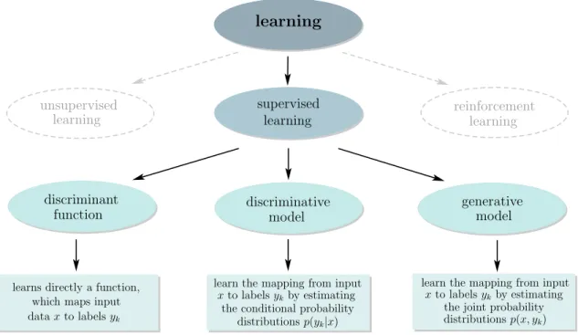
Figure 2.7: Overview and general idea of the three branches of supervised learning: discriminant functions, discriminative models and generative models.

of the validation phase is to tune the hyperparameters of the model. Hyperparameters are model configurations, which are set before the actual learning is realized and cannot be directly learned during the training phase. In order to tune them, algorithms like grid search or random search are often used.

Test Phase: The aim of the last phase, called test phase, is to evaluate the performance of the final model on an independent test dataset. As in the training and validation phase, the performance is measured by utilizing the loss function L. Since the test set contains only unseen data (not used for the training or validation phase), this step reveals the ability of the model to generalize to unseen data and its quality to perform on the desired task. The quality of the final model depends next to the chosen type and complexity of the algorithm, the set of hyperparameters, the loss function and the optimization procedure also on the quality and amount of the given training data. It is important that the selection of the set of data pairs (X, Y) represents the real task and that the distribution of the data is a good approximation of the real data distribution. Furthermore, the right balance between the complexity of the model and the amount of training data with respect to the actual task has to be found to limit the generalization error. In this context terms like under- or overfitting a commonly used, which will be thematized in Subsection 2.2.1.

Supervised Learning - the Types of Learning

Supervised learning algorithms can be further divided into three subcategories depending on how the mapping from X to Y is actually learned during the training phases (shown in Figure 2.7). The first category comprises discriminant functions, which define a class of algorithms that try to find directly a function which maps an input value x to an output label y (non-probabilistic algorithms). The learned model does not provide any confidence

(25)

or a probability for an output labely. If we consider a simple classification problem (such as illustrated in Figure 2.8), where X is a set of images (represented as colored dotes) and Y a set of kinds of animals shown in the image (cat, dog or elephant), a discriminant function will try to learn the decision boundaries between the classes, which divide the feature space into separate areas. Depending on the learned decision boundaries, new images would be assigned to a label without providing the uncertainty of the model.

Figure 2.8: Illustration of a simple classification problem with three classes (red, yellow and green dots) and the corresponding decision boundaries (black lines). The gray line marks a possible non-optimal decision boundary during the training phase of the discriminant function.

The second class are discriminative models, which define a class of algorithms that try to learn a statistical model to estimate the conditional (posterior) probability distributions

p(y|x) from input datax∈X to labels y∈Y (probabilistic algorithms). The distributions

p(y|x) provide the probabilities of each label y given a fixed input value x. The goal of assigning or predicting a label to each input value xis realized by evaluating the function

f(x) = arg max

y∈Y p(y|x). (2.4)

Discriminative models learnp(y|x) directly from the data and do not consider the underlying data distribution. In contrast to discriminant functions, discriminative models provide next to the predicted label for a given input data also the corresponding conditional probabilities. This additional information helps to evaluate the confidence of the model regarding a certain prediction.

The last class, generative models try to learn the joint probability distributions p(x, yk), or

in other words, they try to explicitly model the distribution behind the data. In the case of generative models the predicted label of an input valuexis determined by evaluating the function

f(x) = arg max

y∈Y p(x,y). (2.5)

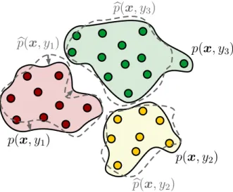
The example in Figure2.9 shows the same classification example as in Figure2.8, but this time handled via a generative model. A generative model tries to learn the joint probability distributions p(x, y1), p(x, y2) and p(x, y3) of input data x and the tree classes labels y1, y2 andy3. The red green and yellow area in Figure2.9mark the areas in the image space,

(26)

which contain (with a high probability) real images showing cats, dogs or elephants. The goal of the training procedure is to minimize the distance to the true data distribution. To measure the distance to the true data distribution a measure such as the Kullback–Leibler divergence can be applied.

The choice of the optimal learning type heavily depends on the actual problem. Generative models are more expensive to compute and learning p(x,y) is generally more difficult than learningp(y|x) or directly learning the mapping fromXtoY. On the other hand, generative models perform in principle better when larger training sets are given and are richer in the sense that they implicitly model p(y|x) andp(x) throughp(x,y), which is given through the following equation

p(x,y) =p(x)·p(y|x) (Bayes’ Theorem). (2.6) Generative models further provide the possibility of sample new data pairs (x,y) from

p(x,y). If we consider the animal image classification example with the three possible classes (cat, dog or elephant) a generative model is able not only to predict a label for a new input image, but also to produce synthetic images (data points) belonging to one of the three classes. However, discriminative models are mostly more robust w.r.t. modeling errors and blunders and regarding a classification problem, where only a decision boundary is needed to separate the classes, a discriminant function or a discriminative model generally perform better.

In the following two subsections, we will introduce the concepts and provide insights of a discriminative model, neural networks, and a generative model, generative adversarial networks (GANs). For more information about discriminant functions and discriminative and generative models we refer to [46,47] and for a detailed discussion about discriminative and generative classifiers to [50].

bm

p

(

x

, y

1

)

b

p

(

x

, y

1

)

b

p

(

x

, y

3

)

b

p

(

x

, y

2

)

p

(

x

, y

3

)

p

(

x

, y

2

)

Figure 2.9: Illustration of a simple classification problem with three classes (red, yellow and green dots) and the corresponding joint probability distributionsp(x, y1),p(x, y2) andp(x, y3). The gray dashed lines illustrate possible (non-optimal) joint probability distributions p_b(x, y1), p_b(x, y2) and

b

(27)

2.2.1 Artificial Neural Networks

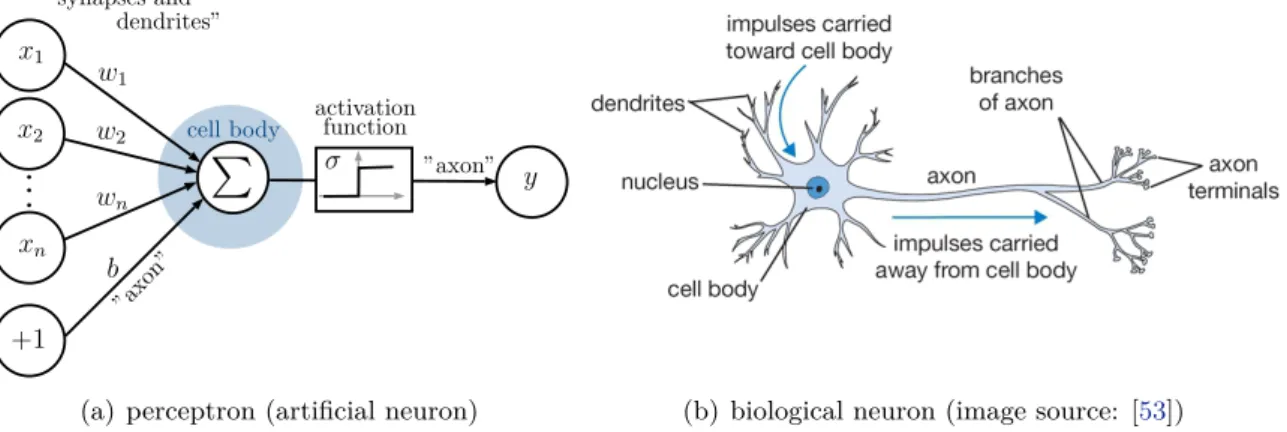
The origin of artificial neural networks (ANNs) dates back to the early 1940s where McCulloch and Pitts [51] developed the first concepts of the functional principles of biological learning system such as the brain. Inspired by this work, Rosenblatt developed the concept of perceptrons [52] in the late 1950s. A perceptron, often called artificial neuron, is a model of a biological neuron and can be understood as a computational unit which produces a single output y given some inputx. The outputy is given through the following equation

y=σ n X i=1 wixi+b ! =σwTx+b, (2.7)

where the values xi (i = 1, . . . , n) are the input elements, wi the learnable weights, b

the learnable bias andσ(·) the activation or transfer function. The weights represent the importance of the corresponding input value and are adjusted during the training phase. The activation functions serves as a threshold, which divides the input space into two partitions. Commonly, non-linear activation functions are applied in order to introduce non-linearities into the perceptron and later to the network (otherwise only linear functions can be modeled). The optimal bias is learned during training and enables a shift of the activation function in the image space in order to find the optimal partition of the input data. An illustration of a perceptron and the comparison with the biological neuron counterpart is shown in Figure 2.10.

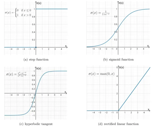
In the original work [52], Rosenblatt proposed the application of a step function as activation function, whereas nowadays non-linear functions such as the sigmoid, the hyperbolic tangent or rectified linear functions are usually applied (see Figure 2.11). This development can be traced back to an unstable behavior caused by a step function: small changes in the input values can lead to huge changes in the output value, which complicates a gradually adjustment of the weights, and hence complicates the training procedure.

A single perceptron is only capable of learning a linear separation of the input data, heavily limiting the number of application cases. This drawback can be overcome by composing

b b b

P

y +1 x2 xn x1 w1 wn w2 b cell body σ ”axon” ”synapses and dendrites” ”axo n” activation function

(a) perceptron (artificial neuron) (b) biological neuron (image source: [53]) Figure 2.10:Illustration and comparison of a: (a) perceptron (artificial neuron) and (b) biological neuron model. The values (x1, . . . , xn) are the input values, (w1, . . . , wn) the corresponding weights andbthe bias of the perceptron.

(28)

σ(x) =

(

0 ifx_≤0 1 ifx >0

(a) step function

σ(x) =₁₊1_e−x (b) sigmoid function σ(x) =ex−e−x ex+e−x (c) hyperbolic tangent σ(x) = max(0, x)

(d) rectified linear function

Figure 2.11: Example of four non-linear activation functions: (a) a step function, (b) the sigmoid function, (c) the hyperbolic tangent and (d) a rectified linear function.

several perceptrons (artificial neurons) and connecting them to a directed acyclic graphi, called an artificial neural network or sometimes a multi-layer perceptron (MLP). Figure 2.12 shows a simple representation of a neural network. The nodes of the graph are usually called units and represent artificial neurons. Commonly, a neural network is built of distinct layers, where the first layer is called the input layer and the last one the output layer. All layers in between are called hidden layers. In the shown example the neurons within one layer share no connections but between two adjacent layers the neurons are fully pairwise connected. Such a layer structure is called fully-connected. If the information is only fed forward through the network (only the output from previous layers is fed as input to the later layer), it is called a feedforward neural network.

The network architecture can vary in the number of input, hidden and output units, the number of hidden layers and the type of layers (overview of different layer types follows below). A network with only one hidden layer is called a shallow neural network and with more than two layers a deep neural network. The task of the layers is to extract information (features) from the input data. The complexity of the features extracted by the layers increases along with the depth, where early layers commonly detect simpler features, such as edges or corners, and later layers more complex features, such as parts of a human face.

i

(29)

2. Theoretical Background 21 +1 x2 x3 x1 +1 y1 y2 +1 hidden layers output layer input layer W(1₎ W(2₎ W(3₎ b(1₎ b( 2₎ b( 3₎ l₁ l₂ l₃ l₄

Figure 2.12: Example of an artificial neural network with four layers (the input layerl1, two hidden layers l2 and l3 and the output layer l4), which maps the input x = (x1, x2, x3) to the output y= (y1, y2). Each circle represents a unit in the network and the arrows the connections between the units of adjacent layers. The unit marked with +1 represents the bias unit of the corresponding layer. The matrix W(t)contains the weights between layertandt+ 1 and the vectorb(t)the biases from layertto t+ 1.

Neural Networks - The Training Process

In order to train the network to learn meaningful features for solving a specific task, a loss function has to be defined. Since we are still assuming a supervised learning problem, the initial situation is the same as described in Subsection 2.2. The goal is to learn a model that predicts an output y_b given and input x on the basis of a training dataset Dtrain =

n

x(n),y(n)|n= 1, . . . , N and N ∈_No. Utilizing the mean square error (MSE) to measure the error in the predictions, the loss function for one training example can be expressed as Ly(n), fW,b x(n)= 1 2 fW,b x(n)−y(n) 2 , (2.8)

where W is a matrix containing all weights and b a vector containing the biases of the network. The overall set of learnable parameters is given by θ= (W,b). The predictions

b

y(n)=fW,b

x(n)are obtain by computing a forward pass through the network (forward propagation) and can be computed by evaluating a chain of function (vectorized notation)

fW,b

x(n)=a(L) with a(t+1) =σh(t+1)

h(t+1) =W(t)a(t)+b(t) (t= 1, . . . , L−1).

(2.9)

Here,Ldenotes the total number of layers, a(t)_{is a vector containing the so called activation}

valuesa(_it) of unit iin layer twith a(1)=x(n), h(t) is a vector containing the valuesh(_it) of uniti in layer t(hidden values),W(t) is a matrix containing all the weights w_i,j(t) between unitiin layert and unitj in layert+ 1, and b(t) is a vector containing the biasesb(_it) from layert to unit iin layer t+ 1. A visual example of the terms is illustrated in Figure2.13

(30)

and the detailed expression of h(t+1) is given by the following equation

h(t+1) =        w(₁t_,)₁ w₁(t_,)₂ · · · w(₁t_,n)_t w(₂t_,)₁ w₂(t_,)₂ · · · w(₂t_,n)_t .. . ... . .. ... w_n(t_t)₊₁_,₁ w_n(t_t)₊₁_,₂ . . . wn(tt)+1,nt        | {z } W(t) ·        a(₁t) a(₂t) .. . a(ntt)+1        | {z } a(t) +        b(₁t) b(₂t) .. . b(ntt)+1        | {z } b(t) , (2.10)

wherent is the number of units in layert. The overall error E(W,b) is given by the sum

overall training examples in D_train. The goal of the training phase is to find the optimal set of parameters θ= (W,b), which minimize the overall error. This optimization problem can be stated as follows c W,bb = arg min W,b N X n=1 Ly(n), fW,b x(n) | {z } =E(W,b) . (2.11)

Before applying an optimization algorithm the parameters θ of the network have to be initialized. The weights are commonly initialized by small random values, or a specific initialization scheme such as proposed in [54], or with weights from a pre-trained network and the biases set to zero. If all weights would be initialized with the same value, every activation a(_it) would be the same and, hence, every neuron would learn the same. For a detailed overview of parameter initialization strategies and its advantages and disadvantages we refer to [48] and for the specific ones used in this thesis to Subsections 5.3.1and 5.2.1.

h(2) 2 →a (2) 2 w₂(2) ,1 l₂ l₃ w(2) 2,3 h(3)₂ →a(3)₂ h(2)₁ →a(2)₁ h(2)₃ →a(2)₃ +1 b(2) 2 w(2)₂ ,2

Figure 2.13: Illustration of the forward propagation for one unit in a neural network and the computation of the term h(3)₂ and the activation value a(3)₂ of the second unit in layer 3. The values a(2)_i are the activations of the i-th unit in layer 2,w(2)₂_,j are the weights between thej-th unit in layer 2 and the second unit in layer 3 andb(2)₂ the bias from layer 2 to the second unit in layer 3.

(31)

error

traning time learning rate too small

learning rate too high

optimal learning rate

Figure 2.14:Influence of the learning rate on the error over the training time.

After the initialization of the parameters, an optimization algorithm such as gradient descent is applied to minimize the overall loss w.r.t. to the parameters. The idea of gradient descent is to learn the optimal parameters by updating the weights and biases in an iterative way

w_i,j(t) ←w_i,j(t)−λ∂E(W,b) ∂w(_i,jt)

b_i(t) ←b_i(t)−λ∂E(W,b) ∂b(_it) ,

(2.12)

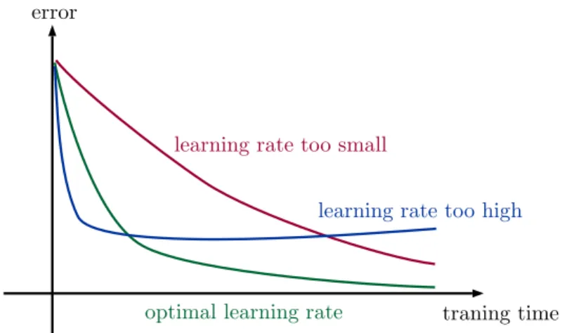
where the parameter λis called learning rate and determines the speed of the parameter updates. The learning rate has often a significant influence on the success of the learning and represents a hyperparameter, which has to be determined before the learning phase and tuned by utilizing the validation phase. Figure2.14exemplifies the influence of the learning rate on the overall error during training. A too small learning rate lead to a slow convergence of the loss function, whereas a too high learning rate can lead the loss to oscillate around the minimum or to diverge.

So, far the total error E(W,b) is computed by summing up the loss function over the whole training set D_train in one iteration of gradient descent. A common approach for the training of a neural networks is to evaluate the error only over a small subset of Dtrain,

called (mini-)batch. The batches can be chosen randomly from Dtrain in each iteration

or generated beforehand by partition the setD_train into several batches. An advantage of this strategy is that it is computationally faster (in the case of a larger training set Dtrain).

Furthermore, it converges faster, while providing a reasonable approximation of the total error due to redundant information in most datasets. This extension of gradient descent is called (mini-batch) stochastic gradient descent (SGD), where the key step of SGD is to compute the partial derivatives ∂E(W,b)

∂w(_i,jt) and

∂E(W,b)

∂b(_it) .

In 1986, Rumelhart et al. [55] proposed an algorithm for the computation of these derivatives, which enabled the efficient training of neural networks. The algorithm is called back-propagation and is based on the idea of propagating the error backwards through the network

(32)

by applying the chain rule

∂f(g(x)) ∂x = ∂f(g(x)) ∂g(x) · ∂g(x) ∂x . (2.13)

We will introduce the idea of back-propagation in the following and simplify the notations without loss of generality by exploiting the following rule

∂E(W,b) ∂w_i,j(t) = ∂ Nb P n=1 LW,b,x(n),y(n) ∂w(_i,jt) = Nb X n=1 ∂LW,b,x(n),y(n) ∂w_i,j(t) (2.14)

and consider only the error caused by one training examplex(n)_,_y(n)_{and the corresponding}

derivatives ∂L(W,b) ∂w(_i,jt) := ∂L(W,b,x(n)_,_y(n)₎ ∂w(_i,jt) and ∂L(W,b) ∂b(_it) := ∂L(W,b,x(n)_,_y(n)₎

∂b(_it) . In the above stated

equation the term Nb denotes the size of the batch.

The output of the network is computed through the forward propagation and is defined by a chain of functions (see Equation 2.9). Therefore, the chain rule can be applied and the derivative of L(W,b) with respect to a single weightw(_i,jt) between unit iin layertand unit

j in layert+ 1 can be rewritten as

∂L(W,b) ∂w_i,j(t) = ∂L(W,b) ∂h(_it+1) ∂h(_it+1) ∂w(_i,jt) = ∂L(W,b) ∂a(_it+1) ∂a(_it+1) ∂h(_it+1) ∂h(_it+1) ∂w(_i,jt) = nt+2 X k=1 ∂L(W,b) ∂h(_kt+2) ∂h(_kt+2) ∂a(_it+1) ! ∂a(_it+1) ∂h(_it+1) ∂h(_it+1) ∂w(_i,jt) = nt+2 X k=1 ∂L(W,b) ∂h(_kt+2) w (t+1) k,i ! σ0h(_it+1) | {z } ∂L(W,b) ∂h(t+1) i a(_jt), (2.15)

wherent+2 denotes the number of units in layert+2. For an efficient computation of the

derivatives the error term δ_i(t) is introduced and recursively defined for t = 1, ..., L−1 as follows δ(_it):= ∂L(W,b) ∂h(_it) = nt+1 X k=1 δ_k(t+1)w_k,i(t+1) ! σ0h(_it), (2.16)

where the first values ofδ(_iL) (error term of the output layer) are given by

δ_i(L)= ∂L(W,b) ∂h(_iL) = ∂L(W,b) ∂a(_iL) ∂a(_iL) ∂h(_iL) = ∂L(W,b) ∂a(_iL) | {z } (_by(n)₋_y(n)₎ σ0h(_iL). (2.17)

The error termδ(_it) measures the error of each neuron iin layertand starting from δ_i(L) the error can be propagate backwards through the network (backpropagation). An illustration of the computation of the error term for a single neuron is illustrated in Figure 2.15.