Wayne State University Theses
1-1-2015
Survival Analysis Approach For Early Prediction Of
Student Dropout
Sattar Ameri
Wayne State University,
Follow this and additional works at:https://digitalcommons.wayne.edu/oa_theses
Part of theComputer Sciences Commons
This Open Access Thesis is brought to you for free and open access by DigitalCommons@WayneState. It has been accepted for inclusion in Wayne State University Theses by an authorized administrator of DigitalCommons@WayneState.
Recommended Citation
Ameri, Sattar, "Survival Analysis Approach For Early Prediction Of Student Dropout" (2015).Wayne State University Theses. 443.
STUDENT DROPOUT
by
SATTAR AMERI THESIS
Submitted to the Graduate School of Wayne State University,
Detroit, Michigan
in partial fulfillment of the requirements for the degree of
MASTER OF SCIENCE
2015
MAJOR: COMPUTER SCIENCE Approved by:
SATTAR AMERI 2015
To my dear wife for her devoted support.
DEDICATION . . . i LIST OF TABLES . . . iv LIST OF FIGURES . . . v CHAPTER 1 INTRODUCTION . . . 1 1.1 Overview . . . 1 1.2 Motivation . . . 2 1.3 Problem Statement . . . 5 1.4 Thesis Contributions . . . 6
1.5 Organization of the Thesis . . . 7
CHAPTER 2 STUDENT DROPOUT PREDICTION . . . 8
2.1 Literature Review . . . 8
2.2 Prediction Models . . . 10
2.2.1 Regression . . . 10
2.2.2 Logistic Regression . . . 11
2.2.3 Support Vector Machines (SVM) . . . 11
2.2.4 Adaptive Boosting . . . 12
2.2.5 Decision Tree . . . 13
CHAPTER 3 PROPOSED SURVIVAL ANALYSIS APPROACH . . . 15
3.1 Survival Analysis . . . 16
3.1.1 Survival and Hazard Functions . . . 17
3.1.2 Censored Data . . . 19
3.1.3 Maximum Likelihood Function . . . 20
3.1.4 Non-parametric and Parametric Survival Models . . . 21
3.2 Cox Proportional Hazard Model . . . 22
3.2.1 Parameter Estimation . . . 23 ii
CHAPTER 4 EXPERIMENTAL RESULTS . . . 30
4.1 Data Description . . . 30
4.2 Preliminary Analysis of the Data . . . 32
4.3 Evaluation Metrics . . . 37
4.4 Performance of Various Classification Methods . . . 39
4.5 Evaluation on Predicting Semester of Dropout . . . 41
CHAPTER 5 CONCLUSION AND FUTURE WORK . . . 50
REFERENCES . . . 52
ABSTRACT . . . 57
AUTOBIOGRAPHICAL STATEMENT . . . 58
3.1 Notations used in this thesis. . . 17
3.2 Example of survival data . . . 27
3.3 Example of survival data after counting process reformatting . . . 27
4.1 Description of attributes used to build our dataset. . . 33
4.2 Coefficient estimation of the attributes from the Coxph model . . . 40
4.3 Performance of Logistic regression, Adaboost and Decision tree with Coxph and TD-Cox on WSU student retention data from 2002 to 2008 (experiment 1) for each semester using 10-fold cross validation along with standard deviation. . . 42
4.4 Performance of Logistic regression, Adaboost and Decision tree with Coxph and TD-Cox on 2009 WSU student retention (experiment 1) for each semester along with standard deviation. . . 43
4.5 Performance of Logistic regression, Adaboost and Decision tree with Coxph and TD-Cox on WSU student retention data from 2002 to 2008 (experiment 2) for each semester using 10-fold cross validation along with standard deviation. . . 44
4.6 Performance of Logistic regression, Adaboost and Decision tree with Coxph and TD-Cox on 2009 WSU student retention (experiment 2) for each semester along with standard deviation. . . 45
4.7 Performance of linear regression, SVR and Cox methods in predicting the semester of dropout on WSU student retention data (experiment 1) from 2002 to 2008 for each semester using 10-fold cross validation and 2009 student retention data. . . 48
4.8 Performance of linear regression, SVR and Cox methods in predicting the semester of dropout on WSU student retention data (experiment 2) from 2002 to 2008 for each semester using 10-fold cross validation and 2009 student retention data. . . 48
1.1 Process flowchart of graduation for a college student. . . 3 3.1 Illustration of the student retention data using survival concepts. . . . 20 3.2 Flowchart of proposed survival analysis framework for student
reten-tion problem . . . 29 4.1 An illustration to demonstrate second experiment. . . 32 4.2 Histogram plot for the percentage of dropout per semester . . . 34 4.3 Histogram plot for some of the important pre-school attributes: (a)
Gender, (b) Ethnicity, (c) High school GPA, (d) ACT composite score, (e) College and (f) Year of admission . . . 35 4.4 Probability of attrition for 4 different variables: (a) gender, (b) county
of residency, (c) ethnicity and (d) high school GPA. It should be noted that all other variables fix on an average for each case. . . 36 4.5 Performance of different methods obtained at different semesters
(ex-periment 1): (a), (c) and (e) are the results of 10-fold cross validation on 2002-2008 training data and (b), (d) and (f) are the results for 2009 test dataset. . . 46 4.6 Performance of different methods obtained at different semesters
(ex-periment 2): (a), (c) and (e) are the results of 10-fold cross validation on 2002-2008 training data and (b), (d) and (f) are the results for 2009 test dataset. . . 47
CHAPTER 1
INTRODUCTION
1.1
Overview
One of the long-term goals of any university in the U.S. and around the world is in-creasing the student retention. The negative impacts of student dropout are clear to stu-dents, parents, universities and society. The positive effect of decreasing student attrition is also self-evident including higher chance of having a better career and higher standard of life for college graduates. Not only from student perspective but also college rankings, federal funding agencies and state appropriation committees are all directly dependent on by student retention rates. Thus, the higher the student retention rate, the more likely that the university is positioned higher in the ranking, secure more government funds, and have easier path to program accreditations. In view of these reasons, direc-tors in higher education feel increasingly pressurized to outline and implement strategies to increase student retention.
In this thesis, firstly, we provide a detailed analysis of the student attrition problem and predict the risk of dropout at Wayne State University. Methods that are currently being used for the problem of student dropout are the standard preliminary statistical approaches. Our work has a number of advantages with the potential of being employed by higher education administrators at various universities. We take advantage of multiple kinds of information about different aspects of student’s characteristic and efficiently utilize them to make a personalized decision about the risk of dropout for a particular student.
In the second part of this thesis, we propose survival analysis model for the student retention problem. Survival analysis method has been shown to be successful in other applications such as healthcare and biostatistics. Although well suited as a statistical
technique to study student dropout, survival analysis has not been used efficiently in this study domain. With survival analysis, we also address the challenge of “time to event occurrence”. This is critical in the student retention problems because not only correctly classifying whether student is going to dropout or not is important but also when this is going to happen is crucial to investigate for further interventions. In such cases, the reliable estimation of risk at early stage of student education is very important. We propose a novel framework that uses both pre-enrollment and semester-wise information to address this issue. The basic idea here is to utilize the survival analysis method at early stage of college study to predict student success.
1.2
Motivation
The problem of college student retention is very important for educational researchers, managers, and the higher education members. Costs accrue to society, the institution, and the student when the student degree completion is not realized [30]. From a so-cietal perspective, the achievement of a college diploma improves mediate background resources, like family economic situation. Thus, it impacts the subsequent occupational status, potential earnings, and social status achievement [37]. This fact is proved by the difference between social situation achievements of every single person from the same level of economic condition with different levels of educational degree [30]. From the in-stitution’s perspective, maintaining enrollments is important for the economic stability. As the number of new students have fluctuated, finding the characteristics of students that remain enrolled and graduate is very important. Figure 1.1 demonstrates a process flowchart of graduation for a college student. Universities and colleges and all other institutions become fully aware of this fact that the primary assets needed to recruit, enroll, enlist, register, advise and assist a new student are the same whether that student remains and graduates or not. For instance, publication and marketing expenses, costs associated with maintaining a staff of professional counselors, travel costs connected with
conducting college fairs and informational meetings, costs related with tele-counseling, staff time contacting students for yield enhancement, and staff time conducting academic advising, are all examples of pre-enrollment expenses experienced by the institution. Al-together, finding a better understanding of which college students are more likely to register and remain enrolled, is significant for maximizing those pre-enrollment resources and generating revenue.
Figure 1.1: Process flowchart of graduation for a college student.
Understanding student graduation behaviours can influence the improvement or en-hancement of retention strategies and prompting a higher graduation rate. In addition, graduation rates are progressively employed as a measure of a college’s efficiency and are sometimes linked to resource allocation. Graduation data is needed as a component of the “Common Data Set”, a reliable set of information given by individual institutions as a way for future college students and their families to make reasonable comparison among other institutions. Graduation information is also needed by other media, like “World Report” or “US News” to give rating to institutions and provide an extra asset for comparison. Thirty states including Michigan have a funding formula that allocates some amount of funding according to efficiency indicators like time to degree, transfer rates, the number of minority and low-income graduates, the number of degrees awarded
and course completion. More precisely this formula considers 6 parameters for total score for funding:
1- Undergraduate degree completions in critical skill areas 2- Research and development expenditures
3- Six-year graduation rate 4- Total degree completions
5- Institutional support expenditures as a percentage of total core expenditures
6- Pell Grant students where in Fiscal year 2014-15 in Michigan 37.3 million dollars for universities and 8.9 million dollar for community colleges were allocated based on the above performance metrics. 1
In higher education we define student retention rate as the percentage of students who after completing a semester, return to the same university for the following semester. Stu-dent retention rate not only has effect on the university but also can affect the nearby cites. An institution’s retention rate influences the job opportunities for students and public opinion. Universities are eager to find out which factors or attributes are impor-tant for their students’ retention, how they can address this issue and with help of this kind of analysis they can improve their retention rate. It is important because higher re-tention rate will increase university funding from state and also help them to recruit more students and faculty in order to give better service to the community. College student graduation rates are often used as a measure of institution’s performance. However, on the other hand, the dropout rate can show university failure to persuade student success-fully finish their school. These kinds of analyses play a significant role for universities’ decision about how to expand their majors’ capacities and how to allocate financial aid between students. It is not beneficial to give financial aid to who are at high risk of drop out. More important is that the universities are accountable for attrition rate in their
colleges and hence they will be penalized with narrowing their funds. In recent years, the cost of higher education has increased continuously and the amount of fund from state and federal governments that colleges received is decreased and hence the universities should try to spend their funds very wisely and doing this without analytical studies is not feasible.
From the university point of view, maintaining enrollment is important for economic stability, institutional success and managing resource allocation. From the students’ perspective, it will result in higher chance of graduation that leads to higher chance of getting a good job, earn more money and a better life style in the future. In general, knowing the reasons for student dropout can help the faculty and administrators to take necessary actions so that the success percentage can be improved.
1.3
Problem Statement
First-year students have significantly increased during recent years and consequently it resulted in a huge volume of educational data. Thousands of students are admitted to study at universities every year but after first year of study some of them dropout from school. Thus, monitoring and supporting them is a topic that needs consideration at many educational institutions. University staff would like to encourage such students to finish their studies but it is hard to identify them at their early stages. It is important to explore effective approaches for predicting student dropout as well as identifying the factors affecting it with a sufficiently high accuracy. As an example at the College of Engineering of Wayne State University, for the academic year 2012, the dropout rate of freshmen is about 25% in the first year and it increases to 35% after passing two years of study which shows the importance of modeling student dropout early during their study. This thesis is intended to not only find out whether a student drop out or not but also aims at estimating the semester of dropout using survival analysis model.
the most common measure in the academic research domain is retention rate. Students may stay in school and graduate or they do not. Thus, retention models usually predict a binary dependent variable, whether students dropout (coded as “1”) or do not dropout (coded as “0”). Analysts then typically build models using any predictive methods that are appropriate when the dependent variable is binary. Thus, in this thesis we try to answer two questions; first, which students are going to dropout? (using both pre-enrollment information and semester-wise data) and second, when the student is going to dropout? For the first question we develop survival analysis method: Cox and TD-Cox (time dependent Cox) and compare the result with other classification methods such as decision tree, adaptive boosting, and logistic regression and for the second question, we develop Cox model and compare the result with linear regression and support vector regression where censored data are not considered. However, one question that arises is “Why previous classification and regression methods are not appropriate to use for the student retention problem”. Basically, as mentioned earlier, survival analysis methods were shown to be successful in other applications such as healthcare and biostatistics but has been used very infrequently for this research problem. In the presence of censored data, the traditional methods such as linear regression or logistic regression typically fail because these methods cannot consider observations with censored data. Hence, in this work, a novel framework is proposed to use both pre-enrollment and semester-wise information to address the student dropout problem issue.
1.4
Thesis Contributions
To find an answer for the student retention problem discussed above, we introduce an intuitive survival analysis technique. Thus, the main contributions of this thesis are summarized as follows:
• Rigorously define the student attrition problem and create important variables that influence the student dropout.
• Propose a novel early student retention framework which can deal with both ques-tions: “who is going to dropout” and “when the dropout occurs”.
• Using survival analysis methodology to study the temporal nature of student re-tention by incorporating semester-wise student information into the model and focusing on dropout information as the outcome of interest.
• Demonstrate the performance of the proposed method using Wayne State Univer-sity student enrollment data and compare with the existing state-of-the-art meth-ods.
1.5
Organization of the Thesis
The rest of the thesis is organized as follows. In chapter 2 we define student dropout problem and explain the important variables along with some standard prediction meth-ods. In chapter 3, we propose a student dropout prediction model based on survival analysis methods. Chapter 4 demonstrates the experimental results and shows the prac-tical significance of our work using Wayne State University student data. Finally, chapter 5 concludes our discussion along with some future research directions in this area.
CHAPTER 2
STUDENT DROPOUT PREDICTION
In higher education, student dropout rate can be defined as the percentage of students who, after completing a semester, do not return to the same university for the following semester. Universities are eager to find out which factors or attributes are important for the students’ retention. It is important because higher retention rate will increase university funding and also help them to recruit more students and faculties in order to give a better service to the community. College student graduation rates are often used as a measure of institution’s performance. These kinds of analyses play a significant role for universities’ decision about how to expand their majors’ capacities and how to allocate financial aid between students.
2.1
Literature Review
Event prediction is an important area of research where the goal is to predict the occurrence of an event in the data [18]. In higher education, many modeling techniques were found to help educational institutions to predict at-risk students [28]. This results in planning for interventions and better understanding and addressing fundamental issues that cause the student attrition problem. In the past decades, comprehensive models have been developed to address the college student attrition problem. Most of the earlier studies try to understand the reasons behind student dropout by developing theoretical models [38]. For many years, statistical methods have been used widely to predict student dropout and also find the important factors that have some effect on this prediction [22, 43]. Regression is one of the primary techniques that has been applied in this area [11]. Logistic regression is another statistical method that was frequently used in this domain [8, 24]. [25] used logistic regression, discriminant analysis and regression tree to address this issue. In another work, logistic regression method is developed to identify
freshman at risk of attrition within few weeks after freshman orientation [15].
Recently, many researchers in the area of machine learning and data mining tried to address the student retention phenomenon in college and university [10, 35, 41]. Genetic algorithms for selecting feature subset and artificial neural networks for performance modeling have been developed to give better prediction of first year high risk students to dropout at Virginia Commonwealth University [1]. Several classification algorithms including Bayes classifier [3, 29], Decision tree [17, 32, 42], Boosting methods and support vector machines [44] have been developed to predict student attrition rate with higher accuracy compared to the traditional statistical methods.
A slightly more complex and relevant modeling technique is survival analysis. Survival analysis is a subfield of statistics which aims at modeling longitudinal data where the outcome variable is the time until an occurrence of event [23, 26]. In this type of regression model, both components, (i) if an event (i.e. dropout) occurs or not and (ii) when the event occurs can be incorporated simultaneously [27]. So we can assign the probability of dropout for a single period of time and we can also assign a probability for each time period (e.g., semesters) [9]. Thus, the benefit of using survival analysis over logistic regression or other data mining methods is the ability to add time component to the model and also effectively handling censored data. However, the literature in this area is limited. The use of survival analysis to study both student retention and student dropout has been developed in [19, 20, 21]. Among those, only [19] developed an event history mode to assess the attrition behaviour among first-generation students using pre-enrollment attributes using linear hazard rate. However, they did not use static and time-dependent variables simultaneously in a more complex survival model such Cox proportional hazard model to find non-linear relation between the attributes in student retention problem.
flexibil-ity to handle the student retention problem, there were only a few efforts in this domain to model the student dropout data. Therefore, it is evident that there is considerable room for improvement in the current state-of-the-art. This thesis will further the existing work related to the student success by showing an in-depth application of both static and time-dependent survival algorithms on student data and compare the result with other statistical and machine learning approaches, which to the best of our knowledge has not been done before in the literature.
2.2
Prediction Models
In such longitudinal data, event prediction is an important area of research where the goal is to predict the occurrence of an event [18]. In this section, different regression and classification methods will be introduced which are widely used in other domains. These methods have also been used in student dropout prediction. The performance of these methods will be compared to our proposed methods in chapter 4.
2.2.1 Regression
Regression models are among the most important methods in predictive analytics [12]. They have been widely used in many domains of studies. Regression methods are primary established to model a mathematical equation to represent the interactions between the different variables in consideration. Depending on the situation, there are a wide variety of models that can be applied. The most popular one is linear regression which tries to find the linear relation between dependent variable and a set of independent or predictor variables. y=w0 + p X k=1 wkxk (2.1)
where wk is the coefficient of the kth variable. The goal here is to select the parameters
of the model so as to minimize the sum of the squared error. In the student retention problem, it was one of the primary techniques that has been used before [11]. It can be applied to model time-to-event problem, which in the student data is the time to
dropout. However, it has some drawbacks that will be discussed in more detail in the next chapter.
2.2.2 Logistic Regression
One of the well-established statistical model is the Logistic Regression where the dependent variable is categorical [40]. In this model, logit transformation of a linear combination of the attributes is used to resolve a binary classification problem. For example, consider X and its kth feature as x
k, then Y is the predicted output and in
our case it is binary. If each example has a label to be either -1 or +1, and there are p
number of features in each instance, the model has the following form
log P r(y= +1|x) P r(y=−1|x) = p X k=0 wkxk=z (2.2)
here, x0 = 1 is an additional feature called “bias”, and w0 is the corresponding “bias
weight”. From Eq. (2.2), we have
P r(y = +1|x) = e
z
1 +ez =g(z) (2.3)
Logistic regression models are usually fit by maximizing the log-likelihood function
L(w) = n X i=1 logP r(y =yi |xi) = n X i=1 logP r(yizi) (2.4)
where n is the number of instances and zi = Ppk=0wkxik. To solve this maximization
problem, it is common to use Newton’ s method.
2.2.3 Support Vector Machines (SVM)
Support vector machines (SVMs) are supervised learning models used for classification and regression analysis [4]. SVM constructs a hyperplane or a set of hyperplanes in a high-dimensional space, which can be used for classification (SVC) or regression (SVR).
In the linear SVC, the goal is to optimize minimize 1
2|w|
2
yi(w·xi−b)≥1
where theyiis either 1 or 1, indicating the class to which the pointxibelongs. Each xi is
ap-dimensional real-valued vector. The goal is to find the maximum-margin hyperplane that divides the points having yi=1 from those having yi=-1.
Support Vector Regression (SVR) is a sub-category of SVM where it can solve regression problems [13]. The model produced by Support Vector Regression depends only on a subset of the training data. Thus, training the original SVR means solving
minimize 1 2|w|
2
having these two constraints, yi− hw, xii −b ≤ hw, xii+b−yi ≤
where in the above optimization problemxi is a training sample with target value yi and
is a threshold parameter.
2.2.4 Adaptive Boosting
Adaptive Boosting algorithm, also known as Adaboost, is a widely used machine learning technique that was first introduced in 1997 [14]. The idea behind it is to create highly accurate predictive model by combining other learning algorithms, called “weak learners” to improve their performance. By weighting the sum of output of those learned, the final result is a boosted classifier. A boosted classifier is a classifier in the form
FT(x) = T
X
t=1
where wt is the weight of classifier and ft is a weak learner that takes an object x as
input and returns the class of the object. In the training phase, based on the sign of the weak learner, we can identify the class of predicted object and the absolute value gives the confidence in that classification. Each weak learner produces an output, hypothesis
h(xi) for each sample in the training set. At each iteration t, a weak learner is selected
and assigned a coefficient αt such that the sum of training error Et of the resulting t
-stage boost classifier is minimized. This algorithm has a weighting phase, where at each iteration of the training process, a weight is assigned to each sample in the training set equal to the current error on that sample. These weights are used to learn the training of the weak learner.
2.2.5 Decision Tree
A decision tree is one of the powerful predictive machine learning model that decides the target value of a new sample based on various features of the data. The internal nodes of a decision tree denote the different attributes, the branches between the nodes indicate the possible values that these attributes could have in the observed samples, while the terminal nodes will give the final value of the dependent variable. One of the important algorithms in this field is C4.5, which is used to generate a decision tree, was developed by Ross Quinlan [33]. C4.5 builds decision trees from a set of training data using the concept of information entropy. Entropy is a measurement of uncertainty in any random variable. In C4.5, at each node of the tree, the algorithm chooses the attribute of the data that most effectively splits its set of samples into subsets enriched in one class or the other. The splitting criterion is based on entropy. Entropy for any node t can be written as
Entropy(t) = −X
j
where p(j|t) is the relative frequency of class j at node t. So, the idea of C4.5 is to measure the reduction in Entropy achieved because of the split. The information gain for any parent node pcan be measured as
GAINsplit =Entropy(p)− k X i=1 Entropy(i) ! (2.7)
where parent node p split in to k partitions and ni is number of records in partition
i. Consequently, the attribute with the highest information gain is chosen to make the decision. The C4.5 algorithm then recurs on the smaller sub lists.
We apply the methods that have been introduced in this chapter on the student retention data for comparison to our proposed survival analysis methods which will be introduced in the next chapter.
CHAPTER 3
PROPOSED SURVIVAL ANALYSIS APPROACH
Survival models are used to estimate time to events of interest. The ability to model the dynamic nature of incidents is a powerful tool because in many cases answer to the question of “when” is as important as “who”. Furthermore, it is important to identify the characteristics that led to the occurrence of event. This is very important in student retention problem as retention is not an instant event, but rather a lengthy process that totally depends on time [39]. Hence, survival analysis methods would be an appropriate choice to model this kind of problem.
The main objective of this chapter is to explain existing survival methods and utilize them for the student retention problem. Survival analysis methods have been developed in the field of statistics to handle data of time to some event or failure. However, little research in higher education has focused on using the survival methods for predicting retention. We also explore the use of time-dependent covariates and the exciting oppor-tunities that it offers. Basically, in this chapter, we try to answer the three important questions in the student retention problem:
• Which factors are significant for student dropout?
• Does the student dropout or not? How will the time-depended factors affect that?
• What is the risk of dropout at each semester? In other words, in which semester the dropout will happen?
To answer all these questions, we aim to build survival analysis method which can be used to identify student at risk and predict the probability of dropout at each semester while considering time-dependent attributes like GPA for each semester.
3.1
Survival Analysis
Survival analysis is as a set of techniques that can be used to analyze data where the outcome variable is the time until the occurrence of an event of interest. This kind of data has three main characteristics: (1) the dependent variable (or response) is the time until the occurrence of an event, (2) the time for observations are censore i.e., for some subjects the event of interest has not occurred (or not recorded) at the time the data is analyzed, and (3) there are predictors or attribute variables that have effect on the time to event.
One of the important characteristics of longitudinal data is that, it can be incomplete due to the inability to continuously track the subject, also referred to ascensoring. This incompleteness in events or information in longitudinal data is in many ways different from missing data problems encountered in routine data mining problems, and not all modeling techniques are able to handle them. Thus, it becomes difficult for standard machine learning methods to model data which contains censoring. Ignoring the cen-sored data on one hand yields suboptimal biased models because of neglecting available information while on the other hand, treating censoring time as the actual event time causes underestimation of the model.
Another important thing to point out is that, unlike machine learning and data mining techniques, which normally provide single outcome prediction, survival analysis estimates the survival (failure) as a function of time. In survival analysis, subjects are usually followed over a specified time period and the focus is on the time at which the event of interest occurs. For the student retention problem, a question that arises is that why linear regression cannot be used to model semester of dropout. One important reason is that linear regression cannot handle the censored observations in an efficient way. Unlike ordinary regression models, survival models incorporate information from both uncensored and censored data to evaluate important features. One of the paramount
aspects of survival analysis is covariate data, which are collected longitudinally. It appears to be regular and proper to use the covariate information that varies over time in an appropriate statistical model. This aspect of time-dependent covariates make survival data very unique in a way that other standard machine learning methods could not handle.
In spite of the success of survival analysis methods in other domains such as health-care, there is only a limited attempt of using these methods for the student retention problem [31, 34]. In this section, after some basic definitions, the proposed survival analysis framework for student dropout prediction will be explained. Before that the notations used in this thesis will be introduced in Table 3.1.
Table 3.1: Notations used in this thesis. Notation Description
n number of data points
p number of static features
q number of time dependent features
Xi 1×p matrix of feature vectors for subjecti
Zi(t) 1×q matrix of time dependent feature vectors for subject i
T n×1 vector of event times
C n×1 vector of last follow up time
O n×1 vector of observed time which ismin(T, C)
δ n×1 binary vector of censored status
di number of events occurred at time ti
S0(t) base survival probability
S(t|X, Z(t)) conditional survival probability at time t h0(t) base hazard rate
h(t |X, Z(t)) conditional hazard probability
β p×1 vector of Cox regression coefficient
L(β) maximum likelihood function for β
3.1.1 Survival and Hazard Functions
Survival analysis consist of two main components: first is the event time and the second one is the status of the event which has the occurrence information for the event of interest. With event time, we can fit it into two functions that are dependent on time,
namely the survival and the hazard functions. These two functions are critical concepts in survival analysis to describe the distribution for times of events. For every specific time the survival function gives the survival probability until that time. The hazard function gives the possibility that the event will occur, per time unit.
LetT denotes the survival time of an individual, which has densityf. The densityf
and the distribution function F(x) = R0xf(u)du are not particularly informative about the chance of survival at a given time point. Instead, the survival, hazard, and cumulative hazard functions, which are functions of the density and distribution functions, are used.
Survival Function:
It is defined as the probability that the event of interest has not occurred by t. The survival function can be expressed in terms of probability distribution and probability density functions: S(t) = P r{T > t}= Z ∞ t f(u)du= 1−F(t) (3.1) Hazard Function:
An alternative characterization of the distribution of T is given by the hazard function, or instantaneous rate of occurrence of the event, defined as
h(t) = lim
dt→0
Pr(t ≤T < t+dt)
dt (3.2)
In other words,h(t) is defined as the event rate at time tconditional on survival until time t. The numerator of this expression is the conditional probability that the event will occur in the interval [t;t+dt) given that it has not occurred until time t, and the denominator is the width of the interval. Dividing one by the other we obtain a rate of event occurrence per unit of time. Taking the limit as the width of the interval goes to
zero, we obtain an instantaneous rate of occurrence.
The conditional probability in the numerator may be written as the ratio of the joint probability that T is in the interval [t;t +dt) and T ≥ t, to the probability of the condition T ≥ t. The former may be written as f(t)dt for small dt, while the latter is
S(t) by definition. Dividing by dt and passing to the limit gives the useful result
h(t) = f(t)
S(t) (3.3)
In other words, the rate of occurrence of the event at duration tequals the density of events att, divided by the probability of surviving to that duration without experiencing the event. S(t) can also be expressed as
S(t) = exp − Z t 0 h(x)dx (3.4)
Cumulative Hazard Function:
It is defined as the sum of the risks that someone faces going from duration 0 tot. These results show that the survival and hazard functions provide alternative but equivalent characterizations of the distribution of T.
H(t) = Z t
0
h(x)dx (3.5)
3.1.2 Censored Data
One of the main features of survival data which distinguishes it from all other kinds of data, is that it is often incomplete. This means that the event information for some observations is not complete and such instances are considered to be censored. There are three main different types of censoring; right, left and interval censoring. Most of censoring are right which means we may not observe the time of event occurrence, and
only have knowledge that the individual survived until a certain time point. This means for some reason independent of its survival time, the individual chooses to leave the study. In student retention problem if the event of interest is “dropout” then the type of censoring we will consider will be right censoring.
Let us suppose that Ti is the survival time, but this may not be observed and we
observe instead Yi = min(Ti, Ci), where Ci is the censoring time. We do know that, if
the data has been censored, and together with Yi we observe the indicator variable
δi = 1 Ti ≤Ci 0 Ti > Ci
So, if for individual i, δi = 0, it is censored and if δi = 1 it is not censored. Figure 3.1
illustrates the student retention problem using survival analysis in which students A, B and D dropout before semester 6 and students C, E and F remain at school by the end of the 6th semester or in other words they are censored at semester 6 (shown with X in
the figure).
Figure 3.1: Illustration of the student retention data using survival concepts.
3.1.3 Maximum Likelihood Function
In order to estimate parameters or making other kinds of inferences for survival mod-els, they can be viewed as ordinary regression models in which the response variable is
time. However, the likelihood function in the presence of censored data is more compli-cated. The likelihood function for a survival model will be a mixture of probabilities and densities, depending on whether the observation was censored or not. By definition, the likelihood function is the product of the likelihood of each individual. It is convenient to partition the data into four categories: uncensored, left censored, right censored, and interval censored. These are denoted by “unc.”, “l.c.”, “r.c.”, and “i.c.” respectively in the equation below and, in general, it can be formulated as follows:
L(θ) = Y Ti∈unc. Pr(T =Ti |θ) Y i∈l.c. Pr(T < Ti |θ) Y i∈r.c. Pr(T > Ti |θ) Y i∈i.c. Pr(Ti,l < T < Ti,r |θ) (3.6) In this thesis we only consider data that event occurred for them and right censored data. Then above likelihood function can be written as:
For uncensored data, we have
Pr(T =Ti |θ) = f(Ti |θ)
For right-censored data, we have
Pr(T > Ti |θ) = 1−F(Ti |θ) =S(Ti |θ)
3.1.4 Non-parametric and Parametric Survival Models
The analysis of survival data can be done in multiple ways. One of the common methods is non-parametric where there is no assumption about the form of the survival distribution. One of the well-known non-parametric estimator of the survival function is the Kaplan Meier method which is widely used to estimate and graph survival probabil-ities as a function of time. It can be used to obtain univariate descriptive statistics for survival data, including the median survival time, and compare the survival experience
for two or more groups of subjects. This estimator is defined as ˆ S(t) = Y i:t(i)<t 1− di ni (3.7)
wheredi represents the number of failures at timet, andni indicates the number of
indi-viduals who have not experienced the event of interest, and have also not been censored, by timet.
On the other hand, parametric methods assume that the underlying distribution of the survival times follows a certain known probability distribution. Popular ones in this category include the exponential, Weibull, and Lognormal distributions. The description of the distribution of the survival times and the change in their distribution as a function of predictors is of interest. Model parameters in these settings are usually estimated using an appropriate modification of the maximum likelihood function.
3.2
Cox Proportional Hazard Model
In previous section, we discussed two categories of techniques for survival data mod-eling. Non-parametric method only considers time-to-event data and does not take care of any covariate information that might relate to the event occurrence. On the other hand, parametric models such as Accelerated Failure Time (AFT) are able to consider covariates in the model however, we should know the distribution that the data follows. There is another category of methods, referred to as semi-parametric, which we can model survival data using covariate while we do not need to make any specific assumption for the time-to-event data. One of the popular method in this category is Cox proportional hazard model [7] which makes fewer assumptions than typical parametric methods but more assumptions than non-parametric methods [5]. In particular, and in contrast with parametric models, it makes no assumptions about the shape of the baseline hazard function [6].
Let Ti denote the observed time that can be either censoring time or event time for
subject i, and let δi be the event status indicator; if δi = 1, then the event occurred and
if δi = 0, then the subject is censored. The hazard function for the Cox proportional
hazard model has the form
h(t|X) =h0(t) exp(β1X1+· · ·+βpXp) =h0(t)e(βX) (3.8)
whereh0(t) =eα(t) is the baseline hazard function at time t and exp(β1X1+· · ·+βpXp)
is the risk associated with the covariate values. If we take the ratio of the hazards, the baseline hazard cancels out and the hazards are proportional at any given time t, yielding the proportional hazards model. This expression gives the hazard at time t for an individual with covariate vector X. Therefore, the survival probability function for Coxph model can be formulated as
S(t |X) =S0(t)exp(βX) (3.9) where S0(t) = e− Rt 0h0(x)dx (3.10) 3.2.1 Parameter Estimation
Parameter estimation in the Coxph regression model is done by maximizing the partial likelihood as opposed to the likelihood. If n defines the number of subjects, fi(ti) the
density function of the failure, Si(ti) = P(Ti > t) is the survival function, ti is the
minimum of the exact failure timeTi and the censoring timeCi of the ith individual and
δi = I(Ti ≤ Ci) is an indicator variable which represents the failure status, then the
maximum likelihood function contains two parts as below:
L(β) =
n
Y
i=1
If the event has occurred for the individual then, δi = 1, and the second term will be
zero and we only havefi(ti) for it. On the other hand, if the event does not happen then
we only care about the second part which will give the probability that an individual survives over time. Also, we know that hi(ti) = Sfii((ttii)) and defined as hazard function at
time ti, then Eq. (3.11) changes to
L(β) =
n
Y
i=1
[hi(ti)Si(ti)]δi ×[Si(ti)](1−δi) (3.12)
and finally we will have
L(β) = n Y i=1 [hi(ti)] δi × Si(ti) (3.13)
Log likelihood function, l(β), can be found
l(β) = n X i=1 δi×[hi(ti)] + n X i=1 Si(ti) (3.14)
Based on Cox regression formula, a partial likelihood can be constructed from the data as follows: L(β) = Y i:δi=1 θi P j:tj≥tiθj (3.15)
where θi = exp(Xiβ0) and (X1, ..., Xn) are the covariate vectors for the n independently
sampled individuals in the dataset. By solving ∂L∂β(β)=0, then the covariate coefficient can be obtained. To obtain the baseline hazard function, in the full-likelihood function,
β should be replaced by ˆβ. Thus, h0(ti) can be obtained
ˆ h0 t(i) = P 1 j∈t(i)θj (3.16)
proportional hazard condition states that covariates are multiplicatively related to the hazard. In the simplest case, the precise effect of the covariates on the life-time depends on the type of h0(t). The Cox partial-likelihood, shown above, is obtained by using the
Breslow’s estimate of the baseline hazard function, plugging it into the full likelihood and then observing that the result is a product of two factors. The first factor is the partial likelihood, in which the baseline hazard has cancels out. The second factor is independent of the regression coefficients and depends on the data only through the censoring pattern. The effect of covariates estimated by any proportional hazards model can thus be reported using hazard ratio.
3.3
Time-Dependent Cox Model (TD-Cox)
The Cox proportional hazard model makes an assumption that covariates are inde-pendent of time. In other words, when covariates do not change over time or when data is only collected for the covariates at one time point, it is appropriate to use static variables to explain the outcome. On the other hand, there are many situations (such as the student retention problem) where the covariates change over time and the above assumption does not hold. Thus, it is more appropriate to use time-dependent covariates which will potentially result in more accurate estimates of the outcomes.
Consequently, we can define time-dependent variables that can change in value over the course of the observation period. Variables such as body weight, income, marital status or student GPA are few examples of attributes that could vary over time. One way to look at the time varying covariates is to hold the values of such variables fixed at a certain point in time, say baseline, but to have an accurate analysis the best way is to change variables over the time. To extend the logged hazard function to include variables that change over time, for each time varying covariate in the model, we can represent it as a function of t. Thus, Cox proportional hazard model can be written as
h(t|Z(t)) = h0(t) exp(β1Z1(t) +· · ·+βqZq(t)) =h0(t)e(Z(t)β
0)
(3.17) So, this function now means that the hazard at time t depends on the value of Z at time t. Extensions to time varying attributes can be incorporated using the counting process formulation [2]. Essentially, in the counting process, data are expanded from one record-per-subject to one record-per-interval between each event time for each subject. Covariate information needs to be updated and available at these times, but not in between. Algorithm 1 outlines the reformatting process for time dependent survival data using counting process.
Algorithm 1 Reformatting Time Dependent Survival Data Based on Counting Process
Require: Survival data Dn = (X, Z(t), T, δ)
1: for i=1 to n do 2: Tc←Ti 3: for j=0 to Tc do 4: for k=1 to q do 5: Zk=Zk(j) 6: ti+j =j 7: if δi=1 andj =T c then 8: si+j=1 9: else 10: si+j =0 11: end if 12: end for 13: end for 14: end for
15: return reformatted data D= (X, Z, t, s)
In other to have a better understanding of counting process, we demonstrate it using an example. Table 3.2 shows the data record-per-student format. Using Algorithm 1, data changes to record-per-interval between each event time (Table 3.3), per student. In this example, for each student, we record time of dropout and status. If status is 1, it means student dropout and if 0 it means student does not dropout until the observed
time. Also, we obtain GPA for each semester. In order to do time-varying survival analysis, we should change the format using counting process. Table 3.3 shows the result of reformatting. Basically, we consider the time interval by adding t0 column and for
each interval, GPA is shown separately. Other static variables such as demographic information can be also added without changing over intervals.
Table 3.2: Example of survival data
Student ID time status GPA(t=1) GPA(t=2) GPA(t=3)
ID 1 1 1 2 -
-ID 2 2 1 3.2 1.8
-ID 3 3 0 4 4 3.5
Table 3.3: Example of survival data after counting process reformatting
Student ID t0 t status GPA
ID 1 0 1 1 2 ID 2 0 1 0 3.2 ID 2 1 2 1 1.8 ID 3 0 1 0 4 ID 3 1 2 0 4 ID 3 2 3 0 3.5
In this thesis, we use the Time Dependent Cox proportional hazard function, namely TD-Cox, which contains a mixture of static and time varying covariates. Thus, the hazard function can be defined as
h(t|X, Z(t)) =h0(t) exp(β1X1+· · ·+βpXp+β(1+p)Z1(t)+· · ·+β(p+q)Zq(t)) =h0(t)e(X+Z(t))β
0)
(3.18) Consequently, the survival probability function for TD-Cox model can be formulated as
S(t|X, Z(t)) =S0(t)exp(β(X+Z(t))) (3.19)
where S0(t) can be estimated using Eq. (3.10). Algorithm 2 summarizes the TD-Cox
parameters using training data using maximum likelihood function explained in section 3.4. Then for each test data we use Eq. (3.19) to estimate survival probability and event probability (lines 2-5). Figure 3.2 summarized the survival analysis framework that we developed for student retention problem.
Algorithm 2 TD-Cox method
Require: reformatted data D= (X, Z, t, s) from Algorithm 1
1: Learn TD-Cox parameters, β and ˆh0 Eq. (3.15) and Eq. (3.16)
2: for all students in test data do
3: Estimate ˆS(t|X, Z) from Eq. (3.19)
4: Fˆ(t|X, Z) = 1−Sˆ(t |X, Z)
5: end for
Figure 3.2: Flowchart of proposed survival analysis framework for student retention problem
CHAPTER 4
EXPERIMENTAL RESULTS
In this chapter, we present the results of the proposed survival analysis framework for predicting student dropout at Wayne State University. First, we explain our data source and define the variables used in our model along with their descriptive statistic. We also discuss the evaluation method to check the performance of the proposed method. We show the experimental result for two types of analysis: “predicting student dropout” and “estimating the semester of dropout”. Finally, the practical implications of our framework in educational studies will be also discussed.
4.1
Data Description
The data for the student dropout prediction analysis has been collected from the Wayne State University (WSU) database. They are distributed across various sources. Each of these sources provides distinct information about each student. We extracted and summarized the information we collected from these different sources. In the student database, all the data for students who are admitted to Wayne State since 2002 is avail-able. We only focus on FTIAC (First Time in Any College) students and the transfer students are not considered in our dataset. The main reason for not considering these transfer students is that the duration of study for a transfer student is different from FTIAC students because their graduation pattern is quite different than other students. Thus, we use FTIAC students in all majors and colleges from 2002 to 2009 which come to a total of 11,121 students. We consider data from 5 colleges: fine art, liberal art and science, education, engineering and business school. We did not consider school of medicine and college of nursing because their patterns are different. In order to have a better understanding of coefficients that are estimated by our model, all the data were standardized. After all the preparation and necessary pre-processing, we ended up with
33 attributes which could be categorized into six different groups:
• Demographic,
• Family Background,
• Financial Attributes,
• High School Attributes,
• College Enrollment Attributes,
• Semester-wise Attributes.
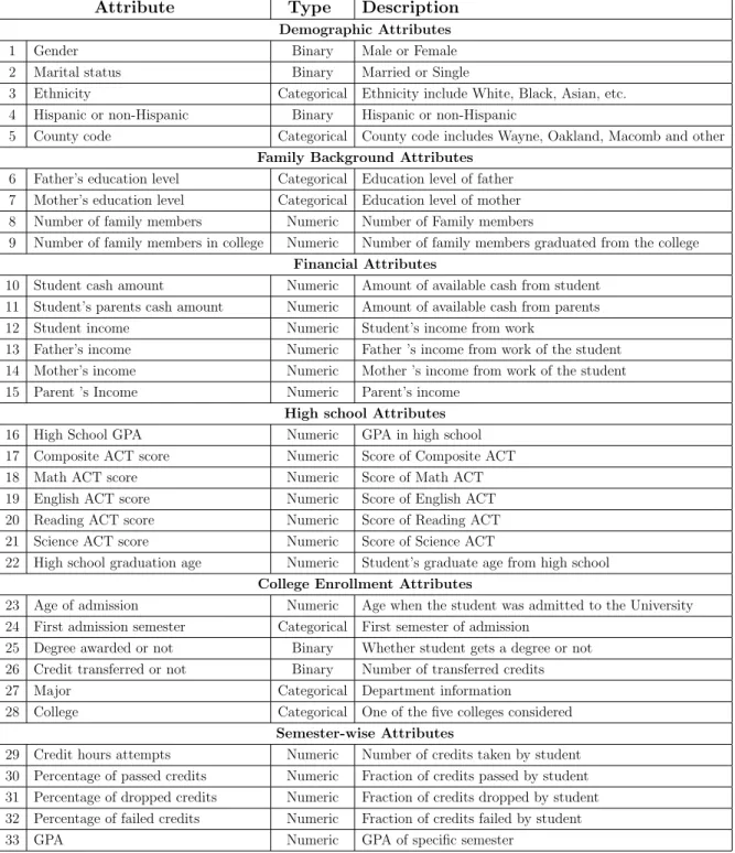
Among these categories, only Semester-wise group attributes are time-dependent and we use them further for time-dependent survival analysis. The details of all the attributes used in our analysis is summarized in Table 4.1. We will now define some of the terms that will be used in this chapter.
• Dropout Student: It is defined as a student who does not register in a semester or whose semester GPA is zero.
• Event: The student dropout before graduation is our event of interest.
• Censored: If a student does not dropout within first 6 semesters or we have no information about it, then it is defined as censored data.
• Status: It is 1 if student dropout within first 6 semesters and 0 if he continues study and never drops out in that period.
• Time: Semester in which the dropout occurred for a given student.
In order to evaluate the performance of proposed methods we run two sets of experi-ments as follows:
• Experiment 1: In this experiment, we collected the information for students who are admitted to WSU from 2002 to 2009 and keep track of their record up to first 6 semesters. The illustration of this experiment shows in Figure 3.1.
• Experiment 2: In this experiment, we are not following all the student for 6 semesters. In other words, we cut the observation at 2009, so in this case, for students who have been admitted to school in 2008, we have records for only two semesters. For a better understanding, we illustrate this experiment in Figure 4.1. As it is shown, in this experiment we have censored data before 6th semester.
Figure 4.1: An illustration to demonstrate second experiment.
4.2
Preliminary Analysis of the Data
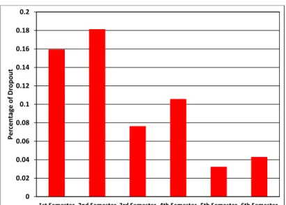
In order to have a better understanding of the WSU student retention data, in this section, we provide some descriptive analysis. Let us start with Figure 4.2 which shows the percentage of dropout in each semester. It indicates the importance of addressing dropout issue as early as possible in the student school life. From the figure, the per-centage of first year dropout is around 35% and by end of second year it increase up to 55%.
Figure 4.3 shows histogram plot for some of the important pre-enrollment attributes. It is clear that high school GPA and ACT score significantly affect the student dropout within the first 6 semesters. The higher the GPA and ACT score, the less chance of
Table 4.1: Description of attributes used to build our dataset. Attribute Type Description
Demographic Attributes
1 Gender Binary Male or Female
2 Marital status Binary Married or Single
3 Ethnicity Categorical Ethnicity include White, Black, Asian, etc. 4 Hispanic or non-Hispanic Binary Hispanic or non-Hispanic
5 County code Categorical County code includes Wayne, Oakland, Macomb and other
Family Background Attributes
6 Father’s education level Categorical Education level of father 7 Mother’s education level Categorical Education level of mother 8 Number of family members Numeric Number of Family members
9 Number of family members in college Numeric Number of family members graduated from the college
Financial Attributes
10 Student cash amount Numeric Amount of available cash from student 11 Student’s parents cash amount Numeric Amount of available cash from parents
12 Student income Numeric Student’s income from work
13 Father’s income Numeric Father ’s income from work of the student 14 Mother’s income Numeric Mother ’s income from work of the student
15 Parent ’s Income Numeric Parent’s income
High school Attributes
16 High School GPA Numeric GPA in high school
17 Composite ACT score Numeric Score of Composite ACT
18 Math ACT score Numeric Score of Math ACT
19 English ACT score Numeric Score of English ACT
20 Reading ACT score Numeric Score of Reading ACT
21 Science ACT score Numeric Score of Science ACT
22 High school graduation age Numeric Student’s graduate age from high school
College Enrollment Attributes
23 Age of admission Numeric Age when the student was admitted to the University 24 First admission semester Categorical First semester of admission
25 Degree awarded or not Binary Whether student gets a degree or not 26 Credit transferred or not Binary Number of transferred credits
27 Major Categorical Department information
28 College Categorical One of the five colleges considered
Semester-wise Attributes
29 Credit hours attempts Numeric Number of credits taken by student 30 Percentage of passed credits Numeric Fraction of credits passed by student 31 Percentage of dropped credits Numeric Fraction of credits dropped by student 32 Percentage of failed credits Numeric Fraction of credits failed by student
0 0.02 0.04 0.06 0.08 0.1 0.12 0.14 0.16 0.18 0.2
1st Semester 2nd Semester 3rd Semester 4th Semester 5th Semester 6th Semester
P er ce n tag e of Dr op ou t
Figure 4.2: Histogram plot for the percentage of dropout per semester
dropout from school. Also the gender and ethnicity could be good indicators for student at risk of dropout.
We also did an exploratory survival analysis using Coxph estimator in order to see the dropout pattern for different scenarios. Figure 4.4 shows the probability of dropout for 4 different scenarios. In each scenario, we consider all other variables which are set at average level and allow only one attribute to have a different value. As an example, in Figure 4.4(a), we test the probability of dropout for male vs. female. It is clear that gender does not have significant impact on student dropout by itself. Figure 4.4(b) shows the effect of different county residency on student dropout. It indicates that those who come from the three nearby counties have a lower chance of dropout. In Figure 4.4(c) we test the impact of different ethnicity on student dropout. Finally Figure 4.4(d) shows the importance of high school GPA on student dropout.
0 2000 4000 6000 F M Gender count Dropout NO YES (a) 0 1000 2000 3000 4000 AS BL HM HO HP UN WH Ethnicity count Dropout NO YES (b) 0 500 1000 1500 1 2 3 4 GPA_Highschool count Dropout NO YES (c) 0 500 1000 1500 2000 6 8 9 10 11 12 13 14 15 16 17 18 19 20 21 22 23 24 25 26 27 28 29 30 31 32 33 34 35 ACT_Composit count Dropout NO YES (d) 0 2000 4000 6000 8000 BA ED EN FA LS College count Dropout NO YES (e) 0 500 1000 1500 2000 2002 2003 2004 2005 2006 2007 2008 2009 Year_Admitted count Dropout NO YES (f)
Figure 4.3: Histogram plot for some of the important pre-school attributes: (a) Gender, (b) Ethnicity, (c) High school GPA, (d) ACT composite score, (e) College and (f) Year of admission
1st−sem0 2nd−sem 3rd−sem 4th−sem 5th−sem 6th−sem 0.1 0.2 0.3 0.4 0.5 0.6 0.7 0.8 0.9 1 Survival Probability Female Male (a)
1st−sem0 2nd−sem 3rd−sem 4th−sem 5th−sem 6th−sem
0.1 0.2 0.3 0.4 0.5 0.6 0.7 0.8 0.9 1 Survival Probability Wayne Okland Macomb Others (b)
1st−sem0 2nd−sem 3rd−sem 4th−sem 5th−sem 6th−sem
0.1 0.2 0.3 0.4 0.5 0.6 0.7 0.8 0.9 1 Survival Probability White Black Asian (c)
1st−sem0 2nd−sem 3rd−sem 4th−sem 5th−sem 6th−sem
0.1 0.2 0.3 0.4 0.5 0.6 0.7 0.8 0.9 1 Survival Probability GPA=1 GPA=2 GPA=3 GPA=4 (d)
Figure 4.4: Probability of attrition for 4 different variables: (a) gender, (b) county of residency, (c) ethnicity and (d) high school GPA. It should be noted that all other variables fix on an average for each case.
4.3
Evaluation Metrics
In order to have a quantitative measure of estimating the performance of the proposed model and compare with other classification techniques, we used two sets of experiments. We divide our data into training and testing sets. Training data consists of records for students who have been admitted from 2002 to 2008. Then our test data consists of student admitted in 2009 and they are completely unused during our model building. We report the results of both 10-fold cross validation on training set and the test data in separate tables. In the first one, we use standard technique of stratified 10-fold cross val-idation, which divides each dataset into ten subsets, called folds, of approximately equal size and equal distribution of dropout and non-dropout students. In each experiment, one fold is used for testing the model that has been developed from the remaining nine folds during the training phase. The evaluation metrics for each method is then com-puted as an average of the ten experiments. We also evaluate the performance of model learned using 2002 to 2008 data on the unseen test data, which is the dropout informa-tion for students who are admitted to WSU in 2009. We implemented our methods in R programming language using survival package [36] and for the rest of the methods we used open source Weka software [16]. To assess the performance of the proposed model, the following metrics are used for the classification problem.
• Accuracy is expressed in percentage of subjects in the test set that were classified correctly.
• F-measure is defined as a harmonic mean of precision and recall. A high value of
F-measure indicates that both precision and recall are reasonably high.
F −measure= 2×P recision×Recall
where P recision = T P
T P+F P and, Recall =
T P
T P+F N. T P is the true positive, F P is
false positive and F N is false negative.
• AUC is expressed as area under the a receiver operating characteristic (ROC) curve where the curve is created by plotting the true positive rate (TPR) against the false positive rate (FPR) under various threshold values.
For the time to dropout prediction which is originally a regression problem, we used following metrics:
• Mean Absolute Error (MAE) is a quantity used to measure how close the forecasts or predictions are to the actual outcomes. The mean absolute error is given by MAE = 1 n n X i=1 |yˆi−yi|
where ˆyi is the predicted value and yi is the true value for subject i.
• Root Mean Square Error (RMSE) is a frequently used measure of the dif-ferences between values predicted by a model and the values actually observed. The RMSE represents the sample standard deviation of the differences between predicted values and observed values.
RMSE =
r Pn
i=1(ˆyi−yi)2
n
• Relative Absolute Error (RAE) measures the size of the error in percentage terms as follows RAE = Pn i=1|yˆi−yi| Pn i=1|y¯−yi|
• Root Relative Square Error (RRSE) is similar to the RAE for root mean square error which can be calculated as
RRSE = s Pn i=1(ˆyi−yi)2 Pn i=1(¯y−yi)2
4.4
Performance of Various Classification Methods
In this section, we demonstrate the performance of the proposed survival analysis method, Coxph and TD-Cox, on Wayne State University student dropout information from 2002 to 2009. Table 4.2 shows the list of attributes along with their coefficients from the Coxph model. In this table, coef shows coefficients, exp(coef ) shows the exponential of each coefficient and se(coef ) is standard error of the coefficients. The
z value is the Wald statistic for testing the hypothesis that the coefficient is zero and
Pr(> |z|) is the tail area in a 2-tail test. The results show that the number of family members, number of family member at college, county of residency, age of admission to college, ethnicity, high school GPA and ACT score have a significant impact on student dropout.
We compare the performance of our proposed TD-Cox and the standard Cox method against three well-known classification techniques in the machine learning domain, namely, Logistic Regression (LR), Adaptive Boosting (AB) and Decision Tree (DT). We test the performance of the models to predict the student dropout in different semesters for the two experimental setups explained in Section 4.1. The results are shown in Tables 4.3-4.6. From these Tables, we can see the consistent results of the TD-Cox method which beat all other methods. Comparing results in Tables 4.3 and 4.4 with Tables 4.5 and 4.6, it is clear that we could get higher performance from Cox and TD-Cox (survival analysis methods) in the presence of more censored data. In this study, as described in Table 4.1, we define 5 after-enrollment variables including GPA, percentage of passed,
Table 4.2: Coefficient estimation of the attributes from the Coxph model
Attributes coef exp(coef ) se(coef ) z Pr(>|z|)
Father Edu -0.017175 0.982972 0.015994 -1.074 0.28289
Mother Edu -0.027029 0.973333 0.017743 -1.523 0.12767
No Family Member 0.094209 1.098789 0.010161 9.272 2.00E-16 No At College -0.566458 0.567532 0.024475 -23.145 2.00E-16
County Okland 0.002401 1.002404 0.044641 0.054 0.95711
County Other 0.644733 1.905478 0.061575 10.471 2.00E-16
County Wayne 0.23978 1.270969 0.03684 6.509 7.58E-11
Transfer Credit -1.009215 0.364505 0.042285 -23.867 2.00E-16
CollegeED -0.041782 0.959079 0.082031 -0.509 0.61051
CollegeEN -0.098913 0.905821 0.064003 -1.545 0.12224
CollegeFA -0.166346 0.846754 0.058515 -2.843 0.00447
CollegeLS -0.046164 0.954886 0.046968 -0.983 0.32567
GPA Highschool -0.419755 0.657208 0.031141 -13.479 2.00E-16 Age Highschool grad -0.006037 0.993981 0.011206 -0.539 0.59008
Age Enter College 0.013679 1.013772 0.003677 3.72 0.0002
Gender -0.063127 0.938824 0.027993 -2.255 0.02413 Marrital StatusS 0.004511 1.004521 0.095535 0.047 0.96234 Hispanic YES -0.829685 0.436187 0.31907 -2.6 0.00931 ETHN BL 0.291758 1.33878 0.064063 4.554 5.26E-06 ETHN HM 0.858316 2.359185 0.33363 2.573 0.01009 ETHN HO 0.875152 2.399239 0.360104 2.43 0.01509 ETHN HP 0.675308 1.964637 0.596507 1.132 0.25759 ETHN WH 0.050288 1.051573 0.06226 0.808 0.41926
ACT English -0.03331 0.967239 0.007746 -4.3 1.71E-05
ACT Math -0.014869 0.985241 0.008098 -1.836 0.06636
ACT Reading -0.018038 0.982124 0.007631 -2.364 0.01809 ACT Science -0.023999 0.976287 0.008328 -2.882 0.00396
dropped or failed credits and credit hours attempts. When we used those attributes along with pre-enrollment variables in proposed TD-Cox method, we get better classification performance. Thus, unlike other classification methods, the proposed TD-Cox approach has the ability to utilize extra semester-wise information by introducing time-dependent variables in the model.
Figure 4.5 and 4.6 provide the performance comparison between all the methods for each semester for different experimental setup. It can be observed that the accuracy and F-measure increase significantly for TD-Cox when we have more semester-wise informa-tion. The ability of TD-Cox to leverage those information provides in more accurate prediction of student dropout. We can also conclude that in the presence of censored data, survival analysis methods such as the one that is being used in this thesis (Cox and
TD-Cox) are a better choice for predicting student dropout. On the other hand, even if we rely only on the pre-enrollment attributes, Cox provides a better performance com-pared to other machine learning based classification methods. This suggests that Cox regression model would be a better choice for longitudinal data classification problem compared to the traditional methods. One important reason behind this is that it can appropriately handle censored data. Thus, it is important to note that time-dependent variables and handling censoring data are two specific features of longitudinal data that survival models such as Cox can efficiently handle. It is worth to mention that by com-paring the result of 10-fold cross validation (Tables 4.3 and 4.5) and the test data for year 2009 (Tables 4.4 and 4.6) we can observe the clear benefits of using the proposed model.
4.5
Evaluation on Predicting Semester of Dropout
One of the primary purposes of this study is to build a model to estimate the semester of dropout using only the pre-enrollment information at the beginning of the study. As discussed earlier, one of the drawbacks of using linear regression in the presence of
Table 4.3: Performance of Logistic regression, Adaboost and Decision tree with Coxph and TD-Cox on WSU student retention data from 2002 to 2008 (experiment 1) for each semester using 10-fold cross validation along with standard deviation.
Model Accuracy F-measure AUC
1st Semester Logistic 0.705 (0.023) 0.702 (0.031) 0.734 (0.015) AdaBoost 0.709 (0.019) 0.712 (0.028) 0.747 (0.013) Decision tree 0.706 (0.035) 0.7 (0.049) 0.662 (0.026) Coxph 0.719 (0.015) 0.724 (0.029) 0.751 (0.013) TD-Coxph 0.719 (0.015) 0.724 (0.029) 0.751 (0.013) 2nd Semester Logistic 0.715 (0.025) 0.715 (0.033) 0.766 (0.018) AdaBoost 0.721 (0.02) 0.724 (0.029) 0.78 (0.015) Decision tree 0.713 (0.037) 0.711 (0.051) 0.697 (0.023) Coxph 0.729 (0.019) 0.737 (0.031) 0.783 (0.012) TD-Coxph 0.765 (0.018) 0.741 (0.03) 0.792 (0.011) 3rd Semester Logistic 0.728 (0.024) 0.729 (0.034) 0.795 (0.017) AdaBoost 0.733 (0.019) 0.734 (0.033) 0.802 (0.014) Decision tree 0.723 (0.034) 0.723 (0.048) 0.727 (0.019) Coxph 0.743 (0.018) 0.744 (0.028) 0.804 (0.013) TD-Coxph 0.778 (0.016) 0.761 (0.029) 0.811 (0.012) 4th Semester Logistic 0.741 (0.021) 0.741 (0.032) 0.816 (0.016) AdaBoost 0.738 (0.027) 0.742 (0.03) 0.82 (0.015) Decision tree 0.727 (0.031) 0.734 (0.049) 0.738 (0.021) Coxph 0.747 (0.017) 0.747 (0.029) 0.831 (0.014) TD-Coxph 0.801 (0.018) 0.784 (0.027) 0.835 (0.013) 5th Semester Logistic 0.748 (0.025) 0.746 (0.034) 0.824 (0.016) AdaBoost 0.751 (0.029) 0.751 (0.031) 0.826 (0.015) Decision tree 0.734 (0.039) 0.739 (0.039) 0.755 (0.019) Coxph 0.756 (0.02) 0.754 (0.027) 0.832 (0.012) TD-Coxph 0.812 (0.019) 0.801 (0.026) 0.84 (0.012) 6th Semester Logistic 0.762 (0.028) 0.758 (0.03) 0.827 (0.014) AdaBoost 0.755 (0.023) 0.755 (0.035) 0.828 (0.016) Decision tree 0.745 (0.034) 0.742 (0.045) 0.75 (0.021) Coxph 0.767 (0.017) 0.767 (0.028) 0.836 (0.011) TD-Coxph 0.821 (0.015) 0.818 (0.024) 0.847 (0.009)