Essays in Banking and Default

Essays on Banking and Default

An¬l Ar¬

Faculty of Economics

University of Cambridge

This dissertation is submitted for the degree of

Doctor of Philosophy

Excerpt from Ithaka

Keep Ithaka always in your mind. Arriving there is what you are destined for.

But do not hurry the journey at all. Better if it lasts for years,

so you are old by the time you reach the island, wealthy with all you have gained on the way,

not expecting Ithaka to make you rich.

Ithaka gave you the marvelous journey. Without her you would not have set out.

She has nothing left to give you now.

And if you …nd her poor, Ithaka won’t have fooled you. Wise as you will have become, so full of experience, you will have understood by then what these Ithakas mean.

Declaration

This dissertation is the result of my own work and includes nothing which is the outcome of work done in collaboration except as declared in the Preface and speci…ed in the text. It is not substantially the same as any that I have submitted, or, is being concurrently submitted for a degree or diploma or other quali…cation at the University of Cambridge or any other University or similar institution except as declared in the Preface and speci…ed in the text. I further state that no substantial part of my dissertation has already been submitted, or, is being concurrently submitted for any such degree, diploma or other quali…cation at the University of Cambridge or any other University or similar institution except as declared in the Preface and speci…ed in the text. It does not exceed the prescribed word limit of 60000 words.

Anil Ari August 2017

Acknowledgements

Words are not enough to express my gratitude towards my supervisor Chryssi Giannitsarou and my research advisor Giancarlo Corsetti. It was a great privilege to learn from them. They have provided a tremendous amount of support and guidance, while still giving me the freedom to pursue my interests. Most importantly, they were great role models in showing me how to be an honest and devoted researcher. For this, I am truly indebted to them.

I am extremely grateful to Luca Dedola and Vasco Carvalho. I bene…ted greatly from their invaluable advice throughout my studies. They have shown sincere support and care for my development as a researcher, and for this I cannot thank them enough.

At the risk of leaving someone out, I thank Arpad Abraham, Luigi Bocola, Charles Brendon, Elisa Faraglia, Aytek Erdil, Daniel Garcia-Macia, Peter Karadi, Michal Kobielarz, Igor Livshits, Hamish Low, G. Kemal Özhan, Franck Portier, Sönje Reiche, Pontus Rendahl, Gabriella San-tangelo, Sriya Iyer, Flavio Toxvaerd and Alexandros Vardoulakis for useful comments and suggestions. I also thank my co-authors Matthieu Darracq-Paries, Christo¤er Kok and Dawid

·

Zochowski for giving me the opportunity to work with them.

My thanks go to the administrative and IT sta¤ at the University of Cambridge, in particular to Louise Cross, Silvana Dean, Jake Dyer and Marion Reusch.

I gratefully acknowledge …nancial support from the Cambridge-INET Institute, the Royal Economic Society and the Keynes Fund. On this note, I should thank Povilas Lastauskas for trusting me with the supervision of Wolfson undergraduates and for many stimulating conversations at Wolfson cafeteria.

I wish to thank fellow students and friends in Cambridge Axel, Farid, Hasan, Nicolas, Peng, River, Samuel, Simon and Katja for a great time together. I am particularly grateful to Alice and Tom for their support when the going got tough. On a lighter note, I had a lot of fun playing board games with Stephanie, David and John. It comes out combating pandemics and zombies is a great way to forget about the job market. I also really enjoyed Darbar, and thank Emile for signing me in all the time. Fred was a great person to be look-alikes with. His students still thank me for his extraordinary teaching. My numerous tea and co¤ee breaks with Margit and Bartek had a questionable e¤ect on my productivity but provided a great source of fun. I will miss you guys!

I spent a few months in Frankfurt as an intern at the European Central Bank and remember them very fondly. I would like to thank fellow interns Alexandra, Andreas, Codruta, Despoina, Dimitris, Gauthier, Gian, Ioana, Rali, Sandra, Madalina, Vaclav and Wildmer for making my time in Frankfurt memorable. Special thanks go to Thibaut for stimulating conversations over “beer dinners”, Donata for …nally getting me to ski, and Aurel and Christopher for always making me see the glass half full.

Thank you also to many friends and relatives back home in Cyprus and elsewhere, for reminding me that there is a world outside economics. I am grateful to my uncle Erdin and aunt Hülya for always being there for me. I regret that my late uncle Eren and grandmother Ayten, who were so kind and helpful, will not see me graduate.

Last but not least, I am deeply grateful to my parents Engin and Re…a, my brother Orhan and my girlfriend Monica for their continuous love and immense moral support. They have always supported me in my ambitions even though it all too often required sacri…ces from them. This thesis is dedicated to them.

Preface

My thesis combines work on several topics within the …elds of …nance and macro-economics, developed in three chapters. The …rst two chapters contribute to the literature on bank risk-taking, sovereign debt crises, and macroeconomic dynamics during …nancial and debt crises. The third chapter focuses on the recent growth of shadow banking and its implications for market discipline on traditional commercial banks.

In the …rst chapter, titled “Aggregate Risk and Bank Risk-Taking”, I propose a general equilibrium model in which strategic interactions between banks and depositors may lead to endogenous bank fragility and a drop in investment and output. With some opacity in bank balance sheets, depositors form expectations about bank risk-taking and demand a return on bank deposits according to their risk. This creates strategic complementarities and possibly multiple equilibria: in response to an increase in funding costs, banks may optimally choose to pursue risky portfolios that undermine their solvency prospects. In a bad equilibrium, bank lending is crowded out by risky asset purchases and weak economic fundamentals lead to a banking crisis.

I show that this model has important implications for economic vulnerability to crises to policy design. The problem of multiple equilibria arises in countries with high aggregate risk and an under-capitalized banking sector. In these countries, policy interventions in support of the banking sector face a trade-o¤ between alleviating banks’funding conditions and strengthening their risk-taking incentives. Due to this trade-o¤, liquidity provision to banks may back…re and eliminate the good equilibrium when it is not targeted. Targeted interventions have the capacity to eliminate the bad equilibrium.

In the second chapter, titled “Gambling Traps”, I analyze macroeconomic dynamics as-sociated with this framework in a dynamic general equilibrium model. I show that strategic interactions between banks and depositors may leave countries stuck in “gambling traps”after adverse shocks. In a gambling trap, high bank funding costs hinder the accumulation of bank net worth, leading to a prolonged period of …nancial fragility and an endogenously persistent decline in economic activity.

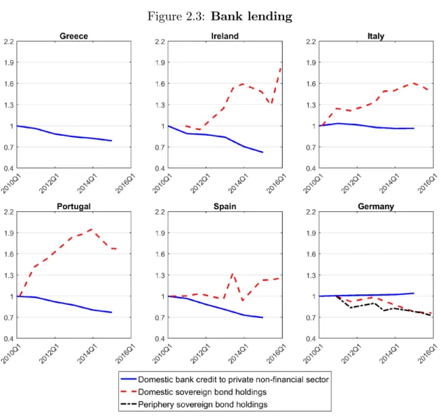
I bring this model to bear on the European sovereign debt crisis, in the course of which under-capitalized banks in default-risky countries experienced an increase in funding costs and raised their holdings of domestic government debt. The model is quanti…ed using Portuguese data and accounts for macroeconomic dynamics in Portugal in 2010-2016. Finally, I show that subsidized loans to banks, similar to the European Central Bank’s longer-term re…nancing operations (LTRO) lead to a rise in banks’ holdings of risky domestic government debt and perpetuate gambling traps.

is joint work with Matthieu Darracq-Paries, Christo¤er Kok, and Dawid ·Zochowski. In this chapter, we propose a general equilibrium banking model in which shadow banking arises endogenously and undermines market discipline on traditional banks. We show that depositors’ ability to re-optimize in response to crises imposes market discipline on traditional banks: these banks optimally commit to a safe portfolio strategy to prevent early withdrawals. When commitment is costly, shadow banking emerges as an alternative banking strategy that combines high risk-taking with early liquidation in times of crisis. We derive an equilibrium in which the shadow banking sector expands to a size where its liquidation causes a …re-sale and exposes traditional banks to liquidity risk. Higher deposit rates in compensation for liquidity risk also weaken threats of early withdrawal and traditional banks pursue risky portfolios that may leave them in default.

This theoretical model accounts for two key empirical facts about the 2007-2009 …nancial crisis in the United States: Shadow banks faced a sudden contraction in funding and the liquidation of their assets caused a …re-sale. Traditional banks did not su¤er from withdrawals, experienced a sharp rise in their funding costs, and re-allocated their portfolios towards safe and liquid assets. The model also yields novel and important insights for policy design. We …nd that policy interventions aimed at alleviating …re-sales fuel further expansion of shadow banking. Financial stability can be achieved with a tax on shadow bank pro…ts or collateralized liquidity support to traditional banks.

Contents

Declaration

v

Acknowledgements

vi

Preface

viii

1

Aggregate Risk and Bank Risk-Taking

1

1.1 Introduction 2 1.2 Model environment 6 1.2.1 Entrepreneurs . . . 7 1.2.2 Firms . . . 8 1.2.3 Households . . . 9 1.2.4 Banks . . . 10

1.2.5 Deposit demand schedule. . . 12

1.2.6 Bank strategies . . . 13 1.3 Equilibrium 16 1.3.1 Candidate equilibria . . . 17 1.3.2 Sentiments. . . 21 1.3.3 Equilibrium conditions . . . 22 1.3.4 Regions of equilibria . . . 26 1.4 Policy analysis 28 1.4.1 Liquidity provision . . . 28

1.4.2 Targeted liquidity provision . . . 31

1.4.3 Deposit insurance and macroprudential regulation . . . 32

1.5 Conclusion 34

2

Gambling Traps

35

2.2 Facts 40 2.3 Model environment 46 2.3.1 Government . . . 47 2.3.2 Firms . . . 48 2.3.3 Households . . . 49 2.3.4 Banks . . . 51

2.3.5 Sentiments and sunspots . . . 54

2.3.6 Steady state after sovereign default . . . 55

2.3.7 Equilibrium . . . 56

2.3.8 Numerical solution . . . 56

2.4 Numerical results 58 2.4.1 Calibration . . . 58

2.4.2 Sovereign risk and equilibrium regions . . . 59

2.4.3 Propagation of sovereign risk shocks . . . 61

2.4.4 Comparison with Portuguese data . . . 64

2.5 Policy analysis 66 2.6 Conclusion 67

3

Shadow Banking and Market Discipline on Traditional Banks

69

3.3.1.1 Entrepreneurs . . . 80

3.3.1.2 Secondary market and outside investors . . . 82

3.3.1.3 Households . . . 83

3.3.1.4 Banks . . . 85

3.3.2 Equilibrium . . . 89

3.3.2.1 Fire-sales and bank strategies . . . 90

3.3.2.2 Interior equilibrium . . . 91

3.4.1 Bank-runs . . . 94 3.4.2 Secondary market . . . 95 3.4.3 Analytical results . . . 96 3.5 Numerical results 97 3.5.1 Calibration . . . 97 3.5.2 Results. . . 99 3.6 Policy analysis 101 3.6.1 Asset purchases . . . 101

3.6.2 Tax on shadow bank pro…ts . . . 103

3.6.3 Liquidity provision . . . 104

3.6.4 Deposit insurance and macroprudential regulation . . . 106

3.7 Conclusion 106

Bibliography

108

Appendix

116

A2 Deviation to the safe strategy . . . 116

A3 Proofs of propositions and lemmata . . . 119

A3.1 Proof of Lemma 1.1 . . . 119

A3.2 Proof of Lemma 1.2 . . . 119

A3.3 Proof of Lemma 1.3 . . . 120

A3.4 Proof of Lemma 1.4 . . . 121

A3.5 Proof of Proposition 1.1 . . . 121

A3.6 Proof of Proposition 1.2 . . . 122

A3.7 Proof of Proposition 1.3 . . . 124

A3.8 Proof of Proposition 1.4 . . . 126

A3.9 Proof of Proposition 1.5 . . . 127

B Appendix of Chapter 2 128 B1 Liquidity Provision . . . 128

B2 Proofs of propositions and lemmata . . . 128

B2.2 Proof of Lemma 2.2 . . . 130

B2.3 Proof of Proposition 2.1 . . . 130

B3 Data and calibration . . . 132

B3.1 Sovereign default risk. . . 132

B3.2 Loan interest rates . . . 133

B3.3 Bank funding costs . . . 133

B3.4 Leverage ratio . . . 133

B3.5 Domestic sovereign bond exposure . . . 133

B4 Proofs for the numerical solution . . . 134

C Appendix of Chapter 3 137 C1 Proof of Proposition 3.1 . . . 137 C2 Limited liability . . . 138 C3 Proof of Lemma 3.1. . . 139 C4 Proof of Lemma 3.2. . . 140 C4.1 Case 1 . . . 140 C4.2 Case 2 . . . 141 C4.3 Case 3 . . . 143 C5 Solution under = . . . 143

C6 Proof for Proposition 3.2 . . . 145

C6.1 Proof for condition (C62) . . . 145

C6.2 Proof for condition (C63) . . . 147

C6.3 Proof for condition (C64) . . . 147

C6.4 Proof for condition (C65) . . . 148

C6.5 Proof for the non-emptiness of( ; ) . . . 148

C7 Proof for Proposition 3.4.3 . . . 149

C8 Example …re-sale function . . . 151

C9 Full description of the model with liquidity risk . . . 152

C9.1 Entrepreneurs . . . 152

C9.2 Banks . . . 152

C10 Alternative speci…cation for bank-runs . . . 156

List of Figures

1

Aggregate Risk and Bank Risk-Taking

1

1.3 Gambling equilbrium . . . 18

1.4 Safe equilbrium . . . 20

1.5 Sentiments . . . 22

1.6 Example with multiple equilibria . . . 23

1.7 Deviation to the safe Strategy . . . 25

1.8 Liquidity provision with risk transfer . . . 30

2

Gambling Traps

35

2.2 Bank capitalization and sovereign exposures . . . 42

2.3 Bank lending . . . 43

2.4 Loan interest rates . . . 44

2.5 Bank funding costs . . . 45

2.6 Recursive timeline . . . 46

2.7 Equilibrium Mapping . . . 61

2.8 Impulse responses to a sovereign risk shock . . . 62

2.9 Decomposition of bank lending . . . 63

2.10 Comparison with Portuguese data . . . 65

2.11 Liquidity provision . . . 67

3

Shadow Banking and Market Discipline on Traditional Banks

69

3.2 ABCP markets and shadow bank assets . . . 75

3.3 Spreads on corporate bonds . . . 76

3.4 Traditional banks during the crisis . . . 77

3.5 Timeline . . . 79

3.6 Shadow banking strategy. . . 88

3.7 Traditional banking strategy . . . 89

3.8 Fall in the secondary market price . . . 91

3.9 Numerical example . . . 93

3.10 Numerical results . . . 100

3.11 Asset purchases. . . 102

3.12 Tax on shadow bank pro…ts . . . 103

Appendix

116

B1 Domestic sovereign bond exposure. . . 134 C1 Results under alternative bank-run speci…cation . . . 156

List of Tables

1

Aggregate Risk and Bank Risk-Taking

1

1.1 Notation . . . 8

2

Gambling Traps

35

2.1 Correlation with sovereign bond yield spreads over 2010-2015 . . . 46 2.2 Calibration . . . 59

3

Shadow Banking and Market Discipline on Traditional Banks

69

3.1 Notation . . . 81 3.2 Calibration . . . 98

Chapter 1

Aggregate Risk and Bank Risk-Taking

Abstract

I propose a general equilibrium model in which strategic interactions between banks and depositors may lead to endogenous bank fragility and decline in investment and output. With some opacity in bank balance sheets, depositors form expectations about bank risk-taking and demand a return on bank deposits according to their risk. This creates strategic complementarities and possibly multiple equilibria: in response to an increase in funding costs, banks may optimally choose to pursue risky portfolios that undermine their solvency prospects. In a bad equilibrium, bank lending is crowded out by risky asset purchases and weak fundamentals lead to a banking crisis. Policy interventions face a trade-o¤ between alleviating banks’ funding conditions and strengthening risk-taking incentives. Liquidity provision to banks may eliminate the good equilibrium when not targeted. Targeted interventions have the capacity to eliminate adverse equilibria.

Keywords: Risk taking; Banking crises; Bank regulation; Financial Constraints

1.1

Introduction

Evidence from recent …nancial and debt crises shows that in response to higher aggregate risk, under-capitalized banks increase their exposure to aggregate risky assets and experience a rise in their funding costs. This leads to rising bank fragility and default risk, and raises two important questions. First, what are the circumstances and mechanism that drive banks to become excessively exposed to aggregate risk? Second, what is the role of bank funding costs? In this chapter, I propose a framework where deposits are assets priced according to their risk, and banks can optimally choose to pursue risky portfolios (which may lead to default in equilibrium) under limited liability. This creates strategic complementarities: high required deposit interest rates in anticipation of risk-taking behaviour raise the costs of funding for banks and strengthen their incentives to take on more risk. Banks may then endogenously validate depositor expectations in equilibrium, raising the possibility of multiple equilibria.

I develop my analysis by specifying a small open economy model with households, …rms, entrepreneurs, and a banking sector. Banks collect deposits from households and choose their portfolios of aggregate-risky assets and loans to …rms; households lend to banks on terms that depend on bank solvency prospects; entrepreneurs sell assets backed by a pool of risky projects; …rms invest.

Modelling the equilibrium adjustment in bank risk-taking strategies in response to funding conditions has key macroeconomic and policy implications. The kernel intuition is that, when banks are well capitalized and/or market sentiment is “good”, the resulting banking equilibrium can be described as safe. In a “safe equilibrium” banks keep their exposure to aggregate risk low. Since banks are safe, depositors accept low interest rates. With some opacity preventing depositors from observing the bank portfolio in detail, however, another equilibrium may emerge depending on the conditions of the economy and the net worth of banks. In this “gambling equilibrium”, depositors expect banks to have a high exposure to aggregate risk and hence become risky themselves. As depositors require a risk premium, banks …nd it optimal to gamble and buy risky assets. The possibility of multiple equilibria depends on bank capitalization: the problem plagues economies where the banking sector is under-capitalized.

The model naturally provides novel and important insights on the e¤ectiveness of central banks’ liquidity interventions in support of …nancial intermediaries. A key prerequisite for successful interventions is that they need to provide some risk-sharing with depositors. I show that when the repayment of o¢ cial debt takes precedence over deposits, liquidity provision is completely ine¤ective. This is because depositors anticipate the dilution of their claims to bank revenues in the event of insolvency, and raise deposit rates accordingly. The second requirement for a successful intervention is that it must be well-targeted. Non-targeted interventions that provide liquidity unconditionally face an adverse trade-o¤ between their goals of alleviating

banks’funding conditions and strengthening their incentives to gamble. When bank net worth is low, non-targeted liquidity provision may actually eliminate the safe equilibrium. In the gambling equilibrium, banks use the additional funding to increase their exposure to aggregate risk until their funding costs return to the pre-intervention level. On the contrary, targeted interventions that provide liquidity conditional on bank leverage overcome the adverse trade-o¤ and eliminate the gambling equilibrium.

These insights can be generalized to a large set of policy instruments. I show that, on its own, deposit insurance faces the same trade-o¤ as non-targeted liquidity provision (with risk sharing). A wide range of macroprudential policy instruments can be used in conjunction with deposit insurance to overcome the trade-o¤, leading to a similar outcome as targeted liquidity provision. Speci…cally, this outcome is implementable using regulatory constraints on bank liabilities or risk-weighted capital regulation.

In greater detail, I model the optimal strategies of banks and households as follows. When there is uncertainty about future economic fundamentals, bank managers adopt either a “safe” or a “gambling” strategy. The safe strategy consists of investing in a precautionary manner with the goal of remaining solvent even when fundamentals turn out to be weak. The gambling strategy consists of pursuing high exposure to risky assets, and leads to insolvency under adverse fundamentals.

Bank managers have incentives to gamble for two reasons: First, they are protected by limited liability. If fundamentals turn out to be strong ex-post, risky assets pay a high return driven by the risk premium; when fundamentals are weak, banks are shielded from the full consequences of their losses by limited liability. Second, they are subject to aggregate (i.e. non-diversi…able) risk. Bank managers anticipate (quantitatively small) costs that may hit them in the event of weak fundamentals independent of their holdings of risky assets. I model these costs as re‡ecting all balance sheet losses that a macroeconomic recession can impose on banks other than the direct impact of losses on risky assets. By way of example, a downturn usually leads to a deterioration in the value of illiquid assets and a rise in non-performing loans. To the extent that deposit insurance is incomplete and/or lacks credibility, households optimally act on their assessment of bank solvency prospects by demanding higher rates on their deposits.1 _{I …rst show that the dependence of bank solvency on deposit repayment obligations} creates a kink in the optimal deposit schedule. Above a threshold level of deposits, households anticipate that banks will become insolvent in the event of weak fundamentals and demand higher interest payments in compensation. Another determinant of banks’solvency prospects is their exposure to risky assets. The higher this exposure is, the lower the level of deposits at

1_{Deposit insurance schemes typically guarantee deposits only up to a limit (Demirguc-Kunt et al.,2008). In}

real terms, depositor losses can take the form of a suspension of convertibility and a currency devaluation as well as an explicit bail-in.

which banks become insolvent in case of default. Increasing exposure thus translates into an inward shift of the deposit threshold.

With full transparency of bank balance sheets, the anticipated tightening of the deposit threshold would deter banks from increasing their exposure to aggregate risk, and by extension, rule out a gambling strategy. However, banks are typically able to obscure the composition of their investment in a variety of ways, including reliance on shell corporations and complex …nancial instruments.2 _{I assume, realistically, that households cannot directly observe portfolio} exposures and have to form expectations about banks’strategies.

I refer to anticipations of a safe strategy as “good sentiments”, as opposed to “bad senti-ments” associated with anticipation of gambling. Since the gambling strategy revolves around higher exposure to aggregate risk, bad sentiments result in a tightening of the deposit thresh-old. Bank managers strive to satisfy a solvency constraint under the safe strategy. Any shift to bad sentiments further constrains their ability to raise funds and reduces the value of the safe strategy relative to gambling. Bad sentiments may then become self-ful…lling when the tightening of the deposit threshold makes it optimal for banks to adopt the gambling strategy. I solve for a rational expectations equilibrium and …nd that the characterization of the equilibrium outcome is contingent on bank net worth. With su¢ ciently high net worth, bank managers adopt a safe strategy regardless of the location of the deposit threshold and only positive sentiments are con…rmed in equilibrium. In this “safe equilibrium”, banks reduce risky asset purchases and deleverage to satisfy their solvency constraints, while bank funding costs remain at the risk-free rate. Conversely, only a gambling equilibrium may be sustained with su¢ ciently low net worth. In a gambling equilibrium, banks increase their exposure to risky assets at the expense of credit to …rms and bank funding costs are high. Finally, sentiments become self-ful…lling in an intermediate region of net worth. A rise in aggregate risk ampli…es the impact of sentiments on bank funding costs and expands this “multiplicity region”.

Relationship to the literature This chapter is related to the literature on bank risk-taking. The insight that limited liability and portfolio opacity lead to risk-shifting may be traced back toJensen and Meckling(1976) andKareken and Wallace(1978). Krasa and Villamil (1992) emphasize the importance of aggregate risk by showing that banks take excessive risk only when they are not able to fully diversify their portfolios. It is the combination of these three ingredients that leads to the emergence of the gambling equilibrium in this chapter.

A strand of this literature focuses on competition between banks. Keeley (1990),Allen and Gale(2000) and Hellmann et al.(2000) among many others3 develop models where imperfectly

2_{The level of deposits is public information. Although banks may also raise funds through less transparent}

methods, this has no impact on the repayment prospects of depositors due to their seniority.

3_{See alsoMarcus(1984),Suarez(1994) andMatutes and Vives(2000). Carletti(2008) provides an extensive}

competitive banks make excess pro…ts. Expected future pro…ts then create skin in the game and temper banks’ risk-taking incentives. In these studies, greater competition for deposits raises bank funding costs and reduces pro…t margins, leading to a rise in bank risk-taking. Chan et al. (1986), Besanko and Thakor (1993) and Marquez (2002) reach similar conclusions in environments where excess pro…ts stem from informational rents. Dell’Ariccia et al. (2014) propose a model where interest rate hikes lead to a rise in bank risk-taking through a similar mechanism when banks are under-capitalized.

Boyd and De Nicolo(2005) show that introducing moral hazard in loan markets may reverse these …ndings. They propose a model where increased competition among banks reduces interest rates on loans. With lower loan rates, borrowers invest in less risky projects which in turn increase asset quality and reduce bank risk. Martinez-Miera and Repullo (2010) …nd that allowing for imperfect correlation across borrowers’default probabilities weakens this channel. This chapter also proposes a model with imperfect competition where a rise in the funding costs of banks reduces their pro…t margins and increases risk-taking incentives. Di¤erent to the literature on bank competition, however, it focuses on depositor expectations about bank risk-taking as a determinant of bank funding costs. The main contribution of this chapter is to show that these expectations may become self-ful…lling: When depositors expect high risk-taking by banks, they demand a risk premium on deposits. High funding costs in turn strengthen banks’ risk-taking incentives. With su¢ ciently low bank net worth and high aggregate risk, depositor expectations become self-ful…lling such that there are multiple equilibria.

The multiplicity mechanism considered in this chapter di¤ers from bank-runs à laDiamond and Dybvig (1983) in that it pertains to banks’ ante risk-taking decisions rather than ex-post withdrawals. In the gambling equilibrium, banks invest in risky portfolios that leave them vulnerable to default risk. However, these risks only come to pass when economic fundamen-tals turn out to be weak. With strong fundamenfundamen-tals, banks remain solvent regardless of the equilibrium type.

Repullo(2004),Farhi and Tirole(2012) andAcharya et al.(2016) also propose models with multiplicity in bank risk-taking. In Repullo (2004), banks compete for deposits in a circular road model and there are multiple equilibria when the degree of competition is su¢ ciently strong. In Farhi and Tirole (2012) and Acharya et al. (2016), multiplicity stems from time inconsistency in the government’s bailout incentives. In a bad equilibrium, banks invest in a risky asset in anticipation of government support and the correlation in their exposures makes it optimal for the government to provide support. In these studies, multiple equilibria arise due to strategic complementarities across banks. In contrast, this chapter analyzes strategic complementarities between the optimal strategies of banks and depositors.

Finally, this chapter is related to the literature on the risk-taking implications of policy interventions in support of the banking sector. Many of the studies discussed above emphasize

that policy interventions face a trade-o¤ between increasing bank pro…ts under a safe portfolio strategy and providing additional opportunities for risk shifting. Cordella and Yeyati (2003) …nd that the former e¤ect dominates when interventions are contingent on adverse macroeco-nomic conditions. Marquez (2017) reach a similar conclusion when a large portion of bank investors may not observe bank behaviour. In this chapter, the latter e¤ect dominates such that deposit insurance guarantees and unconditional liquidity provision back…re and eliminate the safe equilibrium. Instead, the gambling equilibrium may be eliminated with targeted inter-ventions which provide liquidity conditional on bank leverage.

Layout The remainder of this chapter is structured as follows: Section 1.2 describes the model environment. Section 1.3 presents the equilibrium solution. Section 1.4 conducts policy analysis. Section 1.5 concludes.

1.2

Model environment

I consider a stylized model of small open …nancial economy with four agents: households, banks, entrepreneurs and …rms. Events unfold over two time periods (see Figure 1.1 for a graphical timeline). In the …rst period, banks collect deposits from households and use these funds, along with their own net worth, for asset purchases and working capital lending to …rms. Entrepreneurs issue assets backed by their investment in a pool of risky projects. Firms produce the consumption good.

In the second period, economic fundamentals turn out to be weak with (exogenous) prob-ability P. Weak fundamentals lead to a haircut on risky assets and reduce the productivity of …rms. If banks are left with insu¢ cient funds to pay the promised return to their deposi-tors, they become insolvent under limited liability and a haircut proportionate to their funding shortfall is imposed on deposits.4

Banks’solvency prospects in the event of weak fundamentals are determined by the strat-egy their managers adopt in the …rst period. The ‘safe stratstrat-egy’ consists of investing in a precautionary manner that leaves them solvent under weak fundamentals, whereas the ‘gam-bling strategy’leads to insolvency. Bank managers …nd it optimal to follow the strategy that maximizes their expected payo¤.

A key friction in the model is the limited transparency of bank balance sheets. Speci…cally, households observe the amount of deposits collected by banks but not their exposure to risky assets, which can be obscured through the use of shell corporations and/or complex …nancial

4_{The absence of safe assets among banks’ investment opportunities serves only to simplify the exposition.}

Their inclusion would be completely inconsequential in this set up as purchasing a safe asset is either equivalent to or less pro…table than a reduction in deposits by the same amount.

Figure 1.1: Timeline

instruments. This leads to a two-way relationship between the optimal strategies of bank managers and households. When households anticipate that banks follow a gambling strategy, their optimal deposit schedule changes in a manner that increases banks’incentives to gamble. Household expectations about bank risk-taking may then become self-ful…lling.

Finally, before I explain these activities in more detail, it is convenient to describe some notational conventions. Table 1.1provides a list of variables and parameters. Deposits, risky assets, loans and safe assets are respectively labelled as(d; b; l; d )and take the form of discount bonds with prices q; qb_{; q}l_{; q .}5 _{The recovery rates of (d; b; l) under weak fundamentals are}

; b; l . An underbar denotes variables at the state with weak fundamentals such that A is productivity when fundamentals turn out to be weak. Aggregate quantities, such as aggregate loans L, are in the upper case while lower case variables pertain to an individual bank.

1.2.1

Entrepreneurs

In the …rst period, entrepreneurs invest in a large pool of high-risk projects and issue assets b backed by their returns. Diversi…cation across projects ensures that asset payo¤s are contingent only on the aggregate state such that they pay a recovery rate b ₂ (0;1) when fundamentals turn out to be weak.6

Assets are internationally traded and their marginal buyers are deep pocketed foreign

in-5_{This helps simplify the exposition without any actual impact on the model mechanisms.}

6_{Note that these assets may be interpreted as any asset class with high aggregate risk. For example, they}

could take the interpretation of mortgage-backed securities in the context of the 2007-09 …nancial crisis in the United States, sovereign bonds issued by periphery countries during the Eurocrisis, or any asset denominated in domestic currency in a currency crisis.

Table 1.1: Notation Variables Label Description d Deposits b Aggregate-risky assets l Loans to …rms d Safe assets q; ql_{; q}b_{; q Asset prices} ; l; b Recovery rates H Labour supply w Wages K Working capital Y Output

n Bank net worth Bank pro…ts

v Bank expected payo¤ Exposure to aggregate risk

c Consumption

l Loans market mark-up d Deposit market mark-up

Parameters

Label Description

P Prob. of weak fundamentals Market share of banks A Productivity

Cobb-Douglas elasticity Discount factor

E Household endowment

vestors. As such, they are priced at their expected return

qb = 1 P +P b q (1.1)

where 1=q is the risk-free rate.7

1.2.2

Firms

Firms are perfectly competitive. In order to produce the consumption goodY, they hire labour H from households at a wage w and borrow working capital

K =qlL (1.2)

7_{I implicitly assume that the availability of risky projects is large relative to the size of the domestic banking}

sector. In a monetary union setting, 1=q can be interpreted as the interest rate set by the common central bank.

from the domestic banking sector. In the interest of a clear exposition, loans to …rms take the form of discount bonds L sold at a price ql. Under a standard Cobb-Douglas production function, the representative …rm’s pro…t maximization problem is

max

K;L;H;H (1 P) AK H

1

L wH +P AK H1 lL wH

subject to (1.2), whereAis productivity and lis the recovery rate of loans. Crucially, ql_{; L; K}

are not state contingent as …rms borrow in advance. When fundamentals are weak, loans become non-performing due to the productivity declineA < Aand banks claim the …rm’s revenues net of salary payments such that8

l

= AK H

1 _wH

L

Combining this with the …rst order conditions of the …rm’s problem yields the expressions

w= (1 )AK w= (1 )AK ql = 1 A 1 L1 (1.3) l = A A

where labour supply is perfectly inelastic and normalized to H = H = 1. Of particular importance are the last two expressions, which respectively establish an upward-sloping loan supply schedule and pin down the recovery rate.

1.2.3

Households

There is a unit continuum of risk neutral households with an initial endowment E. They save by purchasing safe assets D at a price q or deposits D from domestic banks at a price q.9;10

8_{This is the reduced-form outcome of a re-negotiation game between …rms and banks after loans become}

non-performing. As …rms are perfectly competitive and banks have market power, the latter extracts all of the remaining revenues after salary payments. Implicitly, this relies on the absence of information asymmetries, which can be motivated by relationship banking. This also makes it prohibitively costly for households and foreign entities to lend directly to …rms. The domestic banking sector thus acts as a …nancial intermediary that channels funds to …rms. Note that the outcome here is equivalent to the issuance of state-contingent debt by …rms.

9_{The assumption of risk neutrality only serves to attain a tractable expression for the deposit demand}

schedule. The results presented below retain their validity under risk aversion, which is introduced in a similar model in Chapter 2. Similarly, permitting households to purchase risky assets has no e¤ect on the outcome.

10_{D can be interpreted as deposits in a safe foreign bank or simply as a safe real asset. As there is a unit}

continuum of homogenous households, individual households’deposits are identical to the aggregate quantities. I abuse notation by using the aggregate terms(D; D )to describe the household’s problem.

The representative household’s utility maximization problem can be described as follows

max c1;c2;c2;D;D

u(c1) + [(1 P)u(c2) +P u(c2)]

subject to the period budget constraints

c1+qD+q D =E

c2 =D+D +w

c₂ = D+D +w

where is the rate at which households discount future consumption and is the recovery rate of domestic bank deposits under weak fundamentals. This yields the …rst order conditions

q = (1.4)

q = (1 P +P )q (1.5)

which indicate that domestic deposits are priced at their expected return relative to the safe asset. Observe that households’ valuation of domestic deposits increases in recovery rate . I provide an expression for in the next section before deriving the optimal deposit demand schedule of households in Section 1.2.5.

1.2.4

Banks

The domestic banking sector is imperfectly competitive in the manner of Cournot. Each bank is risk neutral with a market share ₂(0;1]. The representative bank …nances its risky asset purchases and lending to …rms with deposits collected from households as well as its own net worthn 0. Its budget constraint can be written as

n+qd=qbb+qll (1.6)

where l = L, d = D represent lending and deposits at individual bank level. Pro…ts are contingent on economic fundamentals as follows

= max_f0; l+b d_g (1.7)

= max 0; ll+ bb d (1.8)

where represents pro…ts in the event of weak fundamentals, and the maximum operators re‡ect limited liability. Banks always make a strictly positive pro…t under strong fundamentals

( >0) but may become reliant on limited liability after fundamentals turn out to be weak. This leads to insolvency, with losses passed on to depositors through a haircut on deposits. The recovery rate of deposits re‡ects the bank’s shortfall of funds11

= min 1;

l

l+ bb

d (1.9)

with <1 indicating that limited liability binds.

The representative bank chooses its deposits d, asset purchases b and loans l in order to maximize its expected payo¤

v = (1 P) +P

subject to the budget constraint. Note that choosing(b; l)is equivalent to selecting the share of funds ₂[0;1]spent on risky asset purchases, which I refer to as banks’exposure to aggregate risk. Using (1.6), (b; l)can be de…ned in terms of as

b = n+qd

qb (1.10)

l = (1 ) n+qd

ql (1.11)

It is convenient for the remainder of the text to express the recovery rate in terms of aggregate risk exposure

= 1 b for d d( ) qb + (1 ) l ql n d +q for d > d( ) (1.12) d( ) = b qb + (1 ) l ql n 1 q _qbb + (1 ) l ql (1.13)

whered( )represents the threshold of deposits above which the bank becomes insolvent under weak fundamentals.12 Observe thatd( )and are positively related to bank net worthn and the rate of return _qbb + (1 )

l

ql on bank funds.

Recall from the previous section that the price of depositsq increases in . Under imperfect competition, banks internalize the e¤ects of their actions on and hence q. As such, it is necessary to determine the household’s optimal deposit demand schedule in the next section before evaluating bank strategies in Section 1.2.6.

11_{There is no deposit insurance or bailot guarantees in the baseline model. These are evaluated as policy}

interventions in Section1.4.

12_{This can also be interpreted as a leverage threshold d( )=n. The claim that <1 for d > d( ) is valid}

1.2.5

Deposit demand schedule

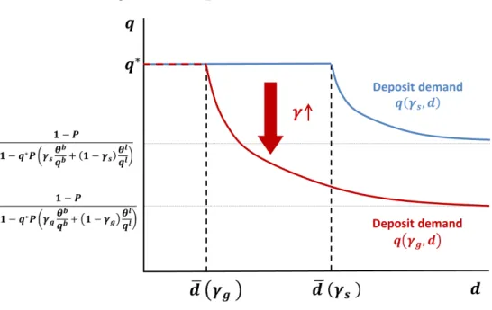
Combining (1.5) with (1.12) yields the household’s optimal deposit demand schedule contingent on q( ; d) = q for d d( ) q 1 P+P b qb+(1 ) l ql n d 1 q P b qb+(1 ) l ql for d > d( ) (1.14)

where d( ) is de…ned by (1.13). The deposit demand schedule is downward sloping and nega-tively related to under the parameter restrictions

(1 P) (1 P) + (1 ) > A A > b + (1 ) (1.15)

These restrictions ensure that following a realization of weak economic fundamentals, the rate of return from lending to …rms falls short of the promised return on deposits but exceeds that of risky assets. When the …rst inequality is satis…ed, the bank becomes insolvent under weak fundamentals given d > d( ) and the deposit demand schedule is downward sloping in this region. Therefore, I refer tod > d( ) as the ‘risky’region of the deposit demand schedule and d d( ) as the ‘safe region’. In the safe region, deposits are deemed to be risk-free with = 1 by households and priced on par with safe assets q = q . Conversely, in the risky region, households price deposits at a discountq < q in anticipation of a haircut( <1)when fundamentals turn out to be weak. At the limitd _{! 1}, the recovery rate tends to the rate of return on bank funds and the value of deposits approaches the lower bound

lim d!1q( ; d) = q 1 P 1 q P _qbb + (1 ) l ql

The second inequality in (1.15) establishes a negative relationship between the exposure to aggregate risk and the rate of return on bank funds. This ensures that the deposit threshold d( ) shifts inwards in response to a rise in , while the risky region of the deposit demand schedule pivots downward. Figure1.2shows the e¤ect of a rise in aggregate risk exposure from an arbitrary level _s to _g > _s on the deposit demand schedule.

When bank balance sheets are completely transparent, bank managers internalize the neg-ative relationship between exposure to aggregate risk and their funding conditions. Lemma1.1 shows that this imposes market discipline and deters banks from gambling on risky assets.

Lemma 1.1 When households can observe both(d; ), limited liability has no impact on banks’ optimal strategy.

Figure 1.2: Deposit demand schedule

Along with the parameter restrictions, a necessary assumption to attain the results described below is some opacity in bank balance sheets such that households can observe the amount of deposits dcollected by banks but not the aggregate risk exposure . As a result, banks cannot commit to a certain level of exposure.13

I elaborate further on the formation of household expectations on in Section 1.3.2. This discussion builds upon optimal bank strategies, however, which necessitates their explanation in advance. In the meantime, both the deposit demand schedule and the bank strategies described in the next section should be taken to be contingent on household expectations about exposure to aggregate risk, which I label as ~. Lacking commitment, banks take ~ as given and do not internalize the impact of their exposure on the deposit demand schedule q(~; d) facing them.

1.2.6

Bank strategies

Limited liability creates a discontinuity in the representative bank’s optimal strategy such that it can be evaluated as a choice between two distinct strategies. Under a ‘safe strategy’(labelled as ‘s’), the bank satis…es a solvency constraint

d ll+ bb (1.16)

which ensures that it does not rely on limited liability when fundamentals turn out to be weak. The ‘gambling strategy’ (labelled as ‘g’), on the other hand, results in the bank’s insolvency

13_{The same outcome can be attained with a timing friction whereby banks collect deposits …rst and then}

and the imposition of a haircut on deposits under weak fundamentals.

In the …rst period, the representative bank adopts the strategy that maximizes its expected payo¤ such that the safe strategy is preferred when

vs vg

where(vs; vg)are respectively the expected payo¤s associated with safe and gambling strategies.

Gambling strategy When the bank follows the gambling strategy, it solves the problem

vg = max

d; 2[0;1](1 P) (l+b d) (1.17)

s.t. n+qd = qbb+qll

where (1.10) and (1.11) map the choice of into(b; l). Since limited liability binds under weak fundamentals, the bank only internalizes the payo¤ in the state with strong fundamentals. It also internalizes the deposit demand and loan supply schedules

q q(~; d) (1.18)

ql = 1

A

1

(l+ (1 )L)1 (1.19)

given by (1.14) and (1.3) due to imperfect competition.14 The …rst order conditions can then be written as

qb = (1 _d(~; d))q (1.20)

ql = (1 _l)qb (1.21)

where d(~; d) and l are the mark-ups the bank enjoys in the deposit and loan markets due

14_{(1.19) di¤ers slightly from (1.3) as it is from the perspective of an individual bank. Lrepresents aggregate}

to its market power. They are de…ned as15 d(~; d) @q(~; d) @d d q = 0 for d d(~) P ~ b qb+(1 ~) l ql n d 1 P+P ~ b qb+(1 ~) l ql n d for d > d(~) (1.22) l (1 ) + (1 ) (1.23)

Observe that the recovery rates b; l do not feature in the …rst order conditions, since the bank does not internalize its payo¤ under weak fundamentals. I elaborate further on the consequences of this while considering the gambling equilibrium in Section 1.3.1.

Safe strategy Under the safe strategy, the bank’s problem di¤ers from its gambling counterpart in two respects. First, as the bank does not rely on limited liability, the objective function internalizes the payo¤ in both states of nature such that

vs = max

d; 2[0;1](1 P) +P

= max

d; 2[0;1]

(1 P) (l+b) +P ll+ bb d

Second, this is subject to an occasionally binding solvency constraint given by (1.16) in addition to the budget constraint. The …rst order conditions for the safe strategy can then be written as l_l+ b_{b d = 0 , 0 , d} l_l+ b_{b (1.24)} qb 1 P +P b ₊ b 1 + (1 d(~; d))q (1.25) ql = 1 P +P l ₊ l 1 + (1 l) (1 d(~; d))q (1.26)

where is the Lagrange multiplier for the solvency constraint and (1.24) is the corresponding complementary slackness condition. Compared to the gambling case, the bank has a lower valuation for both b and l since it internalizes the low payo¤ from these assets in the state with weak economic fundamentals. When l > b, however, greater value is placed on loans compared to risky assets relative to the gambling case. Both of these e¤ects are ampli…ed when the solvency constraint is binding such that >0.

The weak inequality in (1.25) re‡ects the possibility that the bank may prefer not to purchase

15_{Observe that there is no deposit market mark-up in the safe region of the deposit demand schedule. This}

is because banks face a horizontal deposit demand schedule in this region as their deposits become perfectly substitutable with safe assets.

any risky assets ( = 0), since their price is …xed at qb = 1 P +P b q as explained in Section1.2.1.16 _{Lemma1.2 describes the conditions under which (1.25) holds with equality.}

Lemma 1.2 When = 0 and q=q , condition (1.25) holds with equality and reduces to

qb = 1 P +P b q (1.27)

and there is an interior solution for b within the range

b ₂ 0;q d(~) +n q

l_l

qb (1.28)

Otherwise, there is a strict inequality and a corner solution

qb > 1 P +P

b

+ b

1 + (1 d(~; d))q

b= 0

Proof. Provided in Appendix A3.2.

This indicates that the bank only purchases a positive amount of risky assets b > 0 when the solvency constraint is slack with = 0 and bank deposits are at the safe region of the deposit demand schedule such that q=q . In this case, (1.27) shows that the bank’s valuation of risky assets is at their expected payo¤, which is equivalent to their market price given by (1.1). The bank is thus indi¤erent to the amount of its risky asset purchases within the range (1.28). On the other hand, when the solvency constraint binds ( >0) and/or bank deposits are considered to be risky (q < q ), the bank does not purchase any risky assets.

In the next section, I characterize two candidate equilibria and determine the conditions under which they are self-con…rming.

1.3

Equilibrium

I solve for a symmetric rational expectations equilibrium which requires that all optimality con-ditions and constraints of banks, …rms and households are satis…ed, and household expectations on aggregate risk exposure ~are con…rmed in the equilibrium.17 _{Section1.3.1characterizes the}

16_{Implicitly, this is a complementary slackness condition for an occassionally binding non-negativity constraint} b 0. This constraint never binds under the gambling strategy due to the higher valuation of risky assets. An equivalent constraint for lending(l 0)is also slack at all times sinceqldeclines in response to a fall inl.

17_{I abstain from mixed equilibria, as this would complicate the solution signi…cantly without yielding any}

interesting insights in addition to those provided by analyzing symmetric equilibria. Note also that the candidate equilibria described here, and the conditions under which they are valid, would remain valid even when mixed equilibria are taken into account.

candidate equilibria. Section 1.3.2 describes how households formulate their expectations ~. Section 1.3.3 provides the equilibrium conditions as well as an intuitive demonstration of the mechanism behind multiple equilibria. Finally, Section1.3.4formally characterizes the equilib-rium regions.

1.3.1

Candidate equilibria

Under rational expectations, two candidate equilibria emerge: a ‘gambling equilibrium’where household expectations of high exposure to aggregate risk in the banking sector are con…rmed by the adoption of a gambling strategy by banks, and a ‘safe equilibrium’where the opposite is true. With a slight abuse of notation, I use the labels ‘g’and ‘s’to refer to variables pertaining to the gambling and safe equilibria.

Gambling equilibrium Under the gambling equilibrium, banks follow the …rst order conditions (1.20) and (1.21). The aggregate risk exposure _g, which must be consistent with household expectations~, is determined by combining (1.20) with the deposit demand schedule (1.14). This yields

g ! 1 (1.29)

qg ! qb

where the main takeaway is the co-movement between the value of depositsqg and risky asset

prices qb_{. Note that the corner solution in}

g is due to the risk neutrality of households.18 In

Appendix A1, I show that risk aversion leads to an interior solution _{g 2} (0;1), qg 2 qb; q

while preserving the co-movement property.

The second condition (1.21) pins down the price and quantity of loans purchased by the representative bank as ql_g = (1 _l)qb (1.30) lg = ( A) 1 1 ql1 g (1.31)

where aggregate loans are given by Lg = lg= . Since the bank only internalizes asset payo¤s

in the state with strong fundamentals, a rise in the probabilityP of weak fundamentals (which reduces qb_{) leads to a decline in bank lending. This re‡ects the crowding out of bank lending} 18_{Under risk neutrality, bank deposits are priced at their expected value and the curvature of the deposit}

demand schedule is such that the mark-up d(~; d) tends to zero as deposits increase. Therefore, under a

gambling strategy, banks …nd it pro…table to issue more deposits and use the funds to purchase risky assets until their anticipated exposure approaches unity.

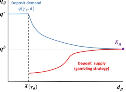
Figure 1.3: Gambling equilbrium

Note: The deposit supply curve is attained by combining (1.19 )-(1.22). Deposit demand stems from the combination of (1.14) and (1.29).

by risky asset purchases.

Finally, the expected payo¤ of banks under the gambling equilibrium is given by vg = (1 P) llg+

n

q (1.32)

where the …rst term re‡ects the mark-up from lending and the second term is the expected return on banks’initial net worth.

Figure 1.3 provides a graphical depiction of the gambling equilibrium, where the red line represents the bank’s optimal deposit supply schedule under a gambling strategy andEg marks

the equilibrium allocation.19

Safe Equilibrium Under the safe equilibrium, the deposit thresholdd( _s)coincides with the solvency constraint (1.16) such that banks always remain within the safe region of the

19_{Observe that the rate of change in the deposit supply schedule changes direction. This occurs at q}

g =

ql_g=[(1 _l) (1 _d(~; d))]. Until this point, the bank invests only in lending to …rms. By virtue of diminishing returns to scale in the production function, ql increases at an increasing rate and so does the deposit supply schedule. Beyond this point, however, the bank invests additional funds in risky assets and the deposit supply schedule is guided by (1.20). The relationship between _d(~; d)and dthen gives the schedule a positive, but decreasing rate of change that tends to zero atqg!qb.

deposit demand schedule withqs =q . The …rst order conditions can then be written as qb 1 P +P b + b 1 + q (1.33) ql= 1 P +P l + l 1 + (1 l)q (1.34)

It follows from Lemma 1.2 that there are two possible cases of the safe equilibrium, one where the solvency constraint is slack and another where it binds. Lemma1.3characterizes the safe equilibrium under both of these cases.

Lemma 1.3 There are two cases of the safe equilibrium

Case 1 Whenn nc qls q l

ls, the solvency constraint is slack( = 0)and (1.33) holds

with equality. The safe equilibrium is then characterized by20

q_sl = 1 P +P l (1 _l)q (1.35) ls = ( A) 1 1 ql1 s (1.36) bs 2 " 0;n q l s q l ls qb _q b # (1.37) ds = qb_b s+qlls n q s = qb_b s q ds+n (1.38) vs = 1 P +P l lls+ n q (1.39)

Case 2 When n < nc, the solvency constraint binds ( >0) and the safe equilibrium is

char-acterized by q lls = 1 1 ls A 1 n (1.40) ql_s = 1 A 1 ls 1 bs = s = 0 (1.41) ds = lls vs = (1 P) 1 l ls (1.42)

20_{In the de…niton forn}

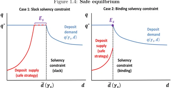
Figure 1.4: Safe equilbrium

Note: The deposit supply curve is attained by combining (1.3) with (1.34) and (1.34). Deposit demand stems from the combination of (1.14) and (1.38).

where the parameter restrictions (1.15) are su¢ cient to show that

@ls

@n >0 8 n < nc

Proof. Provided in Appendix A3.3.

Figure1.4represents the two cases graphically. In the …rst case, banks value assets according to their expected return since they do not face a binding constraint or expect to rely on limited liability. The equilibrium price of loans is then given by (1.35). As explained in section 1.2.6, banks are indi¤erent to the amount of their risky asset purchases within a range given by (1.37), because their valuation of these assets coincides with their market price. Consistent with this, there is also a range of admittable equilibrium values for(ds; s). In Figure 1.4, this is depicted

by the overlapping region Es between the deposit demand and supply curves. In order to pin

down these variables in equilibrium, I select the upper bound of (1.37) as the equilibrium value forbs. This amounts to eliminating a range of safe equilibria with lower(bs; s)values without

any impact on the characteristics of the equilibrium outcome.21

In the second case, the binding solvency constraint creates a wedge between the demand and supply of deposits. Therefore, banks do not …nd it optimal to purchase any risky assets and the equilibrium quantity of loans is implicitly de…ned by (1.40). A rise in net worth n relaxes the solvency constraint, leading to a rise in the price and quantity of loans.

Finally, it is worth discussing bank lending in the context of safe and gambling equilibria.

21_{The parameter regions under which the safe equilibrium with the selectedb}

svalue exists fully encompasses

that of safe equilibria with lowerbs values. In other words, whenever the safe equilibria with lower bs values

Proposition 1.1outlines the conditions under which a gambling equilibrium is associated with lower bank lending.

Proposition 1.1 Bank lending is lower in a gambling equilibrium under the conditions

l _> b n > 1 1 lg A 1 q llg

Proof. Provided in Appendix A3.5.

The …rst condition pertains to banks’risk-taking incentives. In a gambling equilibrium, an adverse change in economic fundamentals drives the banking sector into insolvency. Because of limited liability, banks then cease to internalize their revenues in the state with weak funda-mentals. When the recovery rate of loans exceeds that of risky assets, this leads to the crowding out of bank lending by risky asset purchases.

In spite of this, bank lending is higher under the gambling equilibrium when net worth falls short of the level required to satisfy the second condition. In this case, a tight solvency constraint forces banks to reduce their lending below the gambling level in order to ensure their solvency under weak fundamentals. Note that as the recovery rate l of loans increases, the second condition is satis…ed at a wider range of net worth, while crowding out e¤ects get stronger.

1.3.2

Sentiments

Recall from Section1.2.5that banks’aggregate risk exposure is unobservable. Nevertheless, it is a key determinant of their solvency prospects and hence the optimal deposit demand schedule q( ; d). In this section, I describe how households formulate their expectations ~ about banks’ exposures to aggregate risk. This is equivalent to forming an expectation about bank strategies since (1.29), (1.38) and (1.41) establish a one-to-one mapping between the two conditional on the observables (n; d).

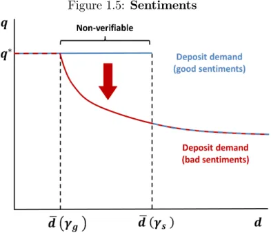
Figure 1.2 shows the deposit demand schedules associated with the expectation of safe (~ = _s) and gambling (~ = _g) strategies. Observe that households may infer the bank strategy from the level of deposits d when it lies outside the range d ₂ (d _g ; d( _s)]. When d d _g , banks remain solvent under weak fundamentals even when their exposure is at a level associated with the gambling strategy. As such, banks cannot possibly follow a gambling strategy when their deposits remain within this region. Similarly, even the low exposure s

associated with the safe strategy leads to insolvency when deposits exceed d( _s) such that d > d( _s) is not consistent with a safe strategy.

Figure 1.5: Sentiments

In contrast, within the ‘non-veri…able’ region d ₂ (d _g ; d( _s)], it is not possible to de-duce the bank strategy from observables. Expectations about the aggregate risk exposure ~

are instead determined by household sentiments such that ‘good sentiments’ refer to the ex-pectation of a safe strategy and ‘bad sentiments’refer to that of a gambling strategy. Figure 1.5 displays the deposit demand schedule under each type of sentiments. As I solve for a rational expectations equilibrium, sentiments can only exist when they are self-con…rming in equilibrium.

1.3.3

Equilibrium conditions

Under the rational expectations equilibrium framework described in section1.3.1, the safe equi-librium exists when the representative bank …nds it optimal to follow a safe strategy provided that there are good sentiments and other banks also follow a safe strategy. This leads to the equilibrium condition

vs vgjs (1.43)

where vs is the representative bank’s expected payo¤ in the safe equilibrium given in Lemma

1.3 and vgjs is the expected payo¤ from a ‘deviation to the gambling strategy’. I refer to vgjs

as a deviation payo¤ since it describes the expected payo¤ from adopting a gambling strategy when sentiments and other banks’strategies are consistent with a safe equilibrium.

Similarly, the gambling equilibrium exists under the equilibrium condition

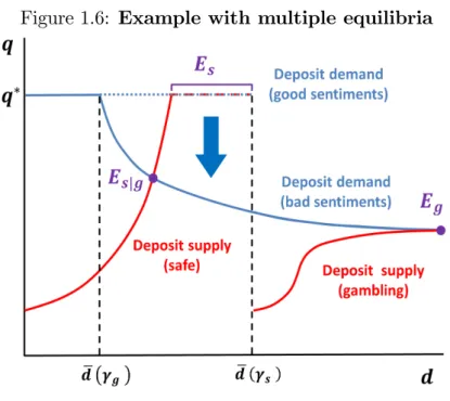
Figure 1.6: Example with multiple equilibria

where vg is the expected payo¤ under the gambling equilibrium given by (1.32) and vsjg is the

expected payo¤ from a ‘deviation to the safe strategy’. I elaborate further on these deviations below.

There are three possible equilibrium outcomes. When (1.43) is satis…ed and (1.44) is not, banks follow a safe strategy regardless of household sentiments and there is a unique safe equilibrium. In this case, bad sentiments are not self-con…rming and thus may not exist. In contrast, when (1.44) is satis…ed and (1.43) is violated, there is a unique gambling equilibrium and only bad sentiments exist. Finally, when both conditions are satis…ed, banks follow a safe strategy under good sentiments and gamble under bad sentiments such that there are multiple equilibria.

I use Figure 1.6as an informal example to provide further intuition about the mechanism behind multiple equilibria. In the interest of a clear exposition, I focus on a case where the solvency constraint remains slack regardless of household sentiments.22 _{Under good sentiments,} the representative bank faces the deposit demand schedule depicted by the dotted line, where the deposit threshold d( _s) is consistent with a safe strategy. This permits the bank to raise su¢ cient deposits to satisfy its optimality condition for lending (1.35) without reducing the price of its deposits below the risk-free level q under a safe strategy. It then …nds it optimal to adopt a safe strategy such that there is a safe equilibrium Es and good sentiments are

con…rmed.

22_{This mechanism becomes even stronger when the solvency constraint binds, since the downward pivot in}

the deposit demand schedule under bad sentiments leads to a tightening of the solvency constraint as shown in the third panel of Figure1.7.

When there is a shift to bad sentiments, the expectation of a high aggregate risk exposure

g > sleads to an inward shift of the deposit threshold tod g < d( s). The deposit demand

schedule then pivots downward in the non-veri…able regiond₂(d _g ; d( _s)]. Because of this deterioration in the bank’s borrowing conditions, the quantity and price of deposits fall to Esjg under the safe strategy. This leads to a decline in the expected payo¤ associated with

this strategy. If the bank …nds it optimal to deviate to a gambling strategy that leads to the outcomeEg, bad sentiments are also con…rmed and there are multiple equilibria.

Below, I brie‡y describe the deviations to gambling and safe strategies before characterizing the parameter boundaries for the three equilibrium regions (with a unique safe equilibrium, a unique gambling equilibrium, and multiplicity) in Section 1.3.4.

Deviation to the gambling strategy Consider a deviation to the gambling strategy when sentiments and other banks’ strategies correspond to the safe equilibrium in Section 1.3.1. Under such a deviation, the bank’s strategy is guided by the …rst order conditions (1.20) and (1.21), yielding valuations for deposits and loans that are consistent with a gambling equilibrium.

However, the quantity of loans purchased by the deviating bank lgjs= qgl

1 _{( A)1}1 1 _l

s (1.45)

di¤ers from its gambling equilibrium counterpart, which is given by (1.31). This is because the remaining banks each purchase an amount ls consistent with the safe equilibrium, thus

driving up loan prices. The negative relationship between lgjs and ls follows directly from the

upward-sloping loan supply schedule. As other banks provide more loans, the scope for lending by the deviating bank diminishes. This also reduces the expected payo¤ from deviation which is increasing in bank lending as in the gambling equilibrium

vgjs = (1 P) llgjs+

n

q (1.46)

Lemma1.4builds upon this intuition to show that the safe equilibrium is always satis…ed when the solvency constraint is slack.

Lemma 1.4 The parameter restrictions given by (1.15) are su¢ cient to show that

vs > vgjs 8 n nc Proof. Provided in Appendix A3.4.

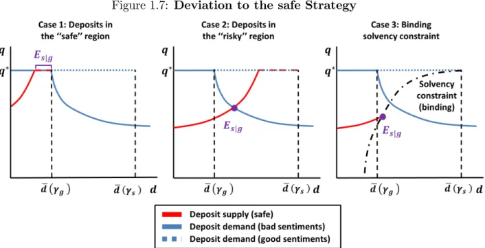
Figure 1.7: Deviation to the safe Strategy

Note: Deposit demand is attained by combining (1.14) with (1.38) under good sentiments and (1.29) under bad sentiments. The deposit supply curve stems from the combination of (1.3), (1.25), (1.26) and (1.47). The solvency constraint is given by (1.48).

binds. It is thus possible for (1.43) to be violated at a level of net worth belowncsuch that there

is a unique gambling equilibrium. I elaborate further on this in Section 1.3.4 after describing deviations to the safe strategy.

Deviation to the safe strategy Under a deviation to the safe strategy, the bank follows the …rst order conditions (1.24)-(1.26) but faces a deposit demand schedule

q _g; d = q for d d g qb ₊ P b 1 P n d for d > d g (1.47) d _g = b qb b_q n

consistent with bad sentiments. As the bank’s actual aggregate risk exposure diverges from household expectations, the solvency constraint no longer corresponds to the deposit threshold d _g . This opens up the possibility that the bank may move to the risky region of the deposit demand schedule despite satisfying the solvency constraint.

There are thus three possible cases of the deviation to the safe strategy which are valid at di¤erent regions of bank net worth n. In the interest of brevity, I relegate the characterization of these cases to Appendix A2 and instead provide a brief description of each case with the aid of Figure 1.7. In the …rst case, the deviating bank has a slack solvency constraint and

remains in the safe region of the deposit threshold dsjg d g . This case is nearly identical

to Case 1 of the safe equilibrium, except for a rise in the boundary level of net worth required for this case to be valid to nrjg > nc due to the inwards shift of the deposit threshold under

bad sentiments.23

In the second case, the shift to bad sentiments leaves the optimal level of deposits in the “risky” region of the deposit demand schedule, while the actual solvency constraint remains slack. The decline in the value of deposits to qsjg < q leads to a fall in bank lending and

expected payo¤. Finally, in the third case, the solvency constraint binds, creating a wedge between deposit demand and deposit supply and further reducing lending and expected payo¤. Note that the solvency constraint, which is given by

ql_sjg q _g; dsjg l lsjg =n (1.48)

tightens in response to a decline in the price of deposits.

1.3.4

Regions of equilibria

There are three possible equilibrium outcomes to the model. First, there is a unique gambling equilibrium when banks follow a gambling strategy regardless of household sentiments. Second, there are multiple equilibria if banks adopt a safe strategy under good sentiments and a gambling strategy under bad sentiments such that both good and bad sentiments are self-ful…lling. Third, there is a unique safe equilibrium when banks follow a safe strategy regardless of household sentiments. I denote the regions of parameters where these outcomes are prevalent as _G, _M and _S respectively.

Proposition1.2expresses the equilibrium conditions (1.43), (1.44) as parameter boundaries for these regions.

Proposition 1.2 Under the parameter restrictions given by (1.15), the mapping of equilibrium regions across net worth n is given by

E (n) = 8 > > > < > > > : G if n n Mif n < n < n S if n > n (1.49)

23_{See AppendixA2for a de…nition forn}

where n < nc is implicity de…ned by the expression n = 1 1 0 @ 1 A q (1 P) _l ql g 1 _{(A )}11 _+n q (1 P)h1 l+ _l1 i 1 A 1 (1.50) lq (1 P) l qgl 1 (A ) 1 1 +n (1 P)h 1 l + _l1 i and n is given by n (1 P)q P h (1 P) +P l(1 ) 1 P +P l 1 1 i ₍₁ l)q b 1 _{( A)1}1 l (1.51) under the su¢ cient conditions ₂(0;1₂], ₂(0;1₂].

Proof. Provided in Appendix A3.6.

Note that (1.49) indicates a monotonic ordering of equilibria across bank net worthn. Since n < nc, there is no overlap betweenMand the case of the safe equilibrium with a slack solvency

constraint. Without an upper bound to bank net worth n, this is su¢ cient to show that _S is non-empty. Proposition 1.3describes the conditions under which _fG;_Mg are also non-empty.

Proposition 1.3 Under the parameter restrictions given by (1.15), the non-emptiness of re-gions _fG;_Mg depends on where l stands with respect to the boundary l, which is implicitly de…ned by the expression

(1 ) + 1 l l = (1 l) 1 P +P b l !₁ (1.52)

There are two possible cases.

Case 1 If l l, _G is empty and _M is always non-empty.

Case 2 If l < l, _G is non-empty and a su¢ cient condition for _M to be non-empty is

b

+ (1 ) >1 P +P

b

(1.53)