A factor model for joint default probabilities. Pricing of CDS,
index swaps and index tranches
Article (Accepted Version)
Cantia, Catalin and Tunaru, Radu (2017) A factor model for joint default probabilities. Pricing of CDS, index swaps and index tranches. Insurance: Mathematics and Economics, 72. pp. 21-35. ISSN 0167-6687
This version is available from Sussex Research Online: http://sro.sussex.ac.uk/id/eprint/89499/ This document is made available in accordance with publisher policies and may differ from the published version or from the version of record. If you wish to cite this item you are advised to consult the publisher’s version. Please see the URL above for details on accessing the published version.
Copyright and reuse:
Sussex Research Online is a digital repository of the research output of the University.
Copyright and all moral rights to the version of the paper presented here belong to the individual author(s) and/or other copyright owners. To the extent reasonable and practicable, the material made available in SRO has been checked for eligibility before being made available.
Copies of full text items generally can be reproduced, displayed or performed and given to third parties in any format or medium for personal research or study, educational, or not-for-profit purposes without prior permission or charge, provided that the authors, title and full bibliographic details are credited, a hyperlink and/or URL is given for the original metadata page and the content is not changed in any way.
A Factor Model for Joint Default Probabilities. Pricing
of CDS, Index Swaps and Index Tranches
Catalin Cantiaa, Radu Tunarua,∗
aBusiness School, University of Kent, Park Wood Road, Canterbury CT2 7PE, UK
Abstract
A factor model is proposed for the valuation of credit default swaps, credit indices and CDO contracts. The model of default is based on the first-passage distribution of a Brownian motion time modified by a continuous time-change. Various model specifications fall under this general approach based on defining the credit-quality process as an innovative time-change of a standard Brownian motion where the volatility process is mean reverting L´evy driven OU type process. Our models are bottom-up and can account for sudden moves in the level of CDS spreads representing the so-called credit gap risk. We develop FFT computational tools for calculating the distribution of losses and we show how to apply them to several specifications of the time-changed Brownian motion. Our line of modelling is flexible enough to facilitate the derivation of analytical formulae for conditional probabilities of default and prices of credit derivatives.
Keywords: time-change, mean-reverting process with jumps, CDS pricing,
credit index pricing, tranche pricing
JEL: G12, C51, C63
A Factor Model for Joint Default Probabilities. Pricing of CDS, Index Swaps and Index Tranches
1. Introduction
One of the most blamed financial instruments in the aftermath of the subprime crisis is the Collateralized Debt Obligation (CDO), largely asso-ciated with the last financial crisis. Next to it, the Gaussian copula model for pricing CDOs is argued to be the formula that killed1 the Wall-Street (MacKenzie and Spears, 2014). Due to this unfavourable perception of the instrument and tougher regulation, the issuances of such instruments were greatly diminished during and after the crisis. However, most of the negative consequences associated with this instrument are born from a lack of un-derstanding and misuse combined with simplistic modelling approaches. We argue that the instrument itself has many merits and, if used and understood properly, it can improve diversification, customised risk transfer and hedging for credit portfolios.
While the subprime crisis affected negatively the issuances of CDOs, there are still important outstanding CDO contracts on the market that were issued before 2007 and that need to be properly evaluated. The low interest rate levels revived the interest of investors into the CDO market which responded with a substantial increase2 of issuances both in Europe and US.
1It was the article “Recipe for Disaster: The Formula that Killed Wall Street” from
February 2009 issue of Wired Magazine which popularized first this idea.
2See the Online Appendix for the total value of outstanding CDOs and the volumes of
Given the renewed interest in this class of instruments there is a need for further improvements to the current models for credit risk and especially portfolio credit risk. In this paper, we aim to propose a modelling methodol-ogy that allows pricing of single-name credit contracts such as credit deriva-tive swaps as well as multi-name contracts such as credit indices, tranches of a credit indices or CDOs. Investment banks routinely have to manage positions in both categories of credit instruments and managing portfolio credit risk requires the ability to calibrate on the individual components of the portfolio. Important recent contributions to credit risk modelling are Blanchet-Scalliet et al. (2011), Hurd and Zhou (2011), Cont and Minca (2013), Gatarek and Jab lecki (2013), Packham et al. (2013), Kijima and Siu (2014), Ballestra and Pacelli (2014), Hao and Li (2015) and Wei and Yuan (2016).
The evolution of credit spreads for individual obligors and portfolio of obligors may be influenced by idiosyncratic effects as well as contagion sec-tor or industry effects, and also economy wide events. Thus, several su-perimposed layers of information may determine the ebbs and flows of credit spreads. There is a clear empirical evidence that credit spreads exhibit jumps, see Dai and Singleton (2003), Tauchen and Zhou (2011), Zhang et al. (2009) and Schneider et al. (2010). These jumps are mostly positive being caused by the arrival of bad news and they impact CDS contracts across all maturities. Therefore, using L´evy processes will allow us to capture these jump effects. Early research modelling the credit quality process as a jump-diffusion or a L´evy process, see Baxter (2007) and Cariboni and Schoutens (2007), was hindered by the fact that computing first passage times was either intractable or computationally very demanding. Hao et al. (2013) obtained an analytical
formula for the survival function and also for the single-name CDS and they showed why the par CDS spread is not negligible at very short maturities.
Our main contribution is an improved credit risk model that works well with single-name contracts as well as with multi-name contracts. Our tech-niques are based on defining the credit-quality process as an innovative time-change of a standard Brownian motion where the volatility process is mean reverting L´evy driven OU type process. The factor model we propose for the evolution of probability of default for single-names is a bottom-up ap-proach to model the evolution of credit portfolios. Packham et al. (2013) conceptualised the default of a company as the first-passage time of a pro-cess modelling the credit worthiness of the company, being able in this way to capture credit gap risk and to provide an intuitive understanding of the hedging. We develop in this paper a multivariate extension, preserving the properties of the univariate model while adding the capability of modelling the time evolution of dependence between the defaults of different obligors, which is important for pricing multi-name credit contracts.
Our second contribution is to improve the computational tools that are necessary to calculate the distribution of losses at given maturity. Our FFT approach is better suited for this type of calculations than Panjer recursion and it applies to several specifications for the time-changed Brownian motion. We are also able to derive analytical formulae for conditional probabilities of default and credit derivatives. The advantage here is that one can investigate easily the sensitivity of our formulae to various model parameters. This is not always possible in general with all credit risk models, see Cont and Savescu (2008) and Bielecki et al. (2010), where numerical methods are required.
The remaining of the article is structured as follows. The modelling set-up is described in Section 2. In Section 3 we derive the formulae for default probabilities and portfolio loss. A particular feature of our modelling, the volatility of the credit quality process, is discussed in Section 4. The credit derivatives prices formulae are detailed in Section 5 while the calibration is exemplified in Section 6. Last Section summarizes our findings.
2. Default modelling
In this section we propose a factor extension for the model of default of a company proposed in Packham et al. (2013). The default is represented as the first passage time of a time-changed BM. The location of the BM rep-resents the credit quality of the company while the time-change models the arrival of information on the market that are relevant for the survival of the company. The model has the capability of modelling credit gap risk, being useful for pricing exotic credit derivative contracts and provides an intuitive understanding of the hedging. The multivariate extension of the model, pro-posed in this section, maintains the properties of the univariate model while adding the capability of modelling the time evolution of dependence between the defaults of the names in the portfolio by introducing a common factor driving the arrival of information affecting all names, which is important for pricing multi-name credit derivative contracts.
2.1. Informational setting
We consider an economy represented by a stochastic basis (Ω,F,F,P) where P is a risk neutral probability measure. In order for our model to be
well defined and to reflect reality, the filtration F= (Ft, t≥ 0) has a multi-structure design. First, we have the sub-filtration B = (Fθ, θ ≥ 0) which is the filtration of a (possibly multivariate) Brownian Motion (BM) Bθ. The second sub-filtration H= (Ht, t≥0) is incorporating information about the common factor {Ht}t≥0, and the last sub-filtration G = (Gt, t ≥ 0) is the filtration incorporating information about the idiosyncratic name specific factors {Gi
t}t≥0 where i denotes the namei. Hence, F=B∨G∨H and we
assume that all processes defined below are adapted with respect to at least one of the sub-filtrations above.
2.2. Default model
For modelling the default of companies in a portfolio ofNobligors we start with three mutually independent processes {Bt}t≥0, {ΣGt }t≥0 and {ΣHt }t≥0,
where the first two processes are N-dimensional and the last one is a uni-dimensional process.3 The process B is a standard Brownian Motion (BM)
with independent components, while ΣG and ΣH are positive processes. For any t ≥ 0 we define ΣΓ
t = ΣGt +βΣHt , with β a vector of factor loadings. Now, using B and ΣΓ we can define the credit quality process{Xt}t≥0 as the
stochastic integral: Xt= Z t 0 ΣΓsdBs= Z t 0 ΣGsdBs+β Z t 0 ΣHs dBs. (2.1)
3Other combinations are possible where more factors are considered or homogeneous
The default probabilities are driven not only by the location of the Brow-nian motion but also by the level of volatility4. In order to capture this salient feature of the credit quality process one key insight in our modelling is expressing Xt as a time changed BM:
Xt=WΓt =WGt+βHt (2.2)
where {Wθ}θ≥0 is a BM on the scale θ and Γt is a continuous time change;
Γt = Z t 0 ΣΓsds = Z t 0 ΣGsds+β Z t 0 ΣHs ds = Gt+βHt (2.3)
The two processes G and H are integrated variance processes5 and they
capture the impact of company specific and respectively market specific in-formation on the volatility of the credit quality of the names in the portfolio. Due to the common factor Hthe credit quality processes in the portfolio will move together when the market information creates volatility movements, generating dependence between the credit quality of the names.
Given the credit quality process X and its representation as a time changed BM we model as in Packham et al. (2013), henceforth the (PSS) model, the univariate default as a first-passage time over a fixed barrier bn
with n = 1,2, . . . , N of the individual credit quality process {Xn
t}t≥0, where
4We thank an anonymous referee for indicating this improved explanation.
5Note that the mutual independence assumed betweenB, ΣGand ΣHimplies that also
W, GandH are mutually independent (see Thm. 2.6 of Barndorff-Nielsen and Shiryaev
(2010)). Moreover, the processesW,GandH are adapted to the filtrationsB,GandH
τn = inf{t ≥ 0 : Xtn ≤ bn}. Our first result gives the individual probability of default.
Proposition 1. For the model described above the probability of default is
given by the formula
P(τn < s|Ft) =E 2N bn−Xtn p Γn s −Γnt Ft (2.4) The proof is almost identical to the proof of Proposition 3.3 in Packham et al. (2013) with the exception of the way condition on the filtration for the volatility takes place.
The above default model can be characterized as a hybrid “first passage time model” where the default mechanism relies on the first passage of a BM formula as in the Merton’s structural model. However, Xtn and bn are not interpreted as asset and debt level of the company, which are assumed to be unobservable. Given the representation of the credit worthiness process as a time-change BM, employing the common volatility factors to introduce de-pendence in the multivariate context becomes the obvious choice and it brings economical interpretation as well as computational tractability to the multi-variate model. The factors drive the uncertainty from various sources which adversely affects the probability of survival of a certain company (higher volatility implies less probability of survival). The formula (2.3) is similar to the one obtained in Hurd (2009) where a more relaxed definition of the first passage time of a time-changed BM is adopted. Due to this similarities, the multivariate extension discussed in this paper can be easily extended to such models.
3. Probability of Default and Portfolio Loss 3.1. Computation of Univariate Probability of Default
Without loss of generality we drop n from the notation Gn
t, τtn and bn when we only refer to one specific name. The default probability can be expressed as P(τ < s|Ft) = E E 2N b−Xt √ Γs−Γt Ft∨ Gs∨ Hs Ft = Z R+ Z R+ 2N b−Xt √ Gs+βHs−Gt−βHt PGs(dz)PHs(dy)
The computation of this probability requires the existence of closed form formulae for the densities of Gs and Hs, which are usually not available.
For the special case where the credit worthiness process{Xt}t≥0 is driven
by a Compound Poisson process as the Background Driving L´evy Process (BDLP), see definition later in Section 4), one can use Panjer recursions to compute the probability ofGsandHs and then approximate the integrals by some quadrature methods as described in Packham et al. (2013). However, this approach does not work for more general processes of the variance and hence, we propose here a faster and more general technique based on the Fourier transform. Fast computational methods are an imperative require-ment for multi-name credit derivatives, like derivative contracts on credit indices which have regularly more than 100 names in their structure (iTraxx for example has 125 names).
ex-pressed in terms of a standard normal variable Z: P(τ < s|Ft) = E[2P(Z p Γs−Γt−(b−Xt)≤0|Γs)|Ft] = E[2P(Y −K ≤0|Hs, Gs)|Ft] = E[2P(V ≤0|Hs, Gs)|Ft] (3.1) where Z ∼N(0,1), Y =Z√Gs−Gt,K =b−Xt and V =Y −K .
Since we are interested only in companies that are not in default at the time of computation of the probabilities of default, we focus on the case where the credit worthiness processX starts from above the barrier b, which implies that initiallyK <0. The characteristic function ofV is justφV(u) =
E[eiu(Y−K)|Ft] = e−iuKφY(u) and the characteristic function of Y can be calculated analytically as φY(u) = E[eiuY|Ft] =E[eiuZ √ Γs−Γt|F t] = E[E[eiuZ √ Γs−Γt|G s∨ Hs]|Ft] = E exp − u 2(Γ s−Γt) 2 Ft = eu2Γt/2 E exp − u 2 2 Γs Ft = eu2Γt/2φ Γs(−u 2/2) = eu2(Gt−βHt)/2φ Gs(−u 2/2)φ Hs(−βu 2/2) (3.2)
whereφGt(u), the moment generating function ofGt, andφHt(u), the moment
generating function of Ht, are assumed to have analytical expressions. The computation of the portfolio loss requires the computation of the probability of default conditional on the factor Hs. The conditional (on the factor Ht) characteristic function can be obtained by observing that Hs is a known
value: φY|H(u) = eu 2Γ t/2 E exp − u 2 2 Γs Ft = eu2(Gt−βHt)/2 E exp − u 2 2(Gs−βHs) Ft = eu2(βHs+Gt−βHt)/2φ Gs(−u 2/2) (3.3)
By inverting (3.3) and integrating with respect to the distribution of the fac-tor Ht one can obtain the probability of defaultP(τ < s|Ft). However, while the conditional characteristic function (3.3) has a simple form, its inversion leads to a Laplace transform which is known to be difficult to implement and expensive to evaluate (Epstein and Schotland, 2008). Therefore, we advocate using a simple Fourier inversion implementable by Fast Fourier Transform algorithms possible due to the representation in the following proposition.
Proposition 2. Given the multivariate default model described in section
2.2, any single name conditional probability of default given the factor Hs
can be computed as : P(τ < s|Hs∨ Ft) = E P 1 (b−Xt)−2Υ −(Gs−Gt)−β(Hs−Ht)≤0 Hs∨ Ft . = E[P(Q≤0)|Hs∨ Ft] (3.4)
where Υ is a chi-squared variable.
Proof. See Appendix A.
3.2. Inversion formulae
If both φGt(u) and φHt(u) are known the probability of default (and the
characteristic functions. This can be done in three ways. The first6 is the
Gil-Pelaez formula (Gil-Pelaez (1951)) for the cumulative distribution which in our context gives:
FQ(q) = 1 2+ 1 π Z ∞ 0 eiuqφQ(−u)−e−iuqφQ(u) 2iu du
To get P[Q≤0] we need to evaluate FQ(q) at zero and obtain:
P[Q≤0] = 1 2 + 1 π Z ∞ 0 eiuqφQ(−u)−e−iuqφQ(u) 2iu du = 1 2 + 1 π Z ∞ 0 eiu×0φ Q(−u)−e−iu×0φQ(u) 2iu du = 1 2 + 1 π Z ∞ 0 φQ(−u)−φQ(u) 2iu du (3.5) Because φQ(u) = φQ(−u) and <( φQ(u) iu ) = φQ(u)−φQ(u) 2iu : P[Q≤0] = 1 2 + 1 π Z ∞ 0 φQ(−u)−φQ(u) 2iu du = 1 2 − 1 π Z ∞ 0 < φQ(u) iu du
This method has the disadvantage that the above integrand has a singu-larity at zero which could create numerical problems. Since the singusingu-larity is at the lower limit of the integration domain this can be dealt with by choosing the lower limit close enough to zero.
A second useful formula has been described in Kim et al. (2010). Using that FX(x) = e xρ π < R∞ 0 e −iux φX(u+iρ) ρ−iu du implies that: P Q≤0 = 1 π< Z ∞ 0 φQ(u+iρ) ρ−iu du (3.6)
The advantage of the above formula over (3.6) is the lack of singularity given by division by zero but care is needed especially when dealing with the evaluation of the exponential function at high negative powers.
A third formula is from Feng and Lin (2013) and it is based on the Hilbert transform representation of a cumulative distribution function, expressed as a Cauchy principal value integral, H(f(x)) = π1p.vR
R
f(y)
x−ydy and exploit the relation between the Hilbert and Fourier transform F(·):
F(1(−∞,l]f)(η) = 12φQ(η)− 2ieiηlH(eiulφQ(u))(η) (3.7)
in order to write the probability distribution as:
P(Q≤0) = Z 0 −∞ pQ(x)dx= Z R 1(−∞,0)pQ(x)dx = Z R 1(−∞,0)eix0pQ(x)dx=F(1(−∞,0]f)(0) = 1 2φQ(0)− i 2e i00 H(eiu0φQ(u))(0) = 1 2− i 2H(φQ(u))(0) (3.8)
where the known relation φQ(0) = 1 is used. An approximation of Hilbert transform as a truncated infinite series is available in the form:
H(f(x)) ≈ M X m=−M f(mh)1−cos(π(x−mh)/h) π(x−mh)/h
for a step size h >0 and M a large positive integer.
All three formulae of the probability distribution above lead to Fast Fourier Transform implementation of the conditional probability of default which we summarise in the following proposition:
Proposition 3. The conditional probability of default formula in Proposition 2 has the following alternative representations with direct FFT implementa-tions: • PGill[τ < s|H s∨ Ft] = 1 2 − 1 π< Z ∞ 0 e−iu(βHs)φiΓ(u)φGs(−u)e iu(βHt+Gt) iu du • PKim[τ < s|H s∨ Ft] = 1 π< Z ∞ 0
e−iu(βHs)φiΓ(u+iρ)φGs(−u−iρ)e
iu(Gt+βHt)+ρ(β(Ht−Hs)+Gt) ρ−iu du • PHilb[τ < s|H s∨ Ft]≈ 1 2 − i 2 M−1 X m=0 e−2imh(βHs)2φiΓ((2m+ 1−M)h)φGs((M −2m−1)h)e ihΛ π(M −2m−1)
where we used the notationΛ = (2m+1−M)((Gt+βHt)−βHs(1−M)).
Proof. See Appendix B.
When compared to the Panjer recursion based methodology our Fourier transform methods have the advantage of being fast and accurate. The above formulae only require the characteristic functions of the variance variables to be available analytically, which makes the applicability of the above method-ology very large when compared to the Panjer recursion methodmethod-ology limited to specifications of the variance in the Compound Poisson class.
3.3. Portfolio Cumulative Loss
Since the multidimensional credit quality process{Xt}t≥0 defined in (2.1)
the common informational shocks, we can use the fact that the univariate probabilities of default conditional on the common factor are independent. Due to this property one can compute the joint probability of default by first computing the conditional default probabilities and then just integrating their product with respect to the distribution of the common factor:
P[τt1 ≤s, ..., τ N t ≤s] = Z R+ N Y j=1 P[τtj ≤s|Hs]PHs(dh) (3.9)
For pricing most liquid existent multi-name contracts (like synthetic CDOs or index tranches) it is sufficient to know the loss process {Lt}t≥0 defined as
Lt = Pnj=1(1−Rj)1{τtj≤s} where 1{τtj≤s} is an indicator variable signalling whether the name j is in default or not and Rj is the associated recovery rate which can be random. For computing the conditional distribution of the cumulative loss of the portfolio L(s) one can employ the so-called ASB algorithm proposed in Andersen and Sidenius (2004) and Andersen et al. (2003), see also Hull and White (2004).
Here we present a slight modification of the algorithm, working with the cumulative loss expressed as percentage instead of dollar losses. We start from the conditional (on the common factor) loss distribution of a single-name which we discretize. Under the assumption that the recovery rate Rn corresponding to the name n is an independent random variable with a known distribution which can be discretized by using the relation
P[Rn ∈ (qk−1, qk]] = P[Rn ≤ qk]−P[Rn ≤ qk−1] for u = qk −qk−1 and k ∈
{1,2, ..., kmax}.7 Next, the conditional distribution of `n = (1−Rn)1{τn≤T}
can be computed by for a generic q:
P[`n(s)≤q|Hs] = P[(1−Rn)≤q|Hs]P[τn≤T|Hs] +P[τn > T|Hs]
= P[(1−Rn)≤q]pn(Hs) + (1−pn(Hs)) because Rn is an independent variable and where p
n(Hs) denoting the con-ditional probability of default (3.4) for the name n.
Now the computation for the probability distribution of the portfolio loss is based the the observation that given the conditional probability distribu-tion P[Lm(s) ≤ q|H
s] for a portfolio made of m credit names (1 < m ≤ n) we can compute the conditional distribution of a portfolio with an additional credit name by:
P[Lm+1(s)≤K|Hs] = kmax
X k=1
P[Lm(s)≤K−qk|Hs]P[`m+1(s)≤qk|Hs] (3.10)
The conditional portfolio loss can be computed by starting from the initial case with zero companies in the portfolio P[L0(s)≤K|H
s] =1{K=0} and ap-plying the recursion relation above. The computation of the unconditional portfolio loss distribution requires to integrate P[Lm+1(s) ≤K|H
s] with re-spect to the density of the factorHs. Because the density of the factor Hs is not usually known, we need to use the Fourier inversion to compute it from the characteristic function.
0 5 10 15 20 25 0 5 10 15 M 1y 3y 5y 7y 10y (a) Γ: θ= 1.2, a= 3, b= 2,ΣH0 = 0.08 0 5 10 15 20 25 0 5 10 15 20 25 30 35 M 1y 3y 5y 7y 10y (b) Γ: θ= 0.5, a= 3, b= 2,ΣH0 = 0.08 0 5 10 15 20 25 0 5 10 15 20 25 M 1y 3y 5y 7y 10y (c) Γ: θ= 1.2, a= 2, b= 2,ΣH0 = 0.08 0 10 20 30 40 50 60 0 1 2 3 4 5 6 7 M 1y 3y 5y 7y 10y (d) Γ: θ= 1.2, a= 3, b= 1,ΣH0 = 0.08
Figure 1: Density of the common factor
Note: To generate the graphs we used the IG-OU specification for the factorHs with parameters set Γ specified under each graph. The parameters θand aaffect the variance of the factor distribution while b affects the location.
We follow this approach for the case of the IG-OU model and generate the density of the factorHby inverting the associated characteristic function for the most liquid maturities on the CDS market (see Figure 1). One can see from Figure 1 that a decrease inθ has the effect of flattening the distribution of the factor. Remember that the factor is an integrated variance process with θ controlling the speed of mean reverting. As a result, the lower the θ
is the slower is the mean reversion implying that the jumps in the variance process will have a persistent impact leading to the flattened distributions observed in Figure 1b. The role of parameter a is to control the shape of the distribution of increments for the BDLP driving the variance process while b is controlling the mean. These two parameters are closely related to the shape and scale parameters of Inverse Gaussian distributions. Figure 1c suggests that a lower value foraincreases the peak of the distributions while from Figure 1d it is obvious the impact of b on the location of the mean for the distribution of the factor for each of the five maturities analysed. For the Gamma-OU model similar comments can be made.
4. Variance Modelling
The volatility of the credit quality of a company may exhibit jumps that can lead to sudden moves in the probability of default. Therefore, for the volatility we select a positive process in the class of mean reverting L´evy-driven OU type process introduced by Barndorff-Nielsen (2001) and Barndorff-Nielsen and Shephard (2001). Packham et al. (2013) showed that this choice can be beneficial when modelling jumps in credit spreads for some exotic univariate derivative contracts like credit-linked notes. There are
sev-eral possible specifications for variance or volatility processes.
4.1. L´evy-OU model
The model for Σt that was discussed in Norberg (2004) has the form:
dΣt=θ(µ(t)−Σt−)dt+dZt, Σ0 >0 (4.1)
where{Zt}t≥0 is the so-calledbackground driving L´evy process (BDLP). This
is the model of choice in Packham et al. (2013), where the long term mean parameter µ(t) is specified as a piecewise constant function that takes differ-ent values for various maturities and plays a special role in the calibration of the univariate model.
The integrated variance process which plays the role of the time change is then obtained by integrating the variance process {Σt}t≥0 over time.
Gt = Z t 0 Σsds= Z t 0 e−θsΣ0+ Z s 0 e−θ(s−u)θµ(u)du+ Z s 0 e−θ(s−u)Σudu ds = (1−e−θt)Σ0 θ + Z t 0 (1−e−θ(t−u))µ(u)du+1 θ Z t 0 1−e−θ(t−s)dZs Denoting(t) = (1−eθ−θt)+R0t(1−e−θ(t−u))µ(u)duand takingf(s) = iu(T−s) (with <(f) = 0) the characteristic function of GT becomes:
φGT(u) = exp iu[(T −t)Σ0] + Z T t θκZ(iu(T −s))ds (4.2) where κZ is the cumulant of the distribution of Z. Our models are spanned by specifications for the processes driving the randomness of the variance process, both individual and common factors.
4.1.1. Compound Poisson BDLP
The compound Poisson process is specified by the intensity of the Poisson process denoted by λ and the jumpsY assumed to be only positive in order to guarantee the positiveness of the time change. The choice of distribution for Y is restricted to the class of distributions with positive support.
The cumulant function of a compound Poisson process driven by a Poisson process {Nt}t≥0 with intensity λ and having jumps Y, with κY being the cumulant of the distribution of Y, is κXt =tλ(e
κY(u)−1). When the jumps
in a Compound Poisson process are Gamma distributed we call it a CPG process, with the cumulant function κXt =tλ(e
(1−βu)−α
−1).
The characteristic function of the one factor integrated variance process
G with Compound Poisson processes as BDLP can be calculated easily.
φG(u) = exp{iu(T −t)Σ0+ Z T t κX1(iu(T −s))ds} = exp{iu(T −t)Σ0+ Z T t λ(eκY(iu(T−s))−1)ds} = exp{iu(T −t)Σ0+λ(T −t)( Z T t eκY(iu(T−s)) 1 T −tds−1)}(4.3) = exp{iu(T −t)Σ0+λ(T −t)(E[eiu(S)Y]−1)} = exp{iu(T −t)Σ0+λ(T −t)(φ(S)Y(u)−1)} (4.4) The integral in (4.3) can be interpreted as an expectation with respect to a uniform density on [t, T]. As in Norberg (2004), recognising the last part in (4.4) as the characteristic function of the compound Poisson process variable
CPO(λ(T−t), (S)Y) we can conclude that the integrated variance process for the case of a compound Poisson BDLP is a compound Poisson with drift and characteristic function as in (4.4). Given the integrated variance process is a compound Poisson process, its distribution at time T can be computed
by the means of Panjer recursion technique. We note that (4.4) is not an analytic characteristic function for the integrated variance process for the cases of CPO considered above.
4.2. Gamma-OU and IG-OU specifications
Forµ= 0 and BDLP {Zθt}t≥0, a subordinator defined on a deterministic
time change s =θt, we have the case of the L´evy driven OU process
dΣt=−θΣt−dt+dZθt, Σ0 >0 (4.5)
with the known solution Σt =e−θtΣ0+e−θt
Rθt
0 e
sdZ s.
For these processes the BDLP can be specified such that the marginal law of Σs is a given distribution. In addition, the choice of the time scale
λt guarantees that for any λ, the process {Σt}t≥0 is a stationary process,
meaning that the marginal distribution of Σt remains unchanged. Two very tractable specifications are the IG-OU and Gamma-OU specifications stud-ied in (Barndorff-Nielsen and Shephard (2001)). These processes have as an approximate stationary distribution the IG and Gamma distributions, respectively. In the sequel we follow the parametrisation in Cariboni and Schoutens (2009) of these processes. Starting from the cumulant of a Gamma distribution Γ(a, b) respectively IG distribution IG(a, b) :
κΓ(u) = uν α−u α, ν >0. κIG(u) = uδ p γ2−2u γ, δ >0
one can use the link between a self-decomposable distribution8 D with
mulant function κD(u) = E[euD] and the cumulant function of the BDLP
κX(u) = E[euX1] at time t = 1 κX(u) = udκduD(u) to derive the cumulant function at time t= 1 of the BDLP processes.
The characteristic functions of the intOU processes modelling the inte-grated variance are analytic and this is a major advantage of the approach presented in this paper. The Laplace transform of the Integrated Gamma-OU and IG-Gamma-OU processes has been derived in Nicolato and Venardos (2003) (see also Cariboni and Schoutens (2009)) and they are:
ψIG∗(u) = exp iuΣ0 θ (1−e −θt ) + 2aiu bθ B (4.6) ψΓ∗(u) = exp iuΣ0 θ (1−e −θt ) + θa iu−θbC (4.7) where B = +√ 1 1 +ν arctanh p 1 +ν(1−e−θt) √ 1 +ν −arctanh 1 √ 1 +ν +1− p 1 +ν(1−e−θt) ν C = blog b b−iuθ−1(1−e−θt) −iut, ν= −2iu θb2 .
This feature creates an advantage over models of Compound Poison OU type discussed in the previous section and provided us with a strong motivation to choose this class of models for the pricing of credit default swap, credit index and CDO later on in this paper.
0 < c < 1 there exist an independent random variableX(c) such that X =cX+X(c).
4.3. Properties Related to Dependence and Contagion
The evolution of the variance in CP-OU, Gamma-OU and IG-OU specifi-cations are driven by pure jump processes, allowing the model a fast precip-itation to default. One peculiarity of the IG-OU process when compared to Gamma-OU and CP-OU specifications is that the first has an infinite num-ber of jumps per time interval while the last two have only a finite numnum-ber of jumps per time interval. To highlight how the superposition of the OU processes driving the variance factors introduces credit dependence we sim-ulated the factors in a two factor model and show how this translates into dependence between the integrated variance of the two names (Figure 2 and Figure 3). The variance process of each of the two factors has paths char-acterised by jumps and exponential decays and an increase in the variance translates into a faster growth of the integrated variance process. The depen-dence in this setting is produced by the effect that the jumps in the common factor has on the default probability of the all the names in the portfolio. When the integrated variance driving the common factor rises, this increases the probability of default of all the names in the portfolio. In Figure 2 we illustrate the paths of the variance, integrated variance(factors) and credit quality processes for the case when no jump takes place on the path of the variance driving in the common factor. In this instance the evolution of the credit quality processes and the default probabilities of the two names evolve independently of each-other. When a jump in the variance of the market factor occurs, as is illustrated in Figure 3, this leads to dependence between the credit quality and the probability of default of the two companies. As illustrated in Figure 3c this could lead to the default of both companies.
0 1 2 3 4 5 0 0.2 0.4 0.6 0.8 1 1.2 1.4 1.6 1.8 2
Paths for Variance of Factors(Σ1 t,Σ 2 t,Σ H t) time Σ1 t Σ2 t ΣH t
(a) Simulated paths of Variance processes (Σ1t,Σ2t,ΣHt )
0 1 2 3 4 5 1 2 3 4 5 6 7
Paths of Time Changes(Γ1 t,Γ 2 t) time Γ1 t Γ2 t
(b) Evolution of time changes (Γ1t,Γ2t)
0 1 2 3 4 5 −1 −0.5 0 0.5 1 1.5 2 2.5 3
Paths of Credit Quality processes(X1 t,X2t) time X1 t X2 t
(c) Evolution of Credit Quality (X1
t, Xt2) 0 1 2 3 4 5 0.1 0.15 0.2 0.25 0.3 0.35 0.4 0.45 0.5
Evolution of Default Probability
time P[τ
1<t]
P[τ2<t]
(d) Evolution of Default Probability (P[τ1 < t], P[τ2 < t]) Figure 2: Path Simulation (no factor jump)
Note: Simulations of Gamma-OU model with parameters set
θ1 =θ2=θH = 0.5, a1 =a2 =aH = 1, b1 =b2 =bH = 0.7,Σ10 = Σ20 = 1,ΣH0 =
0.08, β1 = 0.5, β2 = 0.9 The presence of no jump in the market factorHs leaves 24
0 1 2 3 4 5 0 0.5 1 1.5 2 2.5 3 3.5
Paths for Variance of Factors(Σ1 t,Σ 2 t,Σ H t) time Σ1 t Σ2 t ΣH t
(a) Simulated paths of Variance processes (Σ1t,Σ2t,ΣHt )
0 1 2 3 4 5 1 2 3 4 5 6 7 8
Paths of Time Changes(Γ1 t,Γ 2 t) time Γ1 t Γ2 t
(b) Evolution of time changes (Γ1t,Γ2t)
0 1 2 3 4 5 −10 −8 −6 −4 −2 0 2
Paths of Credit Quality processes(X1 t,X2t) time X1 t X2 t
(c) Evolution of Credit Quality (X1
t, Xt2) 0 1 2 3 4 5 0.2 0.3 0.4 0.5 0.6 0.7 0.8 0.9 1
Evolution of Default Probability
time P[τ
1<t]
P[τ2<t]
(d) Evolution of Default Probability (P[τ1 < t], P[τ2 < t]) Figure 3: Path Simulation (with factor jump)
Note: Simulations of Gamma-OU model with parameters set
θ1 =θ2=θH = 0.5, a1 =a2 =aH = 1, b1 =b2 =bH = 0.7,Σ10 = Σ20 = 1,ΣH0 =
0.08, β1 = 0.5, β2 = 0.9 The presence of a big jump in the market factorHs after time 4 increases the probability of default of the two companies and eventually
As depicted in Figure 2, the OU process driving the variance is charac-terised by sudden jumps followed by exponential decay periods. The decay in the common factor produces autocorrelation of the variance and, due to the fact that the jump in the business time persists for some period, the probability that the company will default is increasing. More importantly, two companies affected by a common shock such as the market factor will be exposed to this shock for as long as the decay continues. This can generate a contagion effect in which the default of a company due to a jump in the market factor can be followed by the default of another company which at first has not defaulted but later on it does because of the prolonged decay period. While the default of the first company does not cause the default of the second (due to the conditional independence assumption) as in the standard contagion models, see Davis and Lo (2001), the important feature of the domino effect is captured in our model.
5. Credit Derivatives Pricing 5.1. Single-name Credit Default Swaps
Under ISDA 2009 documentation which is known as the “Big Bang” spec-ification, see MARKIT (2009) the CDS contracts have fixed coupons and at the cash settlement date the difference between the premium leg (computed with fixed coupons) and the protection leg is paid upfront. The formulae needed for the pricing of CDS contracts are based on assuming a unit no-tional and denoting by R the (random) recovery, rt(v) the discount rate9
9We assume independence between the interest rate and default or recovery rate. This
at the present time t for maturity v and by T the expiration of the CDS contract, the present value of the dirty protection leg is:
VtP rot,dirty = E[e−Rtτrt(v)dv(1−R)1{τ≤T}|F
t] = E[E[Bt(τ)(1−R)1{τ≤T}|HT]|Ft]
= E[Bt(τ∗)(1−R¯)p∗(T)|Ft] (5.1) where Bt(τ) = e−Rtτrt(v)dv is the discount factor, ¯R is expected recovery
rate and p∗(T) = E[1{τ≤T}|HT] is the conditional (on the H) probability of default. The present value of the accrued coupon at default (Accrdeft ) is detracted fromVtP rot,dirtyto obtain the clean protection leg valueVtP rot,clean=
VtP rot,dirty −Accrdeft where
Accrtdef = E Bt(τ)1{τ≤T} C(τ −max(tc :tc≤τ)) 360 Ft = E Bt(τ∗)p∗(T) C(τ −max(tc:tc≤τ∗)) 360 Ft (5.2) where C denotes the fixed coupon and tc the coupon dates. Similarly, the present value of the dirty premium leg is:
VtP rem,dirty = E X tc>t Bt(tc)C1{τ≥tc} Ft = E X tc>t Bt(tc)C(1−p∗(tc)) Ft (5.3)
Thus VtP rem,clean = VtP rem,dirty −Accrinit
t where Accrinitt = C
(t−max(tc:tc≤t))
360
and then CDSt=VtP rot,clean−V
P rem,clean
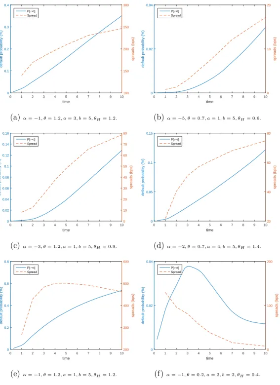
0 1 2 3 4 5 6 7 8 9 10 time 0 0.1 0.2 0.3 0.4 default probability (%) 100 150 200 250 300 spreads (bps) P[τ<t] Spread (a) α=−1, θ= 1.2, a= 3, b= 5, θH= 1.2. 0 1 2 3 4 5 6 7 8 9 10 time 0 0.02 0.04 default probability (%) 0 10 20 spreads (bps) P[τ<t] Spread (b) α=−5, θ= 0.7, a= 1, b= 5, θH= 0.6. 0 1 2 3 4 5 6 7 8 9 10 time 0 0.02 0.04 0.06 0.08 0.1 0.12 0.14 0.16 default probability (%) 0 10 20 30 40 50 60 70 80 spreads (bps) P[τ<t] Spread (c)α=−3, θ= 1.2, a= 1, b= 5, θH= 0.9. 0 1 2 3 4 5 6 7 8 9 10 time 0 0.05 0.1 0.15 default probability (%) 20 40 60 80 spreads (bps) P[τ<t] Spread (d) α=−2, θ= 0.7, a= 4, b= 5, θH= 1.4. 0 1 2 3 4 5 6 7 8 9 10 time 0 0.2 0.4 0.6 0.8 default probability (%) 200 300 400 500 600 spreads (bps) P[τ<t] Spread (e)α=−1, θ= 1.2, a= 1, b= 5, θH= 1.2. 0 1 2 3 4 5 6 7 8 9 10 time 0 0.02 0.04 default probability (%) 0 100 200 spreads (bps) P[τ<t] Spread (f)α=−1, θ= 0.2, a= 2, b= 2, θH= 0.4.
Figure 4: Term Structure of Default Probabilities and Spreads
Note: The graphs above are generated under Gamma specification both the idiosyncratic and common factor. The parameters that varies have their values specified under each graph while the rest of the parameters are kept constant (β= 0.7, aH = 2, bH = 3, H0=G0= ΣG0 = ΣH0 = 0.02, R= 0.4). The default
probabilities are computed for every quarter maturity starting withT = 0.25 until T = 10 while the spreads are computed for T = 1,3,5,7,10.The variety of
Standard practice assumes that default occurs half-way between coupon payments, see OKane and Turnbull (2003). Approximating (5.1), (5.2) and (5.3) by discretisation of the time line at the coupon payment nodestcgives:
VtP rot,dirty ≈ (1−R¯)X tc>t Bt max(tc−1, t) 2 EHtc[P ∗(τ ∈(max(t c−1, t), tc])] Accrtdef ≈ X tc>t Bt max(tc−1, t) 2 C[tc−max(tc−1, t)] 2∗360 EHtc[P ∗(τ ∈(max(t c−1, t), tc])] VtP rem,dirty ≈ CX tc> Bt(tc) tc−tc−1 360 EHtc[P ∗(τ > t c)] where P∗(τ > tc) = 1− p∗(tc) and P∗(τ ∈ (tc−1, tc]) = p∗(tc)− p∗(tc−1)
that can be easily computed by the formulae introduced in Section 4. The notation EHtc[.] shows calculation based on the density of the factor Htc.
In Figure 4 we present the resulting default probability curve and the associated spreads term structure for various sets of parameters. The model can generate various curve shapes, from the normal CDS curve (graphs 4a, 4b, 4c, 4d) in which the spreads increase with the time to maturity to inverted CDS curves (graph 4f) characterised by lower spreads for higher maturities.
5.2. Credit Default Swaps Index
If we denote byHt =PKj=1nj1{τi>t} the unit notional at timet, bynj the
percentage exposure10 to the namej, byR
j the respective recovery rate and by Bt(s) the discount factor, then the discounted cash-flows corresponding
10Usually computed as 1/K. For iTraxx n
to Protection Leg payments can be written as: WtP rot,dirty = E K X j=1 njBt(τj)(1−Rj)1{τj≤T} Ft = E E K X j=1 njBt(τj)(1−Rj)1{τj≤T} HT Ft = E K X j=1 njBt(τj∗)(1−R¯j)p∗j(T) Ft (5.4)
Again there may be a possible accrued coupon at the time of default. De-noting by Cidx the fixed coupon we have :
Adeft = E K X j=1 njBt(τi)1{τj≤T} Cidx(τ −max(tc:tc≤τ)) 360 Ft = E K X j=1 njBt(τ∗)p∗j(T) Cidx(τ −max(tc:tc≤τ)) 360 Ft (5.5) The present value of the cash-flows corresponding to the Premium Leg is:
WtP rem,dirty = E X tc>t Bt(tc)Cidx K X j=1 nj1{τj>tc} Ft = E X tc>t Bt(tc)Cidx K X j=1 nj(1−p∗(tc)) Ft (5.6)
An initial correction corresponding to the accrued coupon up to the trade date is computed similar as for the CDS contract Ainit
t = Cidx(
t−max(tc:tc≤t))
360
which leads to the index swap priceCDSIt=W
P rot,clean
t −W
P rem,clean
t . With
the assumption that defaults occur half-way between coupon payments:
WtP rot,dirty ≈ X tc>t Bt max(tc−1, t) +tc 2 K X j=1 nj(1−R¯j)EHtc[P ∗(τ j ∈(max(tc−1, t), tc])]
Adeft ≈ X tc>t Bt max(tc−1, t) +tc 2 Cidx[tc−max(tc−1, t)] 2∗360 K X j=1 njEHtc[P ∗ (τj ∈(max(tc−1, t), tc])] WtP rem,dirty ≈ Cidx X tc>t Bt(tc)tc−tc−1 360 K X j=1 njEHtc[P ∗ (τj > tc)]
where P∗(τ > tc) = 1−p∗(tc) and P∗(τ ∈ (tc−1, tc]) = p∗(tc)−p∗(tc−1) are
computed as for the CDS pricing.
In Figure 5 we present an analysis of the parameter’s impact on the shape of the spread curve for the CDSI of iTraxx Europe index. We fix the univariate parameters and focus on the multivariate parameters with impact on the CDSI price. Similar to Eckner (2009) we used a common level
α (estimated in our example at -5.5) which we multiply by the weight ωc computed as the ratio of the average 5y spreads over the entire portfolio and the 5y spread of the company (αc =−5.5ωc). The weight ωc represents the relative riskiness of the company when compared with the rest of the names in the index. The parameter β controls the dependence between the default probabilities for the obligors in the index. An increase inβ produces a rise in the spreads for the CDSI contract (see Figure 5a). This effect is usually more pronounced at longer maturities since for longer maturities there is time for the common factor to jump and create multiple defaults.
1 2 3 4 5 6 7 8 9 10 0 50 100 150 I II III (a)βI = 0.9, βII = 1.4, βIII = 0.6 1 2 3 4 5 6 7 8 9 10 0 20 40 60 80 100 120 140 160 I II III (b)θIH = 1.2, θHII = 1.6, θHIII = 0.6 1 2 3 4 5 6 7 8 9 10 0 50 100 150 200 250 300 I II III (c) aI H = 3, aIIH = 6, aIIIH = 1 1 2 3 4 5 6 7 8 9 10 0 50 100 150 200 250 I II III (d)bI H = 2, bIIH = 5, bIIIH = 1 1 2 3 4 5 6 7 8 9 10 0 50 100 150 I II III (e)αIr= 2, αIIr = 4, αIIIr = 1 1 2 3 4 5 6 7 8 9 10 0 50 100 150 200 250 I II III (f) βrI = 4, βrII = 6, βrIII = 2
Figure 5: Parameter Sensitivity of the CDSI Curve
Note: Term structure of CDSI spreads at the most important maturities for the iTraxx index with various parameter sets. The model used is IG-OU for both idiosyncratic and common factor. The initial parametersαc=−5.5ωc, θ= 1.2,
a= 2, b= 3, β =βs= 0.9, θH = 1.2, aH = 3, bH = 2, αr = 2, βr = 4,
H0 =G0= ΣG0 = ΣH0 = 0.02 are kept constant in all the graphs (model I) while
on e of the parameters that affect the entire index are changed one at a time 32
An opposite effect is observed in Figure 5b for the parameter θH. This parameter controls the speed of the mean reversion of the common factor. One expects that for higher values of θH the variance of the common factor will reverse faster to the long-run mean value, reducing the impact of the jumps in the common factor on the probability of default of the names in the portfolio. The same conclusion can be drawn for the parameter aH which controls the shape of the increments of the BDLP driving the variance of the common factor. Lower values of this parameter lead to a distribution of increments which is peaked closer to the origin implying smaller jump sizes of the common factor, and consequently a smaller importance of the common factor. This effect explains the lower spreads observed in Figure 5c. On the contrary, the effect of an increase in bH, the scale parameter of the distribution of common factor’s jumps, is to increase the level of spreads of the CDSI contract, as illustrated in Figure 5d. An explanation is that increasing bH implies a distribution for jumps of the common factor centred at higher values, creating more possibilities of default in the index portfolio. The last two analysed parameters control the distribution of the recovery rate. Here we used a discretization of a Beta(αr, βr) distribution to model the random recovery rate, assumed to be the same for all the names in the portfolio. Since the mean of a Beta distribution is αr
αr+βr the expected
recovery rate is positively related toαr and negatively related toβr. There is a negative linkage between the spreads of a CDSI contract and the expected recovery rate ¯R so an increase in αr leads to lower spreads, as in Figure 5e, while an increase in βr implies higher spreads as in Figure 5f. Similar observations can be made in the case of the IG-OU specification.
5.3. CDO tranches
A CDSI tranche is an option contract on the index, with the attachment
Al and detachment points Bl of a tranche l representing the interval of the cumulative loss process{Lt}t≥0to which the investors in that specific tranche
are exposed. For pricing CDO tranches we consider the cumulative loss
Ls =
PK
j=1nj(1−Rj)1{τj≤s}. Then the notional of a tranchel can be written
as Nstr(l) =fl(Ls) = (Bl−Al)−(Ls−Al)1{Ls>Al}+ (Ls−Bl)1{Ls>Bl}. The Premium Leg is T rP rem,dirtyt,l =E X tc>t Bt(tc)Ctrl Nttrc(l) Ft =X tc>t Bt(tc)Ctrl E[Nttrc(l)|Ft] (5.7)
and applying the market correction Ainit,lt = Cl tr
(t−max(tc:tc≤t))
360 leads to the
clean Premium price T rP rem,cleant,l = T rt,lP rem,dirty − Ainit,lt . With defaults halfway between coupon payments, the value of the Protection Leg and the accrued coupon at the time of default are:
T rP rot,dirtyt,l ≈ X tc>t Bt max(tc−1, t) +tc 2 E[Nttrc(l)−N tr(l) max(tc−1t)] Adeft ≈ X tc>t Bt max(tc−1, t) +tc 2 Ctrl [tc−max(tc−1, t)] 2∗360 E[N tr(l) tc −N tr(l) max(tc−1,t)]
The applicability of the formulae above depend on computing the val-ues E[Nttrc(l) − Nttrc−(1l)] = E[Nttrc(l)] −E[Nttrc−(l1)] and E[Nttrc(l)]. Since Nstr(l) =
fl(Ls) is a function of Ls for which we showed in Section 3.3 how to obtain its distribution, the computation of E[Nttrc(l)] is determined by the integral R
6. Calibration Methodology
The calibration of the model will use the information encoded in the term structure of CDS, CDSI and CDO tranches spreads. This requires the computation of the conditional probabilities of default, the conditional distribution of portfolio losses and the factor density for all the payment dates of the coupons11. For reducing the computational burden we follow Eckner
(2009) and Mortensen (2006) and compute the above value for intervals of one year length and use a cubic spline to interpolate for values at coupon dates in-between.
6.1. Univariate Calibration
The calibration of the default probability model for a specific name is based on CDS spreads or defaultable bond prices available on the market. The input observations can be either the market CDS rates or the implied probabilities of default bootstrapped from these spreads, see OKane and Turnbull (2003) for the bootstrapping procedure. In order to find the set of parameters Γc one could minimise the average relative percentage error:
ARP E = 1 M M X n=1 |Smarketn −Smodeln (Γ)| Sn market (6.1) whereM is the number of available market spreads/upfronts. Other measures of goodness-of-fit that are routinely used, see Schoutens et al. (2004), include RRMSE, APE and RMSE.
11For a 10 year maturity there are 40 payment dates for which these calculations need
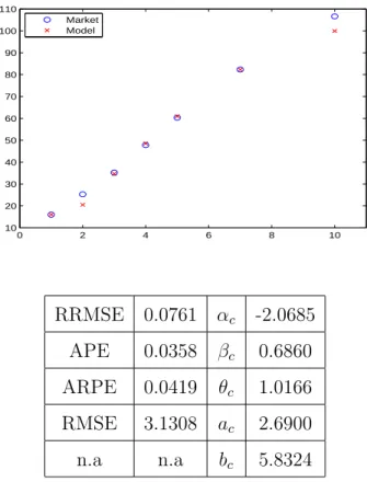
The example described here is for LafargeHolcim Ltd on the date 18 Feb 2015, with CDS market prices downloaded from Bloomberg. For the interest rate we used the swap curve data available in Bloomberg which consists of Euribor rates for maturities under one year and rates striped form interest rate swap prices for longer maturities.
0 2 4 6 8 10 10 20 30 40 50 60 70 80 90 100 110 Market Model RRMSE 0.0761 αc -2.0685 APE 0.0358 βc 0.6860 ARPE 0.0419 θc 1.0166 RMSE 3.1308 ac 2.6900 n.a n.a bc 5.8324
Figure 6: Calibration of LafargeHolcim Ltd CDS term structure
Note: The Gamma-OU model is calibrated on LafargeHolcim Ltd CDS term structure data available in Bloomberg for the date 18 Feb. 2015. The parameters of the common factor are fixed (θH = 0.6, aH = 2, bH = 3,R¯ = 0.4) while the free parameters parameters free (αc, βc, θc, ac, bc) are implied from the calibration with the goodness-of-fit measured by RRMSE, APE, ARPE and RMSE.
Since we are interested in the performance of the univariate default prob-ability model, we fix the parameters of the common factor to θH = 0.6, aH = 2, bH = 3,R¯ = 0.4 wile letting the other parameters free (αc, βc, θc, ac, bc). The results of the univariate calibration presented in Figure 6 indicate that the model fits well the data.
6.2. Multivariate Calibration
The multivariate calibration of the model requires the joint calibration of CDS , CDSI and index tranches spreads. The market data used for cali-bration purpose regards the trading date 18 Feb. 2015 and was downloaded from Bloomberg. It corresponds to the CDS spreads for maturities (3y, 5y, 7y, 10y) for each of the 125 components of the iTraxx Series 22 index, the CDSI prices on the iTraxx Series 22 index for maturities (3y, 5y, 7y, 10y) and the spreads for the 0−3%, 3−6%, 6−12% and 12−100% tranches on the index for maturities (3y, 5y).12 The total error to minimise is the (weighted) sum of the errors on CDS spreads, CDSI spreads and tranches spreads:
min
Γ
ARP ECDS(Γ) + 5ARP ECDSI(Γ) + 5ARP Etr(Γ) (6.2)
where ARP ECDS(Γ) = 1 N 1 M N X n=1 M X m=1 |Smarket,CDSn,m −Smodel,CDSn,m (Γ)| Smarket,CDSn,m (6.3) ARP ECDSI(Γ) = 1 M M X m=1 |Sm market,CDSI−Smodel,CDSIm (Γ)| Sn market,CDSI (6.4)
12Some of the tranches are quoted in upfront points and have been transformed to
ARP Etr(Γ) = 1 P 1 M P X p=1 M X m=1 |Smarket,trm,p −Smodel,trm,p (Γ)| Smarket,trm,p (6.5)
for n = 1,2,3, ..., N = 125 names in the index portfolio, m = 1,2, ..., M
maturities and p= 1,2, ..., P tranches available.
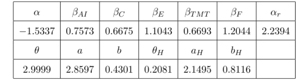
Table 1: Parameters from the multivariate calibration
Note: The parameters resulted from the calibration of the multivariate model on the 22nd series of the iTraxx index CDSI term structure data available in
Bloomberg for the date 18 Feb. 2015. The model used for the factors is Gamma-OU.
α βAI βC βE βT M T βF αr
−1.5337 0.7573 0.6675 1.1043 0.6693 1.2044 2.2394
θ a b θH aH bH
2.9999 2.8597 0.4301 0.2081 2.1495 0.8116
The general model employed here has (N ×5) + 5 parameters, five uni-variate parameters corresponding to each obligor in the credit portfolio ofN
names and five common parameters. For the purposes of having a more par-simonious model we adopt a series of simplifying assumptions. The first as-sumption is that the individual barrier levelαccan be expressed as αc=αωc for a general levelα and a weight ωc=
CDS5c
avgCDS5 obtained as the quotient
be-tween the 5y CDS level of individual names and the average 5y CDS for the entire portfolio of credit names. The second assumption is that each obligor in a specific sector responds in the same way to the shocks from the market factor.
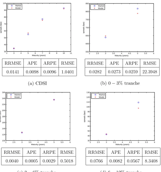
2 3 4 5 6 7 8 9 10 11 30 40 50 60 70 80 90 100 Maturity (years) spreads (bps) Market Model
RRMSE APE ARPE RMSE
0.0141 0.0098 0.0096 1.0401 (a) CDSI 2 2.5 3 3.5 4 4.5 5 5.5 6 550 600 650 700 750 800 850 Maturity (years) spreads (bps) Market Model
RRMSE APE ARPE RMSE
0.0282 0.0273 0.0259 22.3948 (b) 0−3% tranche 2 2.5 3 3.5 4 4.5 5 5.5 6 100 120 140 160 180 200 220 240 260 Maturity (years) spreads (bps) Market Model
RRMSE APE ARPE RMSE
0.0040 0.0005 0.0029 0.5018 (c) 3−6% tranche 2 2.5 3 3.5 4 4.5 5 5.5 6 30 40 50 60 70 80 90 100 110 120 130 Maturity (years) spreads (bps) Market Model
RRMSE APE ARPE RMSE
0.0766 0.0082 0.0567 8.3408
(d) 6−12% tranche
Figure 7: Multivariate Calibration Results
Note: The multivariate model is calibrated on CDSI and index tranches data on iTraxx index available from Bloomberg for the date 18 Feb. 2015. The model used for the factors is Gamma-OU. The parameters the calibration are presented in Table 1. Four measures of goodness of fit (RRMSE, APE, ARPE and RMSE) are also displayed in the tables bellow each graph.
As a result we reduced the number of βc parameters from N = 125 to only 5 beta values βAI, βC, βE, ββAI, βF corresponding to the five sectors
di-vision of the names in the iTraxx index (Autos & Industrials, Consumers, Energy, Technology & Media & Telecommunications and Financials). The last assumption is that the parameters θ, aand b which control the distribu-tion of the company specific factor are common to all the companies in the index. The results of the multivariate calibration are presented in Table 1. As can be seen from the measure of goodness of fit presented in the table, the multivariate model fits well the market data.
7. Conclusions
In this paper we developed a factor structure of the time-changes driving the impact of the information arrival on the credit worthiness process. More-over we proposed a new FFT based general methodology for the computa-tion of the probability of default which allows the extension of the univariate model to specifications not possible under the Panjer recursion technology used in recent credit risk literature.
Under our framework it is feasible to price single-name CDS, CDSI and index tranches contracts or CDOs. A useful and interesting characteristic of our proposed multivariate model, that stems from the use of mean reverting models for the variance of the common factor, is the ability of producing “contagion-like” effects observed in the market.
This paper described the set-up of the credit modelling framework based on Brownian time-changed processes with volatility belonging to the class of mean reverting L´evy driven OU type process. Within this framework flexible
formulae were derived for CDS prices, credit index prices and CDO/tranche prices. The next challenge would be to link the drivers of this models to sectoral and macroeconomic effects such as described by Chava et al. (2011).
Appendix A. Proof Proposition 2
Because Υ has a chi-squared distribution with one degree of freedom so
Υ ∼Γ(1/2,2) andk−2Υ ∼Γ(1/2,2a−2). Then 1
k−2Υ has an inverted Gamma
(or inverted chi-squared) distribution with density:
f(1/x) = k
n
2n/2Γ(n/2)x
(n+2)/2e−xk2
2 (A.1)
and the characteristic function as given in Witkovsk`y (2001),with n = 1 in our case, where Γ(x) is the Gamma function andKα(x) is the Bessel function of the second kind:
φiΓ(u) =
2(−2iuk−2)n/4K
n/2[k2(−2iuk−2)1/2]
(2k−2)n/2Γ(n/2) (A.2)
Taking the square of a standard normal variable byΥ =Z2 and denoting
υ = γ−ck2 for constants k <0, γ >0, c > given that γ−c >0, we can write:
P Υ ≤υ = P Z2 ≤ k 2 γ−c =P |y| ≤√z = P Z ≤ √|k| γ−c − 1−P Z ≤ √|k| γ−c = 2P Z ≤ √|k| γ−c −1 (A.3)
Standard probability calculus gives P Z ≤ √−k γ−c = 1−P Z ≤ √k γ−c so 2P Z ≤ √a γ−c = 1−P Υ ≤ k2 γ−c =P 1 k−2Υ ≤γ−c .
Therefore we can write the default probability (3.1) as P(τ < s|Ft) = E[2P(Z p Γs−Γt−(b−Xt)≤0|Γs)|Ft] = E 2P Z ≤ √(b−Xt) Γs−Γt Γs Ft = E P 1 (b−Xt)−2Υ ≤(Γs−Γt) Γs Ft = E P 1 (b−Xt)−2Υ −(Γs−Γt)≤0 Γs Ft (A.4) The variable inside (A.4) is the difference of two independent variables: the first is an inverted Gamma with characteristic function given by (A.2) and the second is just the distribution of the integrated variance for which the characteristic function of various specifications will be discussed in Section 4. Now the conditional probability of default given the factor Hs is:
P(τ < s|Hs∨ Ft) = E P 1 (b−Xt)−2Υ −(Gs−Gt)−β(Hs−Ht)≤0 Hs∨ Ft = E[P(Q≤0)|Hs∨ Ft] (A.5) where Q= (b−X1 t)−2Υ −(Gs−Gt)−β(Hs−Ht).
Appendix B. Proof Proposition 3
The formulae follow by just writing the characteristic function of Q =
1
(b−Xt)−2Υ −(Gs−Gt)−β(Hs−Ht) as function of the characteristic functions
of the inverse Gaussian variable (b−X1
t)−2Υ and of the variables Gs and Hs :
PGill[τ < s|Hs∨ Ft] = 1 2− 1 π Z ∞ 0 < φ Q|H(u) iu du = 1 2− 1 π< Z ∞ 0 e−iu(βHs)φiΓ(u)φGs(−u)e iu(βHt+Gt) iu du (B.1)
PKim[τ < s|Hs∨ Ft] = 1 π Z ∞ 0 < φQ|H(u+iρ) ρ−iu du = 1 π< Z ∞ 0
e−iu(βHs)φiΓ(u+iρ)φGs(−u−iρ)e
iu(Gt+βHt)+ρ(β(Ht−Hs)+Gt) ρ−iu du (B.2) PHilb[τ < s|Hs∨ Ft] = 1 2− i 2H[φQ(0)](0) = 1 2 − i 2H[φiΓ(u)φGs(−u)e −iu(Gt+βHt−βHs)](0) ≈ 1 2 − i 2 M X m=−M,m6=0 φiΓ(mh)φGs(−mh)e imh(Gt+βHt−βHs)1−cos(−πm) −πm = 1 2− i 2 M X m=−M,m6=0 φiΓ(mh)φGs(−mh)e imh(Gt+βHt−βHs)1−(−1) −m −πm = 1 2− i 2 M−1 X m=0 e−2imh(βHs)2φiΓ((2m+ 1−M)h)φGs((M −2m−1)h)e ihΛ π(M −2m−1) (B.3) where we used the notation Λ = (2m+ 1−M)((Gt+βHt)−βHs(1−M)).
References
Andersen, L., Sidenius, J., 2004. Extensions to the gaussian copula: Random recovery and random factor loadings. Journal of Credit Risk Volume 1, 27–70.
Andersen, L., Sidenius, J., Basu, S., 2003. All your hedges in one basket. RISK 16, 67–72.
Ballestra, L.V., Pacelli, G., 2014. Valuing risky debt: A new model com-bining structural information with the reduced-form approach. Insurance: Mathematics and Economics 55, 261–271.
Barndorff-Nielsen, O., Shiryaev, A., 2010. Change of time and change of measure. volume 13. World Scientific.
Barndorff-Nielsen, O.E., 2001. Superposition of Ornstein–Uhlenbeck type processes. Theory of Probability & Its Applications 45, 175–194.
Barndorff-Nielsen, O.E., Shephard, N., 2001. Non-gaussian ornstein– uhlenbeck-based models and some of their uses in financial economics. Journal of the Royal Statistical Society: Series B (Statistical Methodol-ogy) 63, 167–241.
Baxter, M., 2007. Gamma process dynamic modelling of credit. Risk 20, 98–101.
Bielecki, T.R., Cr´epey, S., Jeanblanc, M., 2010. Up and down credit risk. Quantitative Finance 10, 1137–1151.
Blanchet-Scalliet, C., Patras, F., Bielecki, T.R., Brigo, D., Patras, F., 2011. Structural counterparty risk valuation for credit default swaps. Credit Risk Frontiers: Subprime Crisis, Pricing and Hedging, CVA, MBS, Ratings, and Liquidity , 437–455.
Cariboni, J., Schoutens, W., 2007. Pricing credit default swaps under L´evy models. Journal of Computational Finance 10, 71–91.
Cariboni, J., Schoutens, W., 2009. Jumps in intensity models: investigating the performance of Ornstein-Uhlenbeck processes in credit risk modeling. Metrika 69, 173–198.
Chava, S., Stefanescu, C., Turnbull, S., 2011. Modeling the loss distribution. Management Science 57, 1267–1287.
Cont, R., Minca, A., 2013. Recovering portfolio default intensities implied by CDO quotes. Mathematical Finance 23, 94–121.
Cont, R., Savescu, I., 2008. Frontiers in Quantitative Finance: Credit Risk and Volatility Modeling. Wiley, New York. chapter Forward equations for portfolio credit derivatives. p. 269288.
Dai, Q., Singleton, K., 2003. Term structure dynamics in theory and reality. Review of Financial Studies 16, 631–678.
Davis, M., Lo, V., 2001. Infectious defaults. Quantitative Finance 1, 382–387. Eckner, A., 2009. Computational techniques for basic affine models of
port-folio credit risk. Journal of Computational Finance 13, 63–97.
Epstein, C.L., Schotland, J., 2008. The bad truth about Laplace’s transform. SIAM review 50, 504–520.
Feng, L., Lin, X., 2013. Inverting analytic characteristic functions and finan-cial applications. SIAM Journal on Finanfinan-cial Mathematics 4, 372–398. Gatarek, D., Jab lecki, J., 2013. A model for dependent defaults and pricing
contingent claims with counterparty risk. Technical Report. National Bank of Poland, Economic Institute.
Hao, X., Li, X., 2015. Pricing credit default swaps with a random recovery rate by a double inverse Fourier transform. Insurance: Mathematics and Economics 65, 103–110.
Hao, X., Li, X., Shimizu, Y., 2013. Finite-time survival probability and credit default swaps pricing under geometric L´evy markets. Insurance: Mathematics and Economics 53, 14–23.
Hull, J.C., White, A.D., 2004. Valuation of a CDO and an n-th to default CDS without Monte Carlo simulation. The Journal of Derivatives 12, 8–23. Hurd, T., Zhou, Z., 2011. Structural credit risk using time-changed brownian motions: a tale of two models. Working paper. Department of Mathematics and Statistics, McMaster University .
Hurd, T.R., 2009. Credit risk modeling using time-changed Brownian motion. International Journal of Theoretical and Applied Finance 12, 1213–1230. Kijima, M., Siu, C.C., 2014. Credit-equity modeling under a latent L´evy
firm process. International Journal of Theoretical and Applied Finance 17, 1–41.
Kim, Y.S., Rachev, S., Bianchi, M.L., Fabozzi, F.J., 2010. Computing VaR and AVaR in infinitely divisible distributions. Probability and Mathemat-ical Statistics 30, 223–245.
MacKenzie, D., Spears, T., 2014. The formula that killed wall street? the gaussian copula and modelling practices in investment banking. Social Studies of Science 44, 393–417.
MARKIT, 2009. The CDS Big Bang: Understanding the Changes to the Global CDS Contract and North Amerian Conventions. Technical Report. Mortensen, A., 2006. Semi-analytical valuation of basket credit derivatives
in intensity-based models. The Journal of Derivatives 13, 8–26.
Nicolato, E., Venardos, E., 2003. Option pricing in stochastic volatility mod-els of the Ornstein-Uhlenbeck type. Mathematical finance 13, 445–466. Norberg, R., 2004. Vasiˇcek beyond the normal. Mathematical Finance 14,
585–604.
OKane, D., Turnbull, S., 2003. Valuation of credit default swaps. Lehman Brothers Quantitative Credit Research Quarterly 2003, Q1–Q2.
Packham, N., Schloegl, L., Schmidt, W.M., 2013. Credit gap risk in a first passage time model with jumps. Quantitative Finance 13, 1871–1889. Schneider, P., S¨ogner, L., Veza, T., 2010. The economic role of jumps and
recovery rates in the market for corporate default risk. Journal of Financial and Quantitative Analysis 45, 1517–1547.
Schoutens, W., Simons, E., Tistaert, J., 2004. A perfect calibration! now what? Wilmott Magazine .
Tauchen, G., Zhou, H., 2011. Realized jumps on financial markets and pre-dicting credit spreads. Journal of Econometrics 160, 102–118.
Wei, L., Yuan, Z., 2016. The loss given default of a low-default portfolio with weak contagion. Insurance: Mathematics and Economics 66, 113–123.
Witkovsk`y, V., 2001. Computing the distribution of a linear combination of inverted gamma variables. Kybernetika 37, 79–90.
Zhang, B., Zhou, H., Zhu, H., 2009. Explaining credit default swap spreads with the equity volatility and jump risks of individual firms. Review of Financial Studies 22, 5099–5131.