An MVAR Framework to Capture Extreme Events in Macroprudential Stress Tests

CAHIER D’ÉTUDES

WORKING PAPER

N° 63

AN MVAR FRAMEWORK TO CAPTURE EXTREME EVENTS

IN MACRO-PRUDENTIAL STRESS TESTS

Paolo GUARDA, Abdelaziz ROUABAH and John THEAL

Contents

Introduction ... 4

2. The SUR model: Contemporaneous correlation in the innovations ... 7

3. The MVAR Model: A tool to capture extreme events ... 9

4. The Variable Neighbourhood search... 12

5. Data and estimation of the SUR Model ... 14

6. Implementation of EMVNS and the estimation of the MVAR model... 15

7. The Kullback-Leibler measure of divergence... 20

8. Conclusion... 22

An MVAR Framework to Capture Extreme Events in

Macro-prudential Stress Tests

♣

Paolo Guarda1_{, Abdelaziz Rouabah}2 _{and John Theal}3

Abstract

The stress testing literature abounds with reduced-form macroeconomic models that are used to forecast the evolution of the macroeconomic environment in the context of a stress testing exercise. These models permit supervisors to estimate counterparty risk under both baseline and adverse scenarios. However, the large majority of these models are founded on the assumption of normality of the innovation series. While this assumption renders the model tractable, it fails to capture the observed frequency of distant tail events that represent the hallmark of systemic financial stress. Consequently, these kinds of macro models tend to underestimate the actual level of credit risk. This also leads to an inaccurate assessment of the degree of systemic risk inherent in the financial sector. Clearly this may have significant implications for macro-prudential policy makers. One possible way to overcome such a limitation is to introduce a mixture of distributions model in order to better capture the potential for extreme events.

Based on the methodology developed by Fong, Li, Yau and Wong (2007), we have incorporated a macroeconomic model based on a mixture vector autoregression (MVAR) into the stress testing framework of Rouabah and Theal (2010) that is used at the Banque centrale du Luxembourg. This allows the counterparty credit risk model to better capture extreme tail events in comparison to models based on assuming normality of the distributions underlying the macro models. We believe this approach facilitates a more accurate assessment of credit risk.

JEL classification: C15, E44, G01, G21

Keywords: financial stability, stress testing, MVAR, mixture of normals, VAR, tier 1 capital ratio, counterparty risk, Luxembourg banking sector

♣_{The authors of this paper are grateful to C. S. Wong and T. P. Fong for their valuable help}

and suggestions and for their explanation of the calculation of the standard errors for the estimated MVAR parameters. The opinions and empirical analyses provided in this paper are those of the authors and do not necessarily reflect the views or opinions of the Banque centrale du Luxembourg.

1_{Banque centrale du Luxembourg. Email address: Paolo.Guarda@bcl.lu}

2 _{Banque centrale du Luxembourg. Email address: Abdelaziz.Rouabah@bcl.lu} 3 _{Banque centrale du Luxembourg. Email address: John.Theal@bcl.lu}

Résumé non-technique

La conduite des stress-tests constitue un levier principal parmi les outils d’évaluation de la solidité des composantes du système financier. Ils représentent, par ailleurs, un instrument important pour les banques centrales dans le cadre de leur surveillance macro-prudentielle. Cependant, une multitude de méthodologies coexistent pour quantifier l’impact de la survenance des chocs sévères, mais plausibles, sur la solidité financière de l’une des composantes du système financier.

Le point commun à l’ensemble des travaux dédiés aux tests de résistance macro-prudentiels est leur appui sur des modèles de formes réduites, estimés et/ou simulés en adoptant l’hypothèse de normalité de la distribution des innovations (chocs). Or, ce type de postulat est susceptible de minimiser l’importance des risques extrêmes ou d’ignorer l’existence de la bi-modalité de la distribution des phénomènes étudiés. Autrement dit, ce type de biais est synonyme d’une minimisation des risques auxquels le système financier serait confronté. De plus, ce biais serait également un facteur de minimisation des risques dans la prise de décision en matière de politique macro-prudentielle pour contenir la matérialisation d’évènements sévères.

Soucieux des limites des approches traditionnelles, les auteurs de cette étude ont conçu un modèle spécifique pour la conduite des stress-tests pour le secteur bancaire luxembourgeois en s’appuyant sur une nouvelle méthodologie d’estimation développée par Fong et al. (2007). Il s’agit d’une spécification MVAR avec une mixture de deux distributions (Mixture Vector Autoregressive Model) permettant ainsi de capturer de manière plus précise l’importance du risque de crédit propre au secteur bancaire. Dans ce cadre, le risque de crédit a été approximé par une transformation logistique du ratio des provisions par rapport à l’encours des crédits attribués à la clientèle y compris interbancaire.

La comparaison des résultats issus du Modèle MVAR et ceux du Modèle de régressions apparemment indépendantes (SUR) laisse présager l’existence d’un biais important, spécifique à ce dernier et qui s’explique par la normalité des distributions sous-jacentes aux méthodes économétriques standards. En réalité, les résultats de nos estimations du modèle SUR révèlent une sous-estimation significative du risque du crédit dû aux contreparties des banques luxembourgeoises. En d’autres termes, le modèle SUR indique que la probabilité de défaut des contreparties serait moins élevée en comparaison avec celles issues du Modèle MVAR. En effet, la mixture de distributions dans le modèle MVAR issue de notre processus d’optimisation est bimodale. Ainsi, contrairement à la distribution symétrique qui caractérise le modèle SUR, celle du Modèle MVAR semble attribuer une pondération plus importante aux variations négatives de l’indicateur du risque de crédit.

1. Introduction

From a macro-prudential perspective, the efficacy of a top-down stress testing program is strongly influenced by the degree to which the stress test methodology transmits and captures the effects of the stressed macro factors on banks’ balance sheets. This helps to provide insight into the linkages between the financial system and the real economy. Following the recent financial crisis, national supervisory authorities significantly amended their macro-prudential surveillance frameworks so that they would be better equipped to detect, and therefore mitigate, the build-up of systemic risk. At the European level, the recently established European Banking Authority (EBA) has undertaken a concerted and annual effort to stress test the EU-wide banking sector. This large-scale exercise is intended to assess the solvability and funding conditions of Europe’s largest and most systemically relevant financial institutions. The stress test conducted by the EBA is a constrained bottom-up exercise, designed to assess the financial soundness of institutions at an individual level. This kind of exercise is therefore “bottom-up” in its design although not necessarily in its execution. However, despite these efforts, as Borio (2010) notes, regulators must assess the financial sector using a system-wide approach as a complement to supervision at the individual institutional level. Only in this context can authorities take into account the endogenous factors that influence financial stability and tend to create the potential for systemic disruption of the financial intermediation process. Borio (2009) notes that if one lesson has been learned in the post-crisis period it is that although financial institutions may appear to be financially sound under a purely micro-prudential assessment, there may be latent factors negatively affecting the system at the macro-prudential level and resulting in an accumulation of systemic risk.

In order to address these “hidden” or latent systemic risks, the micro-prudential approach4

must be accompanied by a macro-prudential surveillance program. In the effort to improve risk management practice, a trend towards “top-down” stress testing has emerged in the post-crisis period. In Europe, both national authorities and the ECB with potential future input to the newly established European Systemic Risk Board (ESRB) have demonstrated their initiative for conducting top-down analyses of the solvability of both their respective national and EU-wide financial sectors. This top-down approach is an important complement to the micro-prudential perspective. Indeed, Borio (2009) suggests that the micro-prudential approach to supervision can be compared to the management of a portfolio of securities in which there is an equivalency between a security and a financial institution. Conversely, in the macro-prudential case it is the correlation between common exposures in the banking sector that needs to be monitored as these can give rise to systemic risk that may affect the entire sector rather than a single institution. From a micro-prudential perspective, such sources of risk are considered latent. For this reason, it is imperative that

national authorities evaluate not only individual financial institutions for risk, but also their entire banking and financial sectors. This is the role of the top-down stress test.

Currently, there is no single or canonical methodology for conducting a top-down test, although variations on the framework originally used by Wilson (1997a, 1997b) seem to be quite commonly employed. In any case, this lack of consensus has resulted in a diverse array of stress testing methodologies proposed in the academic literature. Sorge (2004) provides a comprehensive review of some common methodologies that have been used in the recent past. Nevertheless, a few specific models warrant being mentioned. Virolainen (2004) used data on corporate sector bankruptcies in order to estimate a macro-economic model for the Finnish corporate sector. Using this methodology Virolainen was able to link default rates in the corporate sector to selected macroeconomic variables that include GDP, interest rates and the level of indebtedness. The estimated equations are then used to assess the impact of adverse macroeconomic events on bank’s corporate credit portfolios. In Virolainen’s case, the model consists of univariate autoregressive equations with a maximum lag of two quarters. These equations rely on the assumption of normality in the

innovation series5. Under such an assumption Virolainen then simulates loss distributions of

Finnish corporate sector portfolios under various macroeconomic shocks. However, he encounters some difficulties incorporating the interest rate into the model

Huang et al. (2009) proposed a method for stress testing a group of financial institutions using risk-neutral probabilities of default (PD) and an integrated micro-macro model that accounts for dynamic linkages between institutions and macro-financial conditions. This allowed them to calculate an insurance premium that could be charged in order to protect such institutions against a specified level of loss. This is convenient for supervisory authorities as it provides a quantitative assessment that could be integrated into a rules-based macro-prudential surveillance framework. However, their stress-testing scenarios are based on the results of a VAR model. The VAR framework also assumes normality of the innovation series and this can affect the magnitude of the probability of default emanating from the model. In this case, there is a risk that the significance of the actual level of risk may be underestimated.

Wong et al. (2006) have developed a framework for stress testing Hong Kong’s retail banks that incorporates macroeconomic credit risk models in order to provide the linkage between such macroeconomic variables as GDP and property prices to banks’ loan portfolios. Using their estimated macro model to perform Monte Carlo simulations, the authors are able to introduce adverse macroeconomic shocks in order to study their effect on credit portfolios. This allows them to construct a probability distribution of credit losses that can then be used to calculate value at risk (VaR) statistics. This method is quite general and can be extended to portfolios other than mortgage exposures. Rouabah and Theal (2010) adapted the work

of Wong et al. (2006) to Luxembourg’s banking sector. Additionally, by extending the Monte Carlo simulations they were able to estimate Basel II tier 1 capital requirements for the banking sector of Luxembourg. They found that banking sector counterparties in Luxembourg remained particularly sensitive to changes in euro area real GDP growth as well as to housing market prices. The sensitivity to euro area GDP was attributed to the large number of foreign subsidiaries with operations in Luxembourg.

It should be noted that such credit risk assessment models are not solely limited to the banking and financial sector. Indeed, Yan et al. (2009) use a seemingly unrelated regression (SUR) model in combination with a copula-based simulation process to provide an assessment of farm credit risk. This allowed them to determine a farm’s ability to meet its financial obligations within a pre-specified time horizon. The SUR model itself is used to estimate a farm’s ratio of assets to expected debt. Provided the requisite data is available, this model could also be extended and applied to financial institutions.

In the context of their macroeconomic frameworks, the various models discussed above all assume that errors follow a univariate normal distribution. This allows estimation to proceed by OLS, SUR or VAR. However, some approaches in the literature consider multivariate

error distributions. For example, Boss et al. (2006) developed the Systemic Risk Monitor

(SRM), as a tool for financial stability analysis and off-site supervision of banking institutions. Methodologically, the SRM combines a credit risk analysis with a network analysis of the banking system in order to gauge the level of systemic risk. This provides an assessment of the likelihood of financial distress in addition to the potential losses that may be incurred in a systemic event. The design of the system is modular and it incorporates a macro model that links changes in macro variables to the risk factors of the model. The risk factor distribution is taken to be multivariate and is, in part, implemented using a grouped t-copula.

Mixed normal models seem to be attracting increased attention in the recent literature. Using Monte Carlo simulations, Maciejowska (2010) employs a mixed normal structural VAR, or SVAR, model as the basis for a comparison of maximization algorithms. Maciejowska finds that the EM algorithm outperforms other more general estimation methods such as Broyden-Fletcher-Goldfarb-Shanno (BFGS), Newton and Berndt-Hall-Hall-Hausman (BHHH) methods. In this paper, we estimate the MVAR model using a modified version of the EM algorithm.

Fong et al. (2008) have introduced a mixture vector autoregressive (MVAR) model into the stress testing literature. This allows the link between default rates and macro conditions to differ according to market conditions. In the context of a VAR framework, the model explicitly accommodates changes in financial fragility and allows them to feed back into the macroeconomic model. This MVAR framework provides a very flexible econometric structure that is also capable of capturing some of the tail risk that models based on a univariate normal distribution neglect. In the context of this new framework, the authors find that, compared to the more common unimodal models, credit losses in the face of adverse

shocks tend to double. This suggests that the more traditional VAR, SUR and OLS models may habitually underestimate potential credit losses.

In this paper, we use the MVAR framework derived by Fong et al. (2007) to extend the previous work of Rouabah and Theal (2010) to evaluate credit risk for Luxembourg’s banking sector. We propose an empirical measure of “bias” between the results based on a mixture of normals and those based on a univariate normal distribution. In a related application of this methodology, it would also be possible to use the model’s output to calculate the new Basel II tier 1 capital ratios under the MVAR framework and compare these to the values calculated using a SUR model.

This paper is structured as follows. First, we present a brief overview of the predecessor SUR framework employed in Rouabah and Theal (2010). In section 3 we present the MVAR model estimation procedure and empirical results. In the fourth section we provide a description of the Expectation Maximization Variable Neighbourhood Search (EMVNS) algorithm used to improve the EM estimates. Section 5 contains a description of the data and the results of the SUR estimation. The EMVNS estimation of the MVAR is detailed in section 6. In section 7 we propose an empirical measure of “divergence” between SUR results assuming univariate normal distributions and results based on MVAR models allowing for a mixture of distributions. Lastly we conclude.

2. The SUR model: Contemporaneous correlation in the innovations

The SUR model discussed in Rouabah and Theal (2010) consists of four equations that include a proxy for banks’ counterparty probability of default. Specifying the model in this manner allowed them to take into account the relation between the macroeconomic variables and banks’ counterparty risk. In order to estimate the probability of default of the Luxembourg banking sector’s counterparties, an aggregate balance sheet was constructed using the ratio of provisions on loans to total loans over all sectors. This ratio was then used as a proxy for the aggregate probability of default, thereby providing a metric for assessing the vulnerability of the Luxembourg financial system to various adverse macroeconomic scenarios. The adverse scenarios were implemented by applying a series of shocks during a Monte Carlo simulation procedure.

The historical probability of default series consisted of quarterly observations over the period

from the first quarter of 1995 until the third quarter of 2009. Since

p

_t is a probability, and

therefore lies in the fixed interval

[ ]

0,1 , a logit transform given by equation (1), was applied to

shift the probabilities into the set of real numbers. The analytical form of the logit transform is expressed in equation (1):

⎟⎟ ⎠ ⎞ ⎜⎜ ⎝ ⎛ ₋ = t t t p p y ln 1 (1)

This expression transforms

p

_t such that

y

_t takes on values in the interval

−

∞

<

y

_t

<

∞

.

Note that

y

_t and

p

_t are inversely related. The same will apply to their first differences.

Econometrically, the macroeconomic time series are required to be stationary so the first differences of the log of euro area and Luxembourg real GDP along with the first differences of the series for real property prices were employed throughout the estimation.

In detailed terms, the macroeconomic model consists of a joint system of six linear equations for the probability of default, the growth rate of Luxembourg GDP, the euro area real GDP growth rate, the real interest rate, the change in real property prices, and returns on the SX5E index. This specification allows for feedback effects from macroeconomic variables onto the probability of default series. Furthermore, using one or two lags of the endogenous variable in each equation allows for the persistence and transmission of exogenous shocks through the system. Through the SUR specification, the probability of default can be related to a group of macroeconomic variables thereby linking the fundamental economic environment to the vulnerability of the banking sector as a whole. Any correlation between shocks is captured by the variance covariance matrix of the residual series. This matrix is used to impose the characteristic correlation structure on the macroeconomic variables when conducting the Monte Carlo simulations.

The equations for the probability of default and the macroeconomic variables are given by equations (2) and (3), respectively:

t k t k t s t s t t

m

A

x

A

x

Φ

y

Φ

y

ν

y

=

+

1

+

K

+

1_{+ −}

+

1 ₋1

+

K

+

₋

+

(2) t p t p t t

n

B

x

B

x

ε

x

=

+

1 −1

+

K

+

−

+

(3)

In our case,

y

_t is

1

×

1

,

x

_t is an

M

×

1

vector of

M

macroeconomic variables,

A

_1+s is

M

×

1

, and

Φ

_k,

y

_t−k and

ν

_tare scalars. Finally,

B

_p is an

M

_×

M

coefficient matrix and

ε

_t

is an

M

×

1

vector of independent and identically normally distributed disturbances. The

variance covariance matrix,

E

, is given by:

( )

⎥ ⎦ ⎤ ⎢ ⎣ ⎡ = ⎟⎟ ⎠ ⎞ ⎜⎜ ⎝ ⎛ = ε ε ν, ε ν, ν Σ Σ Σ Σ Σ Σ 0 ε ν E ~ N , , (4)

This specification links the probability of default series to the evolution of the macroeconomic environment. Incorporating lagged values of the dependent variables allows for the persistence and transmission of exogenous shocks through the system. This approach is similar to a restricted VAR as opposed to the standard VAR models used in Hoggarth,

Sorensen and Zicchino (2004) and Filosa (2007). However both fail to sufficiently capture tail effects.

The estimation results showed that increases in the growth rate of both Luxembourg and

euro area GDP result in an increase in the value of the transformed variable

y

_t which is

inversely related to the probability of default. Correspondingly, a decrease in euro area or Luxembourg economic growth could result in a positive increase in this probability of default, thereby increasing the risk for the Luxembourg banking sector. A similar effect can be observed for the property price index, although there is a considerable amount of uncertainty surrounding the coefficient estimate. In addition, an increase in the real interest rate will

negatively affect

y

_t. Finally, the coefficient on the lagged probability of default was found to

be positive and significant which suggests that exogenous shocks will persist for a time horizon exceeding the duration of the shock. The same is true for the macroeconomic variable equations. The model seems to capture the expected dynamics between the macro-economy and the probability of default.

3. The MVAR model: A tool to capture extreme events

In order to improve its macro-prudential assessment framework, the Banque centrale du Luxembourg actively engages in regular research that is specifically intended to improve the ability of its stress testing exercise to detect and quantify the level of credit risk within the banking sector of Luxembourg. This section of the paper reports the initial results of a study that compares a new stress testing model developed by the BCL to the results of an earlier SUR-based model discussed above. This analysis makes it possible to evaluate any divergence between the two models suggesting possible under-estimation of bank credit risk.

The BCL’s new stress testing methodology incorporates the mixture vector autoregressive model (MVAR) in order to better capture the tail component of the distribution of credit risk in Luxembourg’s financial sector. As discussed in Fong et al. (2008), this can lead to a more accurate assessment of credit risk. Whereas the MVAR model uses a mixture of distributions to model credit risk, most stress-testing models assume a unimodal distribution of errors when modeling the probability of default. However, this assumption fails to capture the difference between the dynamics of macro variables during “good” times and abnormal movements that occur during times of severe distress (“bad” times). Consequently,

assuming a unimodal error distribution can result in an underestimation of counterparty risk as previously discussed, hampering the implementation of macro-prudential policy.

The MVAR model is a multivariate extension of the work by Wong and Li (2000) and thoroughly described in Fong et al. (2007). Nevertheless, we provide a basic summary

description of the model here. Analytically, a MVAR model with K components for an

observed n-dimensional vector Yt takes the following form:

(

)

∑

(

(

)

)

= − − − − −

=

Φ

Ω

−

Θ

−

Θ

−

Θ

−

−

Θ

ℑ

K k p t p k t k t k k t k k t t

Y

Y

Y

Y

k

y

F

1 1 2 2 1 1 0 1 2 1

K

α

(5)

Where

y

_t is the conditional expectation of Yt,

p

_k is the autoregressive lag order of the

th

k

component,

_ℑ

_t−1 is the available information set up to time t−1, _Φ

( )

_⋅ is the cumulative

distribution function of the multivariate Gaussian distribution,

α

_k is the mixing weight of the

th

k

component distribution,

_Θ

_k0 is an n-dimensional vector of constant coefficients and

Θ

k1

,

K

,

Θ

kpk are the n×n autoregressive coefficient matrices of the

th

k

component

distribution. Lastly,

_Ω

_k is the n×n variance-covariance matrix of the

k

th component

distribution. It is possible to estimate these parameters using the expectation-maximization (EM) algorithm of Dempster et al. (1977). Finally, as noted in Fong et al. (2007), one convenient characteristic of the MVAR is that individual components of the MVAR can be non-stationary while the entire MVAR model remains stationary.

The EM algorithm requires a vector of (generally) unobserved variables

Z

_t

₌

(

Z

_t,1

,

_K

,

Z

_t,K

)

Τ

defined as: ⎩ ⎨ ⎧ _{≤ ≤} = otherwise K i component i the from comes Y if Z th t i t 0 , 1 ; 1 ,

Where the conditional expectation of the binary indicator

Z

_t,i gives the probability that an

observation originates or not from the

i

th component of the mixture. As shown by Fong et

al. (2007), the conditional log-likelihood function of the MVAR model can subsequently be written as follows:

∑ ∑

( )

∑

∑

(

)

+ = = = = − Τ

⎭

⎬

⎫

⎩

⎨

⎧

Ω

−

Ω

−

=

T p t K k K k K k kt k kt k t k k t k k t

Z

Z

e

e

Z

l

1 1 1 1 1 , , ,

2

1

log

2

1

log

_α

(6)

Where the following variable definitions apply:

_[

_]

(

_Τ

)

Τ − Τ − Τ − − − − = Θ Θ Θ = Θ Θ − = Θ − − Θ − Θ − Θ − = k k k k p t t t kt kp k k k kt k t p t kp t k t k k t kt Y Y Y X X Y Y Y Y Y e , , , , 1 , , , ~ ~ 2 1 1 0 2 2 1 1 0 K K K (7)

It is clear that a number of model parameters need to be estimated. The parameter vector of

the MVAR model is, in this case,

_⎟

⎠

⎞

⎜

⎝

⎛

_Θ

_Ω

Φ

Τ k k k

,

ˆ

ˆ~

,

ˆ

α

. Here

α

ˆ

_k are the estimated mixing weights

of the

K

component distributions, _Θˆ~Τ_k are the estimated n×n autoregressive coefficient

matrices and _Ωˆ_k are estimates of the

K

n×n variance covariance matrices. As discussed

in Fong et al. (2007), for the purpose of identification, it is assumed that

0 2 1≥

α

≥ ≥

α

K ≥

α

L and

∑

₌

k k

1

α

. Note that in the vector

X

_kt, the first element (i.e. the

1) is a scalar quantity.

As shown in Fong et al. (2007), the equations for the expectation and maximization steps can be written as follows. In the expectation step, the missing data Z are replaced by their

expectation conditional on the parameters Θ~ and on the observed data Y1, Y2, … YT. If the

conditional expectation of the

k

th component of

Z

_t is denoted

τ

_t,k then the expectation step

is calculated according to equation (8):

Expectation Step:

(

)

(

e

e

)

k

K

e

e

kt k kt k K k k kt k kt k k k t

,

1

,

,

exp

exp

1 2 1 1 1 2 1 , 2 1 2 1

K

=

Ω

−

Ω

Ω

−

Ω

=

− Τ − = − Τ −

∑

α

α

τ

(8)

Following the expectation step, the maximization step can then be used to estimate the

Maximization Step:

∑

∑

∑

∑

∑

+ = + = Τ + = Τ − + = Τ Τ + = = Ω ⎟⎟ ⎠ ⎞ ⎜⎜ ⎝ ⎛ ⎟⎟ ⎠ ⎞ ⎜⎜ ⎝ ⎛ = Θ − = T p t k t T p t kt kt k t k T p t t tk k t T p t tk tk k t k T p t k t k e e Y X X X p T 1 , 1 , 1 , 1 1 , 1 , ˆ ˆ ˆ , ˆ~ , 1 ˆ

τ

τ

τ

τ

τ

α

(9)

where

k

=

1,

_K

,

K

. The model parameters are subsequently obtained by maximizing the

log-likelihood function given in equation (6).

While the EM algorithm can be used to estimate the model parameters, in practice it is possible for the maximization routine to converge to a local rather than a global optimum or to encounter a fixed point at which it is no longer possible to increase the likelihood.

Nevertheless, starting from an arbitrary point

Φ

( )0 in the parameter space, the algorithm

almost always converges to a local maximum. In this sense, however, the algorithm cannot guarantee convergence to the global maximum in the presence of multiple maxima. For this reason we will modify the simple EM estimation described in Fong et al. (2007) and include a variable neighbourhood search (VNS) routine. This may also mitigate the slow convergence of the EM algorithm in the presence of a large amount of incomplete information (see McLachlan and Krishnan (2008)).

4. The Variable Neighbourhood Search

Variable neighbourhood search methods have broad application in solving global

optimization problems. The basic premise of the VNS approach as proposed by Mladenović

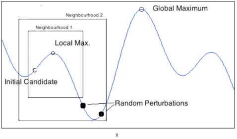
and Hansen (1997) is to subject an initial solution candidate to a sequence of local changes such that this effects an improvement in the value of an objective function after each iteration. The search is continued in this fashion until a (local) optimum is located. Initially, a

pre-defined neighbourhood,

_Ν

_i, having

i

neighbourhood structures is defined where the set

of solutions in the

i

th neighbourhood of x is given by

Ν

_i

( )

x

. A graphical illustration of the

principle behind the VNS method is provided in figure 1.

From the figure one can see how it is possible to combine both the EM and VNS algorithms. The resulting hybrid is termed the EMVNS algorithm and is described in detail by Bessadok et al. (2009). The novelty of the approach is to render the convergence of the EM routine independent of the initial starting – or candidate – solution. This may also help to overcome the problems posed by pathological likelihood functions with large attraction basins. In effect, the EMVNS uses the EM as a local search method that works in the larger context of a global optimization routine that seeks to maximize the log-likelihood function in order to obtain the model parameters. Under EMVNS, the maximization of the log-likelihood is performed under the condition that the estimated model parameters belong to the set of feasible neighbourhood solutions. As discussed in Bessadok et al. this means that the neighbourhood structures must be defined as subintervals derived from the observed distribution of the data.

In terms of its implementation, the EMVNS algorithm proceeds as follows. First, an initial

candidate solution

θ

is used to initialize the EM algorithm. An initial solution can be found

either by using a judicious choice of starting parameters or by an automatic initialization routine. For example, Biernacki et al. compare various methods for choosing the starting values of the EM algorithm for multivariate Gaussian mixture models. In terms of automatic

initialization schemes, one popular method makes use of the k-means clustering algorithm

proposed by Hartigan and Wong (1979). The aforementioned subinterval ranges of the

data, indicated by

I

_p, can be extracted from the respective sample statistics of the means,

covariances and mixing weight parameters of the input data. Next, the maximum number of

embedded intervals in

I

_p is specified which gives

I

_pk

,

k

=

1

,

2

,

_K

,

k

_max. Here k identifies a

given search neighbourhood. The algorithm’s complete pseudo code is provided in the accompanying box (1). By formulating the search in this manner, the complete set of neighbourhood structures is searched for local optima and, based on the convergence criteria, the algorithm selects the best solution within the set of feasible solutions in the search space.

Box 1: EMVNS algorithm pseudo code.

5. Data and Estimation of the SUR Model

The data consists of historical probabilities of default calculated on a quarterly basis over the period spanning the first quarter of 1995 until the third quarter of 2010 yielding a total of 63 observations. Along with the probability of default, the model incorporates data on the real growth rate of Luxembourg GDP, euro area real GDP growth, the real interest rate, the change in real property prices and the returns on the Euro Stoxx 50 (SX5E) index. This combination of variables allows for possible feedback effects between the probability of default series and the evolution of the macroeconomic variables. SUR estimation accounted for any contemporaneous correlation in the cross-equation residuals. A detailed description of the SUR model specification and its estimation is provided in Rouabah and Theal (2010). Since data on the aggregate default rate of Luxembourg banking sector counterparties was unavailable, it was necessary to construct the series of historical default probabilities. These default probabilities were calculated using a ratio of provisions on loans to total loans to all sectors. Subsequently, this ratio was used as an approximation for the aggregate sector probability of default. Although provisioning provides an estimate of the probability of default, it is important to recognize that loan loss provisions are, in effect, an imperfect approximation of default rates over the business cycle. More specifically, provisioning in some countries can be used for tax deductions and thus provisioning may only partially reflect credit risk concerns and the true degree of loan impairments. It is also important to

Repeat the following until the stopping condition is satisfied:

i. set k←1

ii. Repeat the following until

k

=

k

_max

a. Perturbation/shaking phase. Randomly draw a

parameter vector

θ

′ from the

_k

th _{neighbourhood of}

θ

where

θ

′

∈

I

_pk

( )

θ

;

b. Estimate the model using EM. Using

θ

′ as the

candidate solution, the EM algorithm is applied to

obtain a local optimum denoted by

θ

′′;

c. Return to (i). If the local optimum is an improvement

over the candidate, use this optimum so that

θ

←

θ

′′

and continue the search procedure setting

(

1

)

1

k

←

mention that loan loss provisions themselves can, in some cases, be used in order to adhere to regulatory capital requirements. Finally, both of these series are backward looking, so the results should be interpreted with caution. The coefficients of the estimated SUR model are reported in table 1.

[ Table 1 about here ]

The signs of the coefficients appear appropriate for the expected dependence of the probability of default on the selected macroeconomic variables. Positive increases in the

growth rates of euro area and Luxembourg GDP result in an increase in the variable y_t.

Since y_t is inversely related to the probability of default, this means that a decrease in euro

area or Luxembourg real GDP growth could result in a positive increase in the probability of default of Luxembourg banking sector counterparties. Furthermore, the magnitude of the coefficients suggests that this effect is strongly influenced by real GDP growth in the euro area. This is consistent with the interpretation that Luxembourg’s economy is sensitive to the fundamentals of the euro area economy. Increases in the real interest rate also demonstrate a strong effect on the creditworthiness of counterparties, illustrating that increases in the real rate of interest increase counterparty risk. Since the lagged coefficient

of y_t (i.e. y_t−1) is positive and highly significant, this suggests that autocorrelation in the

probability of default series will result in exogenous shocks persisting for a horizon that exceeds the duration of the shock. The same holds for many of the macroeconomic variable equations, suggesting the model can capture a dynamic response to an initial shock. Using Monte Carlo simulations as detailed in Rouabah and Theal (2010), it would be possible to use the same approach to simulate distributions of the counterparty probability of default with the MVAR model. In the context of the SUR model, this was done previously and an example is shown in figure (2).

[ Figure 2 about here ]

This figure compares the distribution of counterparty creditworthiness under the baseline and the adverse scenario.

6. Implementation of EMVNS and the Estimation of the MVAR Model

To estimate the MVAR model parameters, we implement the EMVNS algorithm using four neighbourhood structures within which we perturb the parameters. Given the nature of the MVAR model, the EMVNS convers the following neighbourhoods: 1) perturbation of the distribution mixing weights, 2) perturbation of the intercept vector, 3) perturbation of the autoregressive coefficient matrices and, 4) perturbations of the variance-covariance

matrices. The MVAR log-likelihood function has as its parameter set all the expressions in equation (9). Given the parameter set, this specification for the neighbourhood structures enables a thorough search of the parameter space of the log-likelihood function. This increases the likelihood that the EMVNS converges to the global maximum.

It is important to address a few idiosyncracies that are inherent in the empirical implementation and estimation procedure. First, the diagonal values of the variance-covariance matrix may need to be regularized in order to ensure it remains positive definite. We therefore calculate the condition number of the covariance matrix and add a small, positive value to the main diagonal of the matrix if necessary. The magnitude of this number is close to the empirical precision of the computer on which the code is executed. Second, to ensure a computationally efficient estimation procedure, one of our stopping conditions monitors the amount of CPU time consumed by a given iteration in the maximization phase of the algorithm. If convergence is not achieved within a pre-specified CPU time limit, the current iteration is terminated and the algorithm proceeds to the next iteration. We apply the same limit to the search of a given neighbourhood structure. In both cases, the time limit

employed is approximately 40 seconds6_.

We use a two-distribution mixture so results may be interpreted in terms of two regimes; one

for economic “good” times and the other for economic “bad” times. The entries for

τ

_t,k, the

conditional probability that a given observation originates from component k=1,2 of the distribution, suggest that component one probabilities are larger during so-called “good” economic periods, and component two probabilites tend to be associated with periods of economic stress, although this classification is not entirely rigorous. The actual number of observations associated with tranquil times is 30 compared to 28 associated with times of turmoil. The absence of a clearer distinction between good and bad times may be in part attributed to the increased volatility and short length of the time series data used in this work. Tables (2a) and (2b) provide the estimated coefficients and their respective standard errors for the MVAR model component distributions. It should be noted that the standard errors of

the MVAR coefficients were estimated using Louis (1982) method7_{. This is based on the}

6 _{At first glance, this limit may seem constraining. However, the algorithm was implemented in} MATLAB, an interpreter language, for which run-times tend to be slower than for compiled languages. An implementation using compiled binary code may substantially reduce this limit.

7 _{The procedure and equations for the estimation of the standard errors were obtained from C. S.} Wong in the form of a private communication of an unpublished manuscript.

empirical evaluation of both the observed information in Y and missing information in Z. In order to obtain these matrices it is necessary to evaluate the second derivatives of the

likelihood function8_{. In the case of the MVAR the second derivatives were derived}

analytically although for more complicated likelihood functions, these may not exist. In this case, second derivatives may be approximated numerically, although at the cost of lower numerical precision. In any case, once the second derivatives are known, the standard

errors can be extracted from the complete information matrix,

I

, which is defined as the

difference between the observed information and missing information matrices as given by equation (10). θ θ m c

θ

Y

θ

Y

θ

θ

θ

I

I

I

ˆ ˆ 2

,

var

,

_⎟⎟

⎠

⎞

⎜⎜

⎝

⎛

∂

∂

−

⎟⎟

⎠

⎞

⎜⎜

⎝

⎛

′

∂

∂

∂

=

−

=

E

l

l

(10)

The following variable definitions apply here: _l is the MVAR log-likelihood function,

Y

is the

observed data and θ contains the estimated model coefficients.

I

_c and I_m are the

complete information and missing information matrices, respectively.

[ Table (2a) about here ] [ Table (2b) about here ] [ Figure 3 about here ]

Figure 3 shows the convergence of the likelihood function. Although the number of iterations required to achieve convergence is fairly low, the curve remains monotonic. The EMVNS

algorithm required 24 iterations to converge9_.

Tables (2a) and (2b) provide some information on the dynamics and feedback mechanisms between the macroeconomic environment and the logit-transformed and differenced

probability of default series, _Δy_t. For the first component distribution (Table 2a), with the

exception of property prices, the signs of the coefficients in the first column seem appropriate for the expected link between the macroeconomic environment and the creditworthiness of Luxembourg’s banking sector counterparties. The coefficients for the change in property prices are not statistically significant, suggesting a high degree of

8 _{As these expressions are outside the scope of this work, they are not provided here.}

9_{Convergence was defined as an improvement in the log-likelihood function between two successive} iterations that is less than

1

_×

10

−6_.

uncertainty. This may reflect the small sample size or measurement error in the property price data. Specifically, this series is subject to large revisions and excludes non-residential property. As already mentioned, Virolainen (2004) encountered difficulties of a similar nature with his interest rate series; he appearerd unable to find an appropriate role for the real interest rate in his model. The coefficient on euro area GDP growth is positive and

significant. Since _Δy_t is inversely related to the probability of default, when euro area GDP

growth increases, the probability of default of the aggregated counterparties decreases. Coefficients on real GDP growth in Luxembourg and the property price index are not statistically significant. Neither is the coefficient on the change in the real interest rate, although it is negative, suggesting that when interest rates increase, counterparty creditworthiness as measured by the probability of default decreases (i.e. the PD measure

increases since if _Δy_t decreases, PD augments).

Looking at the other columns, euro area real GDP growth tends to increase when counterparty PDs recede. In addition, there is a persistence effect, as the coefficient of the lagged term in euro area GDP growth is statistically significant. The real interest rate appears to be linked to past changes in the property price index. Specifically, a decline in property prices in the previous period tends to decrease interest rates suggesting that favourable conditions in the last period lead to improved market conditions in the current period. In so far as Luxembourg property prices are correlated with those in the euro area, this result could be interpreted as a general symptom of favourable economic periods. Not unexpectedly, the dynamics under the second component (Table 2b) differ. Under this

regime, Luxembourg real GDP growth in the previous period results in an increase in _Δy_t

which reflects a decrease in counterparty risk as measured by PD. Additionally, there

seems to be some persistence in the dynamics for Δy_t. Lagged values of Δy_t up to two

previous periods previous are associated with positive changes in the logit-transformed series. The sum of autoregressive coefficients is greater than in Table 2a, suggesting more persistence under the second regime. Crisis period dynamics appear to be more volatile

since the autoregressive coefficient on

( )

EUR

t

g

₁

ln

₋

Δ

in column 2 is negative and significant.

The coefficient

( )

EUR

t

g

₁

ln

₋

Δ

is also large and negative in colum 3, suggesting a volatile impact

on Luxembourg GDP growth, in addition to significant persistence. In other words, it appears that Luxembourg’s real GDP growth is affected by developments in the larger euro area during periods of economic stress. The interest rate equation in column 4 also features significant persistence.

With respect to GDP for both Luxembourg and the euro area, there appears to be a feedback mechanism at work between property prices, Luxembourg GDP and counterparty

creditworthiness. Indeed, a rise in property prices at time t−1 leads to an increase in

Luxembourg real GDP growth. In turn, this implies a decline in the PDs of counterparties. However, this mechanism seems to have the opposite effect under the first component for euro area real GDP growth. In any case, there appears to be some persistence behind this effect as increasing property prices tend to result in favourable property prices in the next period. These findings suggest that the real estate sector may be a relevant indicator of economic performance in Luxembourg. Indeed, this result is consistent with Morhs (2010) who finds that there is a response of both credit and GDP to residential property price shocks in Luxembourg. Taken together, these results can be interpreted as evidence in favour of the existence of a house price channel of monetary policy transmission in Luxembourg.

Table 3 shows the estimated residual covariance matrices for the two components. These matrices are symmetric. The values of the covariance estimates are considerably small,

most being less than

1

_×

10

−5_{. However, there are three values in particular that are}

statistically significant. The variance of _Δy_t is 0.0056 and is significant. Similarly, the

covariance between _Δy_t and

Δ

p

_t is 0.005 and is highly significant. This result seems to

confirm the link between the property markets and the creditworthiness of banking sector

counterparties in Luxembourg. The variance of _Δy_t remains significant under the second

component distribution, but is smaller in magnitude having a value of 0.0002. Conversely, the link between the real estate price index and the change in counterparty creditworthiness is no longer significant. Overall, values in the second component distribution are smaller than those for the first component.

[ Table 3 about here ]

To demonstrate the improved ability of the MVAR model to capture extreme events, we can

estimate the predictive distributions, F

(

Z_{t ℑt−1}

)

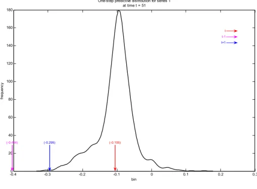
, at different time periods in the data sample.

Figure (4) shows the one-step ahead predictive distribution of the SUR model while figure (5) shows the associated predictive distribution of the MVAR model. Both are evaluated during Q4 of 2008, which was identified as a high point of stress during the recent financial crisis. In interpreting the figures, it is useful to recall that, under the logit transformation, a decrease in the transformed indicator represents an increase in the actual probability of default.

[ Figure 5 about here ]

The vertical red bars in the plots indicate the realized values of the change in the credit risk

indicator

( )

Δ

y

_t between period

t

and t+1. These quantities are -0.105 and -0.295,

respectively. For the univariate distribution, the predicted value of

Δ

y

_t at time t+1 appears

in the far left-hand tail of the distribution, whereas the equivalent point in the MVAR model’s predictive distribution is also captured in the tail of the distribution however its mean is not centred about zero. Rather, the mean value is close to -0.1 suggesting that, on average, increased values of the probability of default are more frequently observed in comparison to the SUR distribution. This elevation in the level of the probability of default is consistent with

a crisis situation. Furthermore, this implies that negative values of the indicator at time t+1

are more likely to occur under the MVAR model than under the univariate SUR model. In terms of counterparty creditworthiness, this means that the univariate distribution significantly underestimates the risk to credit quality. More specifically, the univariate model indicates that these elevated PD values are much less likely to occur compared to the prediction of the MVAR model. In addition, the distribution of the MVAR model assigns much more weight to negative movements in the credit risk indicator which corresponds to increases in the probability of default. In contrast, the univariate distribution appears to be much more symmetric about zero.

As a second example, figure (6) and figure (7) show the SUR and MVAR predictive

distributions for an alternate time,

t

. As in figures (4) and (5), there are clear advantages in

the prediction ability of the MVAR distribution compared to the SUR case.

[ Figure 6 about here ] [ Figure 7 about here ]

7. The Kullback-Leibler Measure of Divergence

The Kullback-Leibler divergence is an information theoretic quantity closely related to Fisher’s concept of a sufficient statistic. It is alternatively known as the information gain and was originally proposed by Kullback and Leibler (1951). This quantity is a non-symmetric measure, or “distance” in a heuristic sense, of the difference between the distribution of an observed sample population and what can be considered as the conceptual reality. However, it is not a distance in the true sense as the measure is non-symmetric (although a

and f

( )

_⋅ be the conceptual distribution, then the Kullback-Leibler divergence for continuous functions is given by the following integral:

( )

_∫

∞

( )

_{( )}

( )

∞ −

⎟

⎟

⎠

⎞

⎜

⎜

⎝

⎛

=

dx

x

g

x

f

x

f

g

f

I

_e

θ

log

,

(11)

In equation (11), f

( )

_⋅ and g

( )

_⋅ are n-dimensional probability distribution functions. In this

form, the Kullback-Leibler divergence can be interpreted as the amount of information lost

when g

( )

_⋅ is used to approximate the “true” model as given by f

( )

_⋅ . Note that in equation

(11) both f

( )

_⋅ and g

( )

_⋅ must be normalized to unity and g

( )

x

θ

>0 such that f

( )

x >0.

These conditions ensure that I

( )

f,g remains greater than or equal to zero. The

Kullback-Leibler divergence can be used for model selection since minimizing the distance over the choice of available models can be used as a selection criterion. Indeed, Akaike exploited this result for his well known Akaike information criterion (AIC). The Kullback-Leibler divergence is also used as a measure of information gain in Bayesian statistics when moving from the prior to the posterior distribution.

It is possible to calculate the KLD between the one-step ahead predictive distributions at various points in time. Positive values of KLD can be interpreted as the information gain of the MVAR distribution in comparison to that of the SUR model. The values of KLD at different time periods, both crisis and non-crisis, are shown in table (4). The results seem to show that the difference between the two measures of the Kullback-Leibler divergence remains relatively consistent, but significant differences appear during times of crisis. In particular, the MVAR-SUR KLD tends to become quite large in comparison to its historical average. This suggests that the MVAR predictive distribution exhibits an information gain in comparison to the SUR predictive distribution. This interpretation is consistent with the hypothesis that the MVAR model is able to better capture extreme movements in credit risk. This result seems to be confirmed by the index of vulnerability published by in the Financial Stability Review (FSR) of the Banque centrale du Luxembourg. Indeed, the vulnerability index in the 2011 FSR exhibits a period of intense vulnerability over the period spanning from the second quarter of 2008 until the last quarter of 2009. This corresponds to the period in which the difference between the MVAR-SUR and SUR-MVAR KLD difference deviates strongly from its historical average. It could be interesting to pursue additional metrics for gauging the difference between the two distributions in order to confirm that this is a reliable result. Unfortunately, at the moment there are no tests that are capable of

gauging the degree of statistical significance of these results. We consider this a potential avenue for future research.

Conclusion

Taken together, these results suggest that, compared to a framework with a unimodal distribution, using the MVAR model to assess counterparty risk provides a more accurate representation of the true risk by better capturing the more extreme movements observed in empirical measures of credit risk. Furthermore, using the Kullback-Leibler divergence as a measure of the “bias” between the predictive distributions of the MVAR and SUR models seems to be able to identify periods of crisis. This may demonstrate that there is an information gain provided by the MVAR model which is not present in the SUR framework. However, at this time there is no statistical test that we can apply to these results to gauge their significance.

The next step in our research is to extend the MVAR work in order to simulate baseline and adverse distributions of the probability of default and compare these to a VAR model. This would allow us to quantify the gap between the MVAR and VAR model results under both stressed and benign economic conditions and, in turn, to assess the resulting impact on the capital requirements for banks in a manner similar to those obtained from the SUR model.

References

Bessadok, A., P. Hansen and A. Rebaï. (2009). “EM algorithm and Variable Neighborhood

Search for fitting finite mixture model parameters,” Proceedings of the International

Multiconference on Computer Science and Information Technology, Vol. 4, pp. 725-733. Biernacki, C., G. Celeux and G. Govaert. (2003). “Choosing starting values for the EM algorithm for getting the highest likelihood in multivariate Gaussian mixture models,”

Computational Statistics & Data Analysis, Vol. 41, Issues 3-4, pp. 561-575.

Borio, C. (2010). “Implementing a macroprudential framework: Blending boldness and

realism”, Bank for International Settlements.

Borio, C. (2009). “Implementing the macroprudential approach to financial regulation and

supervision”, Financial Stability Review, Banque de France, No. 13, pp. 31-41.

Dempster, A. P., N. M. Laird and D. B. Rubin. (1977). “Maximum Likelihood from Incomplete

Data via the EM Algorithm,” Journal of the Royal Statistical Society. Series B

(Methodological), Vol. 39, No. 1. pp. 1-38.

Filosa, R. (2007). “Stress testing of the stability of the Italian banking system: a VAR

approach”, Working Paper.

Fong, P. W., W. K. Li, C. W. Yau and C. S. Wong. (2007). “On a mixture vector

autoregressive model”, The Canadian Journal of Statistics, Vol. 35, No. 1, pp. 135-150.

Fong, T. P. and C. Wong. (2008). “Stress testing banks’ credit risk using mixture vector

autoregressive models,” Hong Kong Monetary Authority, Working Paper 13/2008.

Hartigan, J. A., and M. A. Wong. (1979). “A K-Means Clustering Algorithm,” Journal of the

Royal Statistical Society. Series C (Applied Statistics), Vol. 28, No. 1, pp. 100-108.

Hoggarth, G., Steffen Sorensen and Lea Zicchino. (2005). “Stress tests of UK banks using a

VAR approach”, Bank of England Working Paper, November.

Huang, X., H. Zhou, and H. Yhu. (2009). “A framework for assessing the systemic risk of

major financial institutions”, Journal of Banking and Finance, Vol. 33, pp. 2036-2049.

Kullback, S. and R. A. Leibler. (1951). “On information and sufficiency.” Annals of

Mathematical Statistics. Vol. 22, pp. 79-86.

Louis, T. A. (1982). “Finding the observed information matrix when using the EM algorithm,”

Journal of the Royal Statistical Society. Series B (Methodological), Vol. 44, No. 2, pp. 226-233.

Maciejowska, K. (2010). “Estimation methods comparison of SVAR model with the mixture of

two normal distributions – Monte Carlo analysis,” EUI Working Papers, European University

McLachlan, G. J. and T. Krishnan. (2008). “The EM Algorithm and Extensions,” Second Edition, John Wiley & Sons, Inc. Hoboken, New Jersey.

Mladenović, N. and P. Hansen. (1997). “Variable Neighborhood Search,” Computers &

Operations Research, Vol. 24, No. 11, pp. 1097-1100.

Morhs, R. (2010). “Monetary policy transmission and macroeconomic dynamics in

Luxembourg: Results from a VAR analysis,” Banque central du Luxembourg, Working Paper

No. 49.

Rouabah, A. and J. Theal. (2010). “Stress Testing: The Impact of Shocks on the Capital

Needs of the Luxembourg Banking Sector”, Banque centrale du Luxembourg, Working

Paper No. 47.

Sorge, M. (2004). “Stress-testing financial systems: an overview of current methodologies,”

BIS Working Papers, No. 165.

Virolainen, K. (2004). “Macro stress testing with a macroeconomic credit risk model for

Finland”, Bank of Finland Discussion Papers, No. 18.

Wilson, T. C. (1997a). “Portfolio Credit Risk (I),” Risk, vol. 10, issue 9, pp. 111-117.

Wilson, T. C. (1997b). “Portfolio Credit Risk (II),” Risk, vol. 10, issue 10, pp. 56-61.

Wong, C. S. and W. K. Li. (2000). “On a mixture autoregressive model,” Journal of the Royal

Statistical Society. Series B (Statistical Methodology), Vol. 62, No. 1, pp. 95-115.

Wong, J., K. Choi and T. Fong. (2006). “A framework for stress testing banks’ credit risk,”

Hong Kong Monetary Authority, Research Memorandum 15/2006.

Yan, Y., P. Barry, N. Paulson, and G. Schnitkey. (2009). “Measurement of farm credit risk:

SUR model and simulation approach,” Selected Paper prepared for presentation at the

Agricultural & Applied Economics Association 2009 AAEA & ACCI Joint Annual Meeting, Milwaukee, WI

Figure 1: Illustration of the EMVNS search procedure

Figure 2: Probabilities of default simulated from the SUR model: Baseline and adverse scenarios under shocks to the real interest rate

0 100 200 300 400 500 600 700 800 900 1000 0.42 0.56 0.7 0.84 0.98 1.12 1.26 1.4 1.54 1.68 1.82 1.96 2.1 2.24 2.38 2.52 2.66 2.8 2.94 3.08 3.22 3.36 3.5 3.64 3.78 3.92 Probability of Default (%) Fr eq ue n cy

Figure 3: Convergence of the MVAR log-likelihood function under the EM algorithm

Figure 4: Credit risk indicator predictive distribution for the SUR model during the last quarter of 2008. -0.40 -0.3 -0.2 -0.1 0 0.1 0.2 0.3 0.4 10 20 30 40 50 60 70 80 90

One-step predictive distribution for series 1 at time t = 51 bin fr eque nc y t t-1 t+1 (-0.105) (-0.404) (-0.295)

Figure 5:Credit risk indicator predictive distribution of the MVAR model for the fourth quarter of 2008. -0.40 -0.3 -0.2 -0.1 0 0.1 0.2 0.3 20 40 60 80 100 120 140 160 180

One-step predictive distribution for series 1 at time t = 51 bin fr eque nc y t t-1 t+1 (-0.105) (-0.404) (-0.295)

Figure 6: Credit risk indicator distribution for the SUR model

Univariate Model Predictive Distribution

0 100 200 300 400 500 600 700 -0,6 -0,4 -0,2 0 0,2 0,4 Value Fr equency t+1 = -0,165 _{t = -0,047}

Figure 7: Credit risk indicator distribution for the MVAR model

MVAR Model Predictive Distribution

0 100 200 300 400 500 600 700 -0,6 -0,4 -0,2 0 0,2 0,4 Value Fr eque nc y t+1 = -0,165 t = -0,047

Table 1:

Results of the SUR system estimation for the period 1995 Q1 to 2010 Q3

Dependent Variable Variable y_t

( )

EUR t

g

ln

Δ

( )

LUX t

g

ln

Δ

r_t Δp_t

Δ

ln

(

sx

5

e

_t

)

intercept 0.301*** 0.003*** 0.017*** _{0.002 0.008}

( )

EUR t

g

₁

ln

₋

Δ

4.477*** 0.521***

( )

EUR t

g

₂

ln

₋

Δ

-0.059

( )

EUR t

g

₄

ln

₋

Δ

-0.331

( )

LUX t

g

₁

ln

₋

Δ

0.615***

( )

LUX t

g

₃

ln

₋

Δ

0.533** r_t -0.140 r_t−1 -0.335 0.933*** r_t−4 -3.513*** Δp_t 0.550*** Δp_t−1 0.981*** y_t−1 0.934***

(

5

1

)

ln

₋

Δ

sx

e

t 0.034*** 0.857***

R

2 _{0.984 0.527 0.662 0.820 0.919 0.768} No. of obs. 56 59 58 59 58 59 Notes:

1. In the equations for

Δ

ln

( )

g

_tEUR and Δp_t, dummy variables have been added in order to control for structural breaks.