Prediction on Large Scale Data Using
Extreme Gradient Boosting
Thesis submitted in partial fulfillment of the requirement for the degree of
Bachelor of Computer Science and Engineering
Under the Supervision of
Moin Mostakim
By
Md.Tariq Hasan Sawon (11201030)
Md. Shazzed Hosen (11221039)
School of Engineering and Computer Science
August 2016
Page2of45
Declaration
We, hereby declare that this thesis is based on the results found by our own task.
Materials of work found by other researcher are mentioned by reference. This Thesis, neither in whole or in part, has been previously submitted to any other University or any Institute for the award of any degree or diploma.
Signature of the Supervisor Signature of Author
____________________________ ___________________________ Moin Mostakim Md. Tariq Hasan Sawon
___________________________ Md. Shazzed Hosen
Acknowledgement
Firstly, all praise to the Great Allah for whom our thesis have beencompleted without any major interruption.Secondly, we want thank our supervisor Mr. Moin Mostakim Sir for his kind support and advice in our work. He helped us whenever we needed help.Thirdly, we want to thank those entire respectable faculty members who gave us advice and suggestions time to time. All the reviews they gave helped us a lot in our later works.And finally to our parents without their throughout support it may not be possible. With their kind support and prayer were now on the verge of our graduation.
Page4of45
Contents
DECLARATION……….02 ACKNOWLEDGEMENTS………03 CONTENTS ………...04 LIST OF FIGURES..……….06 LIST OFTABLES………...07 LIST OF ABBRIVIATIONS…….………..08 ABSTRACT.……….. 09 CHAPTER 1: INTRODUCTION………...10 1.1Motivations ………11 1.2 Problem definition .……….…. 12 CHAPTER 2: BACKGROUND ..……….12 2.1Related Work………132.1.1 Microsoft Time Series Algorithm…..……… 14
2.1.2 Spatial data mining for retail sales forecasting……….15
2.1.3 A Novel Trigger Model for Sales Prediction with Data Mining Techniques………15
CHAPTER 3: SUPERVISED LEARNINING……….. 15
3.1 Generalizations of supervised learning... ...17
CHAPTER 4: Gradient descent..………...18
4.1 Extreme Gradient Boost (XGBoost)………..20
4.2 Gradient Boosting……….21
4.2.1 Objective function of XGBoost………22
CHAPTER 5: Dataset and Features ... 23
5.2 Detecting Trends ...24
5.3 Feature Relative Importance Estimation ...25
5.4 Missing Data ... 26
5.5 Data Collection...26
5.6 Dataset... 27
5.7 Data Field... 27
5.8 Data visualization and analysis ...28
Chapter 6: Machine learning algorithms and approaches ...35
Chapter 7: Results ...37
7.1 Prediction Modelling using Decision Tree ...38
7.2 Tools and Platforms... 38
7.3 Challenges... 39
7.4 Learnings ...39
7.5 Future works ...39
7.6 CONCLUSION ...40
Page6of45
LIST OF FIGURES
Figure 01: Finding the gradient of cost function ... 19
Figure 02: Trajectory of Gradient descent through cost function ... 20
Figure 03: Overfitting and regularization 23
Figure 4: Depicts the histogram of the mean sales per storewhenthe stores weren’t closed . 24
Figure 5: Distribution among all sales (left side); logarithm of it (right side) ... 32
Figure 6: Amount of days by weeks and by years among all stores ... 33
LIST OF TABLES
Table 1: Store data representation ...28
Table 2: Train data representation ...29
Table 3: Store data representation ...30
Table 4: Column by files of given Dataset ...30
Table 5: Simple data information ...31
Page8of45
LIST OF ABBRIVIATIONS
XGBoost: Extreme Gradient Boosting
RMSPE: Root Mean Square Percentage Error
ARTXP: Autoregressive Tree Models with Cross Prediction
ARIMA: Autoregressive Integrated Moving Average
SVR: Support Vector Regression
CVS: coefficient of variation for sales
CVA: Coefficient ofvariation for attention
SPV: Sold Price Variation
CART: Classification and regression trees
OOB: Out-of-bag
Abstract
This paper presents a use case of data mining for sales forecasting in retail demand and sales prediction. In particular, the Extreme Gradient Boosting algorithm is used to design a prediction model to accurately estimate probable sales for retail outlets of a major European Pharmacy retailing company. The forecast of potential sales is based on a mixture of temporal and
economical features including prior sales data, store promotions, retail competitors, school and state holidays, location and accessibility of the store as well as the time of year. The model building process was guided by common sense reasoning and by analytic knowledge discovered during data analysis and definitive conclusions were drawn. The performances of the XGBoost predictor were compared with those of more traditional regression algorithms like Linear
Regression and Random Forest Regression. Findings not only reveal that the XGBoost algorithm outperforms the traditional modeling approaches with regard to prediction accuracy, but it also uncovers new knowledge that is hidden in data which help in building a more robust feature set and strengthen the sales prediction model.
Page10of45
Chapter I: Introduction
Retail is one of the most important business domains for data science and data mining
applications because of its prolific data and numerous optimization problems such as optimal prices, discounts, recommendations, and stock levels that can be solved using data analysis methods. The usual problems tackled by data mining applications are Response Modeling, Recommendations systems, Demand prediction, Price Discrimination [12], Sales Event Planning, and Category Management [1]. Accurate forecasting of customer demand remains a
challenge in today’s competitive and dynamic business environment and minor improvements in predicting this demand helps diversified retailers lower operating costs while improving sales and customer satisfaction Predicting the right demand at each retail outlet is crucial for the success of every retailing company because it helps towards inventory management, results in better distribution of produce across stores, minimizes over and under stocking at each store thereby minimizing losses, and most importantly maximizes sales and customer satisfaction[3]. Due to the high stakes involved with demand prediction, it becomes a vital problem to solve for every retail company [19]. Further, demand can depend on a variety of external factors like competition, weather, seasonal trends, etc. and internal actions like promotions, sales events, pricing, assortment planning etc., adding to the complexity of the problem. Consequently, the modeling of demand prediction taking into account all of the factors per retail outlet becomes essential for everyretail company. Therefore, this paper proposes an approach for demand and sales prediction for retail at each outlet. Having fixed on the data mining problem of Sales prediction at each outlet of a retailing company, Rossmann -Germany’ssecond-largest drug
store chain with 3,000 stores in Europe, was chosen as the retailing company for data to develop the predictive model on. The data was available through their first Kaggle competition. In the competition Rossmann challenged to predict 6 weeks of daily sales for 1115 of their stores located across Germany. This is a crucial problem for Rossmann as currently their store
managers are tasked with predicting their daily sales for up to six weeks in advance. Since store sales are influenced by many factors, including promotions, competition, school and state holidays, seasonality, and locality and with thousands of individual managers predicting sales based on their unique circumstances, the accuracy of results has been quite varied. Therefore reliable sales forecasts will enable their store managers to create effective staff schedules that increaseproductivity and motivation.Rossmann is a chain drug store that operates in 7 European countries. We obtained Rossmann 1115Germany stores’ sales data from Kaggle.com. The goal
of this project is to have reliable sales prediction for each store for up to six weeks in advance. The topic is chosen, because the problem is intuitive to understand. We have a well
understanding of the problem from our daily life, which makes us more focused on training methodology. The input to our algorithm includes many factors impacting sales, such as store type, date, promotion etc.The result is to predict 1115 stores’ daily sale numbers. Extreme used to train model and predict sales.
1.1 Motivation
Rossmann store managers are tasked with predicting their daily sales for up to six weeks in advance. Store sales are influenced by many factors, including promotions, competition, school and state holidays, seasonality, and locality. With thousands of individual managers predicting sales based on their unique circumstances, the accuracy of results can be quite varied.
Page12of45
1.2 Problem definition
We are given dataset from Rossman inc. They ask us to write an algorithm that will predict quantity of sales in each of next 48 days. The evaluation metric for this problem is RSMPE. The RSMPE calculated as follows:
Where Yi - denotes the sales of a single store on a single day and ‘I’denotes the corresponding prediction. Any day and store with 0 sales is ignored in scoring. We challenged to predict continuous variable. To be explicit, we should predict field Sales.
Chapter II: Background
This background is driven by the current knowledge on gradient boosting that can be found in the literature. It first describes the original algorithm, details some commonly used loss functions and presents a general method of constructing regression trees. It then exposes the different
theories the scientific community developed to explain the gradient boosting’s behavior
regarding the overfitting phenomenon, and finishes by describing the state-of-the art approach to gradient boosting.
2.1 RELATED WORK
2.1.1 Microsoft Time Series Algorithm[2]: The Microsoft Time Series algorithm provides
regression algorithms that are optimized for the forecasting of continuous values over time. The major advantage of the Time Series Algorithm is that it does not require additional columns of new information as input to predict a trendwhereas other algorithms based on decision trees them. A time series model can predict trends based only on the original dataset that is used to create the model. Any new data added to the model when making a prediction is automatically incorporated into the trend analysis. Another unique feature of the Microsoft Time Series
algorithm is that it can perform cross prediction. The algorithm can be trained with two separate, but related, series, and the resulting model created can predict the outcome of one series based on the behavior of the other series. For example, the observed sales of one product can influence the forecasted sales of another product. How it Works: The Microsoft Time Series algorithm uses both methods, ARTXP (Autoregressive Tree Models with Cross Prediction) and ARIMA (Autoregressive Integrated Moving Average), and blends the results to improve prediction accuracy. The ARTXP algorithm can be described as an autoregressive tree model for representing periodic time series data. The ARIMA algorithm improves long-term prediction capabilities of the Time Series algorithm.
2.1.2 Spatial data mining for retail sales forecasting[13]:
This paper presents a use case of spatial data mining for aggregate sales forecasting in retail location planning. Support Vector Regression (SVR) is the technique used to design a regression model to predict probable turnovers for potential outlet-sites of a big European food retailing
Page14of45
company. The forecast of potential sites is based on sales data on shop level for existing stores and a broad variety of spatially aggregated geographical, socio-demographical and economical features describing the trading area and competitor characteristics. The model was built from a-priori expert knowledge and by analytic knowledge which was discovered during the data
mining process. To assess the performance of this SVR-model, it was compared to the traditional state-ofthe-artgravitational Huff-model. The spatial data miningmodel was found to outperform the traditional modelingapproach with regard to prediction accuracy. SupportVector algorithms are specially designed to minimize the expected classification error by minimizing both the empirical error and complexity. SVR works on almost the same principles as the Support Vector Classification. The SV-approach searches for the linear classifier which separates the positive from the negative instances of the training set by maximizing the margins. The margin
is the distance between the separating line and the nearest data points (the Support Vectors). This linear classifier is called the Optimal Separating Hyperplane. Kernel functions are used to handle instances where the data points are not linearly separable which works by transforming the input space containing the training instances into a new, higher-dimensional feature space, in which it becomes possible to separate the data.
2.1.3 A Novel Trigger Model for Sales Prediction with Data Mining Techniques[8]:
This paper describes anapproach on how to forecast sales with higher effectivenessand more accurate precision. The data used in thisapproach focuses on online shopping data in the
ChineseB2C market. The paper delves into e-commerce[17] andapplies real sales data to several classical predictionmodels, aiming to discover a trigger model that could selectthe appropriate
forecasting model to predict sales ofa given product. The paper aims to effectively support anenterprise in making sales decisions in actual operations.The approach involves manipulating raw data into availableforms and then a trigger model is proposed to do theclassification. The classification result indicates the bestprediction model for each item. Finally, by use of themost appropriate model, the prediction is accomplished.The features used are - CV Sales (CVS): coefficient of variation for sales , CV Attention (CVA): coefficient ofvariation for attention , Sold Price Variation (SPV): thevariation of sold price. This approach involves applyingtwo typical forecasting models and several dimensionsto the trigger model through training and testing theclassification model with real sales data and focuses onthe correlation of two subjects and ignores the causalrelationship between them.
Chapter III: Supervised Machine Learning
Supervised learning is the machine learning task of inferring a function from supervised training data. The training data consist of a set of training examples. In supervised learning, each example is a pair consisting of an input object (typically a vector) and a desired output value (also called the supervisory signal). A supervised learning algorithm analyzes the training data and produces an inferred function, which is called a classifier (if the output is discrete, see classification) or a regression function (if the output is continuous, see regression). The inferred function should predict the correct output value for any valid input object. This requires the learning algorithm to generalize from the training data to unseen situations in a "reasonable" way (see inductive bias).The parallel task in human and animal psychology is often referred to as concept learning. The majority of practical machine learning uses supervised learning.Supervised
Page16of45
learning is where you have input variables (x) and an output variable (Y) and you use an algorithm to learn the mapping function from the input to the output.
Y = f(X)
The goal is to approximate the mapping function so well that when you have new input data (x) that you can predict the output variables (Y) for that data.It is called supervised learning because the process of algorithm learning from the training dataset can be thought of as a teacher
supervising the learning process. We know the correct answers; the algorithm iteratively makes predictions on the training data and is corrected by the teacher. Learning stops when the
algorithm achieves an acceptable level of performance.Supervised learning problems can be further grouped into regression and classification problems.
Classification: A classification problem is when the output variable is a category, such as
“red” or “blue” or “disease” and “no disease”.
Regression: A regression problem is when the output variable is a real value, such as
“dollars” or “weight”.
Some common types of problems built on top of classification and regression include
recommendation and time series prediction respectively.Some popular examples of supervised machine learning algorithms are:
Linear regression for regression problems.
Random forest for classification and regression problems.
3.1 Generalizations of supervised learning
There are several ways in which the standard supervised learning problem can be generalized:
Semi-supervised learning: In this setting, the desired output values are provided only for a subset of the training data. The remaining data is unlabeled.
Active learning: Instead of assuming that all of the training examples are given at the start, active learning algorithms interactively collect new examples, typically by making queries to a human user. Often, the queries are based on unlabeled data, which is a scenario that combines semi-supervised learning with active learning.
Structured prediction: When the desired output value is a complex object, such as a parse tree or a labeled graph, then standard methods must be extended.
Learning to rank: When the input is a set of objects and the desired output is a ranking of those objects, then again the standard methods must be extended.Page18of45
Chapter IV: Gradient descent
Gradient descent is a method of searching for model parameters which result in the best fitting model. There are many search algorithms but this one is quick and efficient for many sorts of supervised learning models.Let's take the simplest of simple regression models for predicting y=α+βx
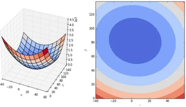
Our model has two parameters α, the intercept and β, the coefficient for xand we want to find the values which produce the best fitting regression line.How do we know whether one model fits better than another? We calculate the error or cost of the predictions. For regression models, the most common cost function is mean squared error:
Cost = J(α,β)=12n∑(y^−y)2=1n∑(α+βx−y)2
The cost function quantifies the error for any given αand β. Since it is squared, it will take the
form of an inverted parabola. Let's visualise what it looks like for the first 100 observations in our dataset:
Figure 01: Finding the gradient of cost function
At the bottom (or minima) or the parabola is the lowest possible cost. We want to find the α and βwhich correspond to that minima.The idea of gradient descent is to take small steps down the
surface of the parabola until we reach the bottom. The gradient of gradient descent is the gradient of the cost function, which we find by taking the partial derivative of the cost function with respect to the model coefficients.
Steps:
For the current value of αand β,calculate the cost and the gradient of the cost function at that point.Update the values of αand β by taking a small step towards the minima. This means,
subtracting some fraction of the gradient from them. The formulae are:
α=α−γ∂J(α,β)∂α=α−γ1n∑2(α+βx−y)
β=β−γ∂J(α,β)∂β=β−γ1n∑2x(α+βx−y)
Figure 01: Finding the gradient of cost function
At the bottom (or minima) or the parabola is the lowest possible cost. We want to find the α and βwhich correspond to that minima.The idea of gradient descent is to take small steps down the
surface of the parabola until we reach the bottom. The gradient of gradient descent is the gradient of the cost function, which we find by taking the partial derivative of the cost function with respect to the model coefficients.
Steps:
For the current value of αand β,calculate the cost and the gradient of the cost function at that point.Update the values of αand β by taking a small step towards the minima. This means,
subtracting some fraction of the gradient from them. The formulae are:
α=α−γ∂J(α,β)∂α=α−γ1n∑2(α+βx−y)
Page20of45
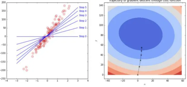
Steps 1 & 2 are repeated until one is satisfied that the model is not getting any better (cost isn't decreasing much with each step).The learning rate parameter γcontrols the size of the steps. This
is a parameter which we must choose. There is some art in choosing a good learning rate, for if it is too large or too small then it can prevent the algorithm from finding the minima.
Left chart: see how the regression line is gradually finding its way to fitting the shape of the
data? Right chart: the gradient descent algorithm moves toward lower cost values for α and β.
Figure 02: Trajectory of Gradient descent through cost function
4.1 Extreme Gradient Boost (XGBoost)
XGBoost is a library designed and optimized for boosting trees algorithms. Gradient boosting trees model is originally proposed by Friedman et al. The underlying algorithm of XGBoost is similar. Specifically, it is an extension of the classic gbm algorithm. It is used for supervised learning problems, where we use the training data (with multiple features) xi to predict a target
Page20of45
Steps 1 & 2 are repeated until one is satisfied that the model is not getting any better (cost isn't decreasing much with each step).The learning rate parameter γcontrols the size of the steps. This
is a parameter which we must choose. There is some art in choosing a good learning rate, for if it is too large or too small then it can prevent the algorithm from finding the minima.
Left chart: see how the regression line is gradually finding its way to fitting the shape of the
data? Right chart: the gradient descent algorithm moves toward lower cost values for α and β.
Figure 02: Trajectory of Gradient descent through cost function
4.1 Extreme Gradient Boost (XGBoost)
XGBoost is a library designed and optimized for boosting trees algorithms. Gradient boosting trees model is originally proposed by Friedman et al. The underlying algorithm of XGBoost is similar. Specifically, it is an extension of the classic gbm algorithm. It is used for supervised learning problems, where we use the training data (with multiple features) xi to predict a target
variable yi. It is similar to gradient boosting framework but more efficient. It has both linear model solver and tree learning algorithms. This makes xgboost at least 10 times faster than existing gradient boosting implementations. It supports various objective functions, including regression, classification and ranking. Since it is very high in predictive power but relatively slowwith implementation, “xgboost” becomes an ideal fit for many competitions. It also has
additional features for doing cross validation and finding important variables. There are many parameters which need to be controlled to optimize the model.While looking at better techniques for data analysis and forecasting online, we came across XGBoost which gives much better performance results than Linear Regression or Random Forest Regression. XGBoost [5] or Extreme Gradient Boosting is a library that is designed, and optimized for boosted (tree) algorithms. The library aims to providea scalable, portable and accurate framework for large scale tree boosting. It is an improvement on the existing Gradient Boosting technique.
4.2 Gradient Boosting:
Gradient boosting [7] is a machine learning technique for regression and classification problems, which produces a prediction model in the form of weak prediction models, typically decision trees. Boosting can be interpreted as an optimization algorithm on a suitable cost function. Like other boosting methods, gradient boosting combines weak learners into a single strong learner, in an iterative fashion. XGBoost is used for supervised learning problems, where we use the
training data x to predict a target variable y. The regularization term controls the complexity of the model, which helps us to avoid overfitting. XGBoost is built on a Tree Ensemble model which is a set of classification and regression trees (CART). We classify the members of a family into different leaves, and assign them the score on corresponding leaf. The main difference between CART and decision trees is that in CART, a real score is associated with
Page22of45
each of the leaves in addition to the decision value. This gives us richer interpretations that go beyond classification. It consists of 3 steps
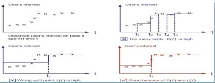
-1) Additive Training: In this stage we define the parameters of trees which are those functions that contain information about the structure of the tree and the leaf score.This is optimized by using an additive strategy: fix what we have learned, add a new tree at a time.
2) Model Complexity: The complexity of the tree acts as our regularization parameter and helps decide how to penalize certain cases.
3) Structure Score: This score is gives information on the best split conditions while taking the model complexity into account. The first split of a tree will have moreimpact on the purity and the following splits focus on smaller parts of the dataset which have been misclassified by the first tree.
4.2.1 Objective function of XGBoost
1st term of objective function is training loss function which measures how predictive our model is.
2nd term is regularization term which helps us to overfitting the data.Page22of45
each of the leaves in addition to the decision value. This gives us richer interpretations that go beyond classification. It consists of 3 steps
-1) Additive Training: In this stage we define the parameters of trees which are those functions that contain information about the structure of the tree and the leaf score.This is optimized by using an additive strategy: fix what we have learned, add a new tree at a time.
2) Model Complexity: The complexity of the tree acts as our regularization parameter and helps decide how to penalize certain cases.
3) Structure Score: This score is gives information on the best split conditions while taking the model complexity into account. The first split of a tree will have moreimpact on the purity and the following splits focus on smaller parts of the dataset which have been misclassified by the first tree.
4.2.1 Objective function of XGBoost
1st term of objective function is training loss function which measures how predictive our model is.Figure 03: Overfitting and regularization
Chapter V: Dataset and Features
Training data is comprised of two parts. One part is historical daily sales data of each store from 01/01/2013 to 07/31/2015. This part of data has about 1 million entries. Data included multiple features that could impact sales. Table 1 describes all the fields in this training data.
5.1 Data Description
We collected data from different data warehouse. We had chosen Rossmann drug store’s sales
data which is the second largest drug store in Germany. We implemented Extreme Gradient Boost to predict the daily sales for 6 weeks into the future for more than 1,000 stores. The
Rossmann Data contains information about 1115 stores from 1st Jan 2013 to 31st July 2015 (942 days). In total we have 1017209 entries[16].
Figure 03: Overfitting and regularization
Chapter V: Dataset and Features
Training data is comprised of two parts. One part is historical daily sales data of each store from 01/01/2013 to 07/31/2015. This part of data has about 1 million entries. Data included multiple features that could impact sales. Table 1 describes all the fields in this training data.
5.1 Data Description
We collected data from different data warehouse. We had chosen Rossmann drug store’s sales
data which is the second largest drug store in Germany. We implemented Extreme Gradient Boost to predict the daily sales for 6 weeks into the future for more than 1,000 stores. The
Rossmann Data contains information about 1115 stores from 1st Jan 2013 to 31st July 2015 (942 days). In total we have 1017209 entries[16].
Page24of45 Figure 4: depicts the histogram of the mean sales per storewhenthe stores weren’t closed.
From this graph we can infer thatmost stores have very similar sales and that there is a
smallpercentage of outliers. Average sales tend to be more on the Sunday as compared to other days. However, the magnitude of customers visiting a store on weekends tends to be less due to the fact that most stores are closed on Sunday.
5.2 Detecting Trends:
Using services such as Google Trends makes it easy to visualize the data and draw conclusions from it. It helps by giving information on external conditions which explain certain outliers in the training data. For example analyzing Weather data[14] gives a good idea (heavy snowfall) on why certain stores in a geographical area had lower sales at certainweeks of the year. It also indicated that Pre-holiday sales are higher in stores as opposed to sales on a normal day. This could be due to promo offers being run during the holiday period. Also state holidays vary by
date from state to state In addition data was looked into for the following Geographical and Social Factors -1) Accessibility 2) Store Location 3) Store Competition 4) Population Density
5.3 Feature Relative Importance Estimation
Decision tree is known for its ability to select “important”features among many and ignore (often irrelevant) others. In addition, decision tree gives an explicit model describing the
relationship between features and predictions, thus easingmodel interpretation. Random forest, as an ensemble of trees,inherits the ability to select “important” features. However, it does not produce an explicit model. Instead, the relationship between features and activity of interest is
hidden inside a“black box”. Nonetheless, a measure of how each featurecontributes to the
prediction performance of random forestcan be calculated in the course of training. When a feature that contributes to prediction performance is “noised up” (e.g.,replaced with random noise), the performance of prediction is noticeably degrade. On the other hand, if a feature is irrelevant,“noising” it up should have little effect on the performance. Thus, we can estimate the relative importance of features according to the followingprocedure[18]. As each tree is grown, it makes predictions on the OOB (out-of-bag) data for that tree. At the same time, each feature in the OOB data is randomly permuted, one at a time, and each such modified dataset is also
Page26of45
predicted by a tree. At the end of the model training process, RMPSEs are calculated based on the OOB prediction as well as the OOB predictions with each features permuted. Let M be the RMPSE based on the OOB prediction and Mj the RMSE based on the OOB prediction with the jthfeature permuted. Then the measure of importance for the jthfeature is simply Mj− M.
5.4 Missing Data:
There are 180 stores missing 184 days of data in the middle of the series between 1 July 2014 to 31 Dec 2014
5.5 Data Collection
Collection of a large dataset is the main perspective of a data mining and machine learning research and collecting data with proper understanding from reliable source is most important. In our research, we needed a strong and reliable data source which we found in Kaggle. In 2010, Kaggle was founded as a platform for predictive modelling and analytics competitions on which companies and researchers post their data and statisticians and data miners from all over
theworld compete to produce the best models. There are lots of different kinds of formats of data and statistics however we have our own format of data collection in order to design our
5.6 Dataset
Sample data Set of Rossmann Drug Stores on sales has been given below:
TRAIN.CSV - historical data including sales
TEST.CSV - historical data excluding sales
STORE.CSV - supplemental information describing each of the stores
5.7 Data Field
Id - represents a (Store, Date) duple within the test set
Store - Unique Id for each store
Sales - The turnover for any given day (variable to be predicted)
Customers - The number of customers on a given day
Open - An indicator for whether the store was open: 0 = closed, 1 = open
StateHoliday - Indicates a state holiday. Normally all stores with few exceptions are closed on state holidays.All schools are closed on public holidays and weekends.
a = public holiday
b = Easter holiday
c = Christmas
0 = None
SchoolHoliday - Indicates if the (Store, Date) was affected by the closure of public schools.
Page28of45
Assortment - Describes an assortment level: a = basic, b = extra, c = extended
CompetitionDistance - Distance in meters to the nearest competitor store
CompetitionOpenSince [Month/Year] - Approximate year and month of the time the nearest competitor was opened
Promo - Indicates whether a store is running a promo on that day
Promo2 - Continuing and consecutive promotion for some stores: 0 = store is not participating
1 = store is participating
Promo2Since [Year/Week] - Describes the year and calendar week when the store started participating in Promo2
PromoInterval - Describes the consecutive intervals Promo2 is started, naming the months the promotion is started a new.
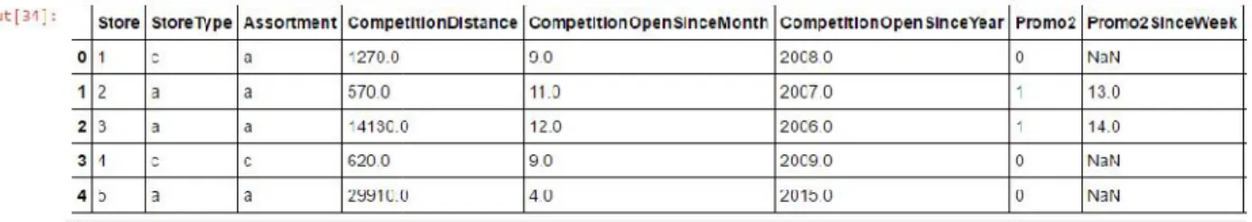
5.8 Data visualization and analysis
Store
Table 1: Store data representation
#Information of 1116 stores
Page28of45
Assortment - Describes an assortment level: a = basic, b = extra, c = extended
CompetitionDistance - Distance in meters to the nearest competitor store
CompetitionOpenSince [Month/Year] - Approximate year and month of the time the nearest competitor was opened
Promo - Indicates whether a store is running a promo on that day
Promo2 - Continuing and consecutive promotion for some stores: 0 = store is not participating
1 = store is participating
Promo2Since [Year/Week] - Describes the year and calendar week when the store started participating in Promo2
PromoInterval - Describes the consecutive intervals Promo2 is started, naming the months the promotion is started a new.
5.8 Data visualization and analysis
Store
Table 1: Store data representation
RangeIndex(start=0, stop=1115, step=1) # Total 10 attributes
Index(['Store', 'StoreType', 'Assortment', 'CompetitionDistance',
'CompetitionOpenSinceMonth', 'CompetitionOpenSinceYear', 'Promo2', 'Promo2SinceWeek', 'Promo2SinceYear', 'PromoInterval'], dtype='object')
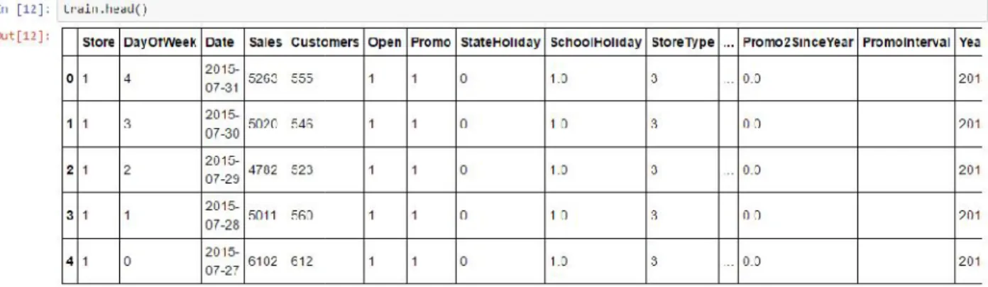
Train
Table 2: Train data representation
# Total train data is 844338
Int64Index([ 0, 1, 2, 3, 4, 5, 6, 7 , 8, 9, ...
844328, 844329, 844330, 844331, 844332, 844333, 844334, 844335 , 844336, 844337], dtype='int64', length=844338)
#Total 26 attributes
RangeIndex(start=0, stop=1115, step=1) # Total 10 attributes
Index(['Store', 'StoreType', 'Assortment', 'CompetitionDistance',
'CompetitionOpenSinceMonth', 'CompetitionOpenSinceYear', 'Promo2', 'Promo2SinceWeek', 'Promo2SinceYear', 'PromoInterval'], dtype='object')
Train
Table 2: Train data representation
# Total train data is 844338
Int64Index([ 0, 1, 2, 3, 4, 5, 6, 7 , 8, 9, ...
844328, 844329, 844330, 844331, 844332, 844333, 844334, 844335 , 844336, 844337], dtype='int64', length=844338)
Page30of45
Index(['Store', 'DayOfWeek', 'Date', 'Sales', 'Customers', 'Open', 'Promo' , 'StateHoliday', 'SchoolHoliday', 'StoreType', 'Assortment', 'CompetitionDistance',
'CompetitionOpenSinceMonth', 'CompetitionOpenSinceYear', 'Promo2',
'Promo2SinceWeek', 'Promo2SinceYear', 'PromoInterval', 'Year', 'Month', 'Day', 'WeekOfYear', 'CompetitionOpen', 'PromoOpen', 'monthStr', 'IsPromoMonth'], dtype='object')
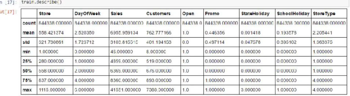
Table 3: Store data representation
We start our analysis with Table 3 that shows amount of nans and unique values if there less than 10 of them.
Page30of45
Index(['Store', 'DayOfWeek', 'Date', 'Sales', 'Customers', 'Open', 'Promo' , 'StateHoliday', 'SchoolHoliday', 'StoreType', 'Assortment', 'CompetitionDistance',
'CompetitionOpenSinceMonth', 'CompetitionOpenSinceYear', 'Promo2',
'Promo2SinceWeek', 'Promo2SinceYear', 'PromoInterval', 'Year', 'Month', 'Day', 'WeekOfYear', 'CompetitionOpen', 'PromoOpen', 'monthStr', 'IsPromoMonth'], dtype='object')
Table 3: Store data representation
We start our analysis with Table 3 that shows amount of nans and unique values if there less than 10 of them.
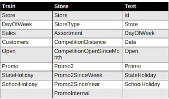
Table 4: Column by files of given Dataset Table 4: Column by files of given Dataset Table 4: Column by files of given Dataset
Page32of45 Table 5: Simple data information
Table 6: Result of Algorithms
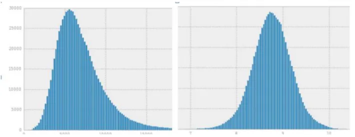
From this table we see that there are 11 NAN’s in "Open" on test also in test there only zero 'a' value in "StateHoliday" field(it'sdifferent from what we see in training set). On the next figure 1 we see distribution among all sales (left part of figure 5). I took logarithm of it and it became even more bell-shaped (right part of figure 5).
Figure 5: Distribution among all sales (left side); logarithm of it (right side)
Also from Table 4, we clearly see that we have field sales and customers that are presented in Train.csv, but not presented in Test.csv. Sales are not presented since we should predict the
Page32of45 Table 5: Simple data information
Table 6: Result of Algorithms
From this table we see that there are 11 NAN’s in "Open" on test also in test there only zero 'a' value in "StateHoliday" field(it'sdifferent from what we see in training set). On the next figure 1 we see distribution among all sales (left part of figure 5). I took logarithm of it and it became even more bell-shaped (right part of figure 5).
Figure 5: Distribution among all sales (left side); logarithm of it (right side)
Also from Table 4, we clearly see that we have field sales and customers that are presented in Train.csv, but not presented in Test.csv. Sales are not presented since we should predict the
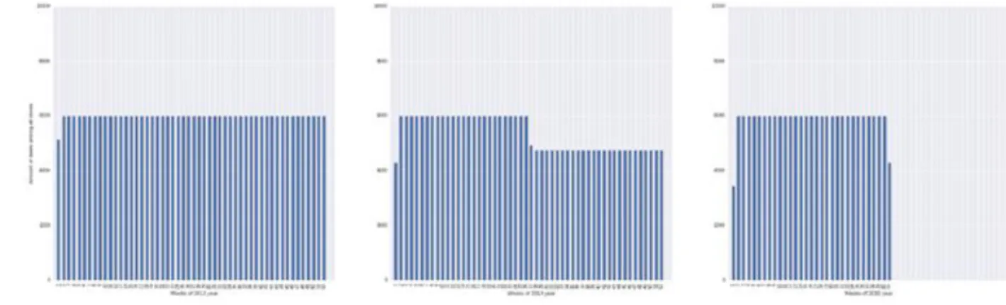
values of this field for whole this Test.csv. Customers are notpresented since they highly correlate with Sales field. We plotted graph date days in training set by week and over all stores andyears.
Figure 6: Amount of days by weeks and by years among all stores.
we see, that in the second year (2014) there is a clearly less days registered since 27-th week andamount of days restored since New Year (2015). It happens, because statistics for 180 store ids are missing since 27-th week up to 52 week but they present in test set (we should predict for them). One more point, that we found that last 5 days of month greatly changes the behavior of sales curve.
5.6 Features
A plethora of features were considered during experimentation but finally the features listed below had the greatestimpact on the model
Page34of45
1) Mean Sale per store per day of the week for a particular store Type 2) Day of the week
3) Store Type 4) Assortment
5) log (Distance from nearest competition) 6) Promo
7) Month 8) Year
9) School Holiday
The comparison of sales for a store (262) on Sunday vs the other days of the week. The graph justifies theassumption that sales on Sunday are better than the rest of the week. There is a direct correlationbetween the number of customers and the store sales. Fromthe distribution in the graph, it is very evident that the sales are much higher if the store is of type‘b’ as compared to
theother store types ‘a’, ‘c’, and ‘d’. In addition the number of customers per store over a time period is highest for store b justifying our assumption indicate that the assortment of products being sold at a store logically impacts sales as customers tend to buy items according to their needs and availability. From the distribution, it is very evident that the sales are highest if the store has an assortment level of ’a’ which implies ’extra’, followed by the assortment level ’c’
which indicates is‘extended’. The sales are least if the assortment level is ‘basic’. This inference matches with the common sense reasoning that sales increases as the assortment of products
increases and customers prefer visiting stores with greater assortment. Identifying how sales are linked to seasonal trends.
Chapter VI: Machine learning algorithms and approaches
In our work, we tried to follow Prof. Andrew Ng workflow. Unfortunately, his approach to analyze learning curve is not clearly useful because we deal with time series date and older data not always train our model better and we can say that old data isequally useful as recent one. We started with linear regression because it is a really simplest and fastest (in terms of
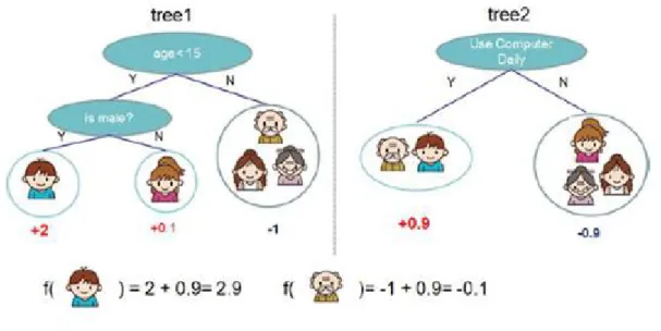
implementation time) model. We can increase number of trees to as much as we want and make it as large as we want only computational timereally matters in this case. Figure 3 perfectly describes the decision tree in case of regression problem.
Figure 7: Decision tree of xgboost library for regression problem
increases and customers prefer visiting stores with greater assortment. Identifying how sales are linked to seasonal trends.
Chapter VI: Machine learning algorithms and approaches
In our work, we tried to follow Prof. Andrew Ng workflow. Unfortunately, his approach to analyze learning curve is not clearly useful because we deal with time series date and older data not always train our model better and we can say that old data isequally useful as recent one. We started with linear regression because it is a really simplest and fastest (in terms of
implementation time) model. We can increase number of trees to as much as we want and make it as large as we want only computational timereally matters in this case. Figure 3 perfectly describes the decision tree in case of regression problem.
Page36of45
We tried to ensemble different algorithms even if we trained our models based on xgboost. The first step was to implement very simple model just to have a baseline. We split our training data set in two parts. First part is fortraining data set and second part is for test training data set. We can't truncate 70% of training set and set this as training set, and 30% as test set, since this probleminvolves time series and old data might produce non-relevant prediction. We tried very simple model as a baseline. Without any regularization, since weclearly do not over fit our data. We see that such simple model can't represent our data properly since it lack of features and what isreally meaningful that it separates space badly.
The second step that we made was to take mean of sales grouped by Store and DayOfWeek, and report that mean as a prediction. The intuition behind it, that we made more complex model with samefeatures. The learning curve is on figure 5. The greater error value means we use older data. All other learningcurves are given based on same scheme. The third step we substituted simple mean with linear regression just like in first step but now we have a lot of such linearregressions for each group separated by Store, DayOfWeek, Promo, SchoolHoliday, Open. The forth step we used extreme gradient boosting(xgboost). This is a library that is designed, and optimized
forboosted (tree) algorithms. We used these features,
Store,CompetitionDistance,CompetitionOpenSinceMonth,CompetitionOpenSinceYear,Promo,Pr omo2,Promo2SinceWeek,Promo2SinceYear,SchoolHoliday,DayOfWeek,month,year,day,year,St oreType,Assortment that gave meerror 0.125363557979. As a fifth experiment,we mixed models with different numbers of iterations (200,300,450,500) of trees
Chapter VII: Results
For the final mode, we used same configuration for all xgboost models in ensemble (except number of trees):
Params = {"objective": "reg: linear", "eta": 0.25, "max_depth": 8, "silent": 1, "subsample": 0.7, "colsample_bytree": 0.7, "seed": 1, "booster": "gbtree"} num_trees = 300.
Page38of45
We used random search tofind these parameters. In simple grid search, we go over fixed points in space and simply try our model. In grid search, we onlyspecify range in which parameters can vary and then chose points with random coordinates.
7.1 Prediction Modelling using Decision Tree
Decision tree algorithm is a very popular way to design a predictive modeling. Decision tree builds classification or regression models in the form of a tree structure. It breaks down a dataset into smaller and smaller subsets while at the same time an associated decision tree is
incrementally developed. The final result is a tree with decision nodes and leaf nodes. A decision node (e.g. Sales) has two or more branches (e.g. Holiday, Week/year). Leaf node (e.g., Result) represents a classification or decision. The topmost decision node in a tree which corresponds to the best predictor called root node. Decision trees can handle both categorical and numerical data. Decision tree built on the calculation of Entropy and Information gain.
7.2 Tools and Platforms
Anaconda is a freemium[21] open source[22] distribution of the Python and R programming languages for large-scale data processing, predictive analytics, and scientific computing, that aims to simplify package management and deployment.[23][24][25][26][27] Its package management system is conda.
7.3 Challenges
Handling large amount of sales data (10,17,210 observations on 13 variables)
Some 180 stores were closed for 6 months. Unable to fill the gap of sales for those stores.
Prediction of sales for individual stores (out of 1115) and most of stores have different pattern ofsales. A single model cannot fit to all stores.
7.4 Learnings
Exploring large datasets using visualization tools.
Learn the application of XG Boost.
7.5 Future works
Sales prediction plays a vital role in increasing the efficiency with which stores can operate as it provides details on the traffic a store can expect to receive on a given day. In addition to just
Page40of45
predicting the expected sales, there are other data which can be mined to highlight important trends and also improve planning. Briefly they are
-1) Advertisement: Identifying which customers will reactpositively to certain ad’s[15] and offers to ensure they receive them. Conversely identifying customers who do not like certain offers will help reduce sending out unnecessary offers.
2) Recommendations: Once the category of products a customer is interested in is identified, he can be recommended other products [9] he may like thereby increasing sales.
3) Predicting Demand: In addition to predicting sales, predicting the demand [11] is another solution which would immensely benefit stores. Prior knowledge of as future work, we will use external weather data and actually we tried to use it and find that difference betweentemperature of current day and previous one significantly influential on curve of number of sales. If we add features like that to our model probably we get even better score.What products will be in demand will help stores stock up on the right items.
4) Customer Based Pricing: This solution involves identifying the appropriate discounts for different items so as to maximize revenue [10]. Identifying the right product will help generate profit as well as clear excess stock.
5) Holiday / Extended Sale Planning: Involves identifying the best products to offer discounts or promos on during holidays by predicting demand. In addition finding out the best time period to offer discounts will benefit stores as well as the customers.
6) Product Classification: Classifying products into a single category will help stores offer the best products to customers. Stores can avoid stocking up on redundant products as well as those
that customers may not buy together.
7.6 CONCLUSION
In this project we have performed sales forecasting for stores using different data mining techniques. The task involved predicting the sales on any given day at any store. In order to familiarize ourselves with the task we have studied previous work in the domain including Time Series Algorithm as well as a spatial approach. A lot of analysis was performed on the data to identify patterns and outliers which would boostor impede the prediction algorithm. The features used rangedfrom store information to customer information as well associo-geographical
information. Data Mining methods like Linear Regression, Random Forest Regression and XGBoost were implemented and the results compared. XGBoost which is an improved gradient boosting algorithm was observed to perform the best at prediction. With efficiency being the way forward in most industries today, we aim to expand our solution to help stores improve
Page42of45
REFERENCES
[1] Shirley Coleman AhlemeyerStubbe, Andrea. A practical guide to data mining for business and industry.John Wiley and Sons, 2014.
[2] P. Mekala B. Srinivasan. Time series data prediction on shopping mall.In International Journal of Research in Computer Application and Robotics, Aug 2014.
[3] Gordon S. Linoff Berry, Michael JA. Data mining techniques: for marketing, sales, and customer relationship management. John Wiley and Sons, 2004.
[4] L. Breiman. Random forest. Mach. Learn., 4:5–32, 2001. [5] Tianqi Chen. Xgboost https://github.com/tqchen/xgboost.
[6] Douglas C Montgomery et all. Introduction to Linear Regression Analysis.Number 5.Wiley, 2012.
[7] Jerome H. Friedman. Stochastic gradient boosting.Computational Statistics and Data Analysis, pages 367–378, 2002.
[8] et al. Huang, Wenjie. A novel trigger model for sales prediction with data mining techniques. Data Science Journal, 14, 2015.
[9] et al. Jannach, Dietmar. Recommender systems: an introduction. Cambridge University Press, 2010.
[10] Romana J. Khan and Dipak C. Jain.An empirical analysis of price discrimination mechanisms and retailer profitability. Journal of Marketing Research, 42.4:516–524, 2005. [11] A. GürhanKök and Marshall L. Fisher. Demand estimation and assortment optimization under substitution: Methodology and application.
Operations Research, 55.6:1001–1021, 2007.
[12] M Nakanisihi LG Cooper. Market Share Analysis, 2010.
[13] Simon Scheideret. allMaike Krause-Traudes. Spatial data mining for retail sales
forecasting.11th AGILE International Conference on Geographic Information Science, 2008. [14] Andrew G Parsons. The association between daily weather and daily shopping patterns. Australasian Marketing Journal (AMJ), 9.2:78–84, 2001.
[15] Nicholas J. Radclifte and Rob Simpson. Identifying who can be saved and who will be driven away by retention activity. Journal of Telecommunications Management, 1.2, 2008. [16] Rossmann. https://www.kaggle.com/c/rossmann-store-sales.
Page44of45
[17] et al Schroeder, Glenn George. System for predicting sales lift and profit of a product based on historical sales information. U.S. Patent No. 7,689,456, 2010.
[18] A. Liawet. all V. Svetnik. Random forest: a classification and regression tool for compound classification and qsar modeling. J. Chem. Inf. Comput. Sci., 43, 2003.
[19] Wayne L. Winston. Analytics for an Online Retailer: Demand Forecasting and Price Optimization. Wiley, 2014.
[20] "Anaconda End User License Agreement". continuum.io. Continuum Analytics. Retrieved May 30, 2016.
[21] "Anaconda Subscriptions". continuum.io. Continuum Analytics. Retrieved September 30, 2015.
[22] "Open Source is at the Core of Modern Software". continuum.io. Continuum Analytics. Retrieved May 30, 2016.
[23] Martins, Luiz Felipe (November 2014). IPython Notebook Essentials (1st ed.). Packt.p. 190.ISBN 9781783988341.
[24] Gorelick, Micha; Ozsvald, Ian (September 2014). High Performance Python: Practical Performant Programming for Humans (1st ed.). O'Reilly Media.p. 370.ISBN 9781449361594. [25] Jackson, Joab (February 5, 2013). "Python gets a big data boost from DARPA". Network World.IDG.Retrieved October 30, 2014.
[26] Lorica, Ben (March 24, 2013). "Python data tools just keep getting better". O'Reilly Radar.O'Reilly Media.Retrieved October 30, 2014.
[27] Doig, Christine (February 1, 2016). "Anaconda for R users: SparkR and rBokeh". Developer Blog.Continuum Analytics.