University of Kentucky University of Kentucky
UKnowledge
UKnowledge
Theses and Dissertations--Economics Economics
2020
Three Essays on the Economics of Education Expansion
Three Essays on the Economics of Education Expansion
Xiaozhou DingUniversity of Kentucky, xiaozhou.ding@uky.edu Author ORCID Identifier:
https://orcid.org/0000-0003-2785-069X
Digital Object Identifier: https://doi.org/10.13023/etd.2020.191
Right click to open a feedback form in a new tab to let us know how this document benefits you. Right click to open a feedback form in a new tab to let us know how this document benefits you.
Recommended Citation Recommended Citation
STUDENT AGREEMENT: STUDENT AGREEMENT:
I represent that my thesis or dissertation and abstract are my original work. Proper attribution has been given to all outside sources. I understand that I am solely responsible for obtaining any needed copyright permissions. I have obtained needed written permission statement(s) from the owner(s) of each third-party copyrighted matter to be included in my work, allowing electronic distribution (if such use is not permitted by the fair use doctrine) which will be submitted to UKnowledge as Additional File.
I hereby grant to The University of Kentucky and its agents the irrevocable, non-exclusive, and royalty-free license to archive and make accessible my work in whole or in part in all forms of media, now or hereafter known. I agree that the document mentioned above may be made available immediately for worldwide access unless an embargo applies.
I retain all other ownership rights to the copyright of my work. I also retain the right to use in future works (such as articles or books) all or part of my work. I understand that I am free to register the copyright to my work.
REVIEW, APPROVAL AND ACCEPTANCE REVIEW, APPROVAL AND ACCEPTANCE
The document mentioned above has been reviewed and accepted by the student’s advisor, on behalf of the advisory committee, and by the Director of Graduate Studies (DGS), on behalf of the program; we verify that this is the final, approved version of the student’s thesis including all changes required by the advisory committee. The undersigned agree to abide by the statements above.
Xiaozhou Ding, Student Dr. Christopher Bollinger, Major Professor Dr. Josh Ederington, Director of Graduate Studies
THREE ESSAYS ON THE ECONOMICS OF EDUCATION EXPANSION
DISSERTATION
A dissertation submitted in partial fulfillment of the requirements for the
degree of Doctor of Philosophy in the Gatton College of Business and
Economics at the University of Kentucky
By Xiaozhou Ding
Lexington, KY
Co-Directors: Dr. Christopher Bollinger, Professor of Economics and Dr. Steven Lugauer, Associate Professor of Economics
2020
Copyright © Xiaozhou Ding, 2020.
ABSTRACT OF DISSERTATION
THREE ESSAYS ON THE ECONOMICS OF EDUCATION EXPANSION
My dissertation consists of three essays that study the unintended consequences of edu-cation policies. The first two essays examine the impact of higher eduedu-cation expansion in China on household saving rate and individual migration rate. The third essay looks into the impact of a school redistricting plan and the construction a new school on housing prices in Fayette County, Kentucky.
In the first essay, I utilize the large national expansion on higher education in China which exogenously increase the enrollment of college students, to estimate the induced change in the expected college probability and how it affects saving rates for households with young children both before and after the expansion. I find a ten percentage increase in the change in college probability raises household saving rates by more than seven percentage points.
In additional to analyzing the saving behaviors of households, I analyze the migration rates of young adults in China using the same policy shock. I use an instrumental variable approach and instrument college status by access to college in province-college year level to identify the effect of college attendance on young adults’ later life location choice. 2SLS estimates suggest that attending college significantly increases the likelihood of residing in a different province later in life by 9.1 percentage points.
In the third essay, I take advantage of the approval of school redistricting plan in Fayette County, Kentucky to examine the impact of school quality on housing prices. I find prices for homes redistricted from a lower-performing school into the proposed school catchment area increase by six percent. For houses in higher-performing school catchment areas redistricted to the proposed new school district, there is a smaller in-crease in value. Houses redistricted from higher-performing schools to lower-performing schools decrease in value by three to five percent. The estimate shows that homes in the redistricted areas increased by $108 million relative to homes that were not redistricted.
KEYWORDS: College Expansion; China; Saving Rate; Migration; School Quality; Hous-ing Prices
Author’s signature: Xiaozhou Ding
THREE ESSAYS ON THE ECONOMICS OF EDUCATION EXPANSION
By Xiaozhou Ding
Co-Director of Dissertation: Dr. Christopher Bollinger
Co-Director of Dissertation: Dr. Steven Lugauer
Director of Graduate Studies: Dr. Josh Ederington
ACKNOWLEDGMENTS
First, I would like to thank my entire family. I thank my parents, Jiakui Ding and Ying Lin, for their countless support throughout my entire life and constant encouragement in the years I pursued my education. They taught me to keep my integrity and to have a good work ethic all the time, which walked me through all the difficult times. Most of all, I thank my wife, Yaxiang Song, whose unshakable love and patience accompanied me during the years that I was in pursuit of my doctoral degree and continue to do so today. I would like to thank my co-advisor, Christopher Bollinger, for the dedicated guid-ance he has provided since I entered the graduate program five years ago. His humor and straightforwardness helped me survive all stages of boring regressions and challenging presentations. But most importantly, he instilled in me a passion for economics and care-ful research. I also thank my co-advisor, Steven Lugauer. I am gratecare-ful for the continued support and encouragement from the moment I entered his office. Always paying atten-tion to the details is one of the most important things I learned from my countless hours of discussions with him during my work on this dissertation.
Also, I would like to thank my committee member and the department chair William Hoyt, for his tremendous support and inspiring comments regarding my research. With-out his support, this dissertation would not have been possible. I also thank him for the numerous weekends I saw him working in his office, which motivated me to work harder and harder. I thank Michael Samers for his valuable comments that pushed me to think harder on the broader picture of my research. I also appreciate the time and input of the outside examiner, Brian Bratten.
Thank you to Jenny Minier, for her encouragement and willingness to seek out sugges-tions from graduate students when considering improvements to the program. I am also grateful to Lala Ma for her support and help to start publishing journal articles. This disser-tation has also benefited greatly from the feedback of several members of the Department of Economics including, but not limited to, Ana Herrera, Carlos Lamarche, Frank Scott, Ken Troske, Josh Ederington, Anthony Creane, Aaron Yelowitz, Alejandro Dellachiesa, Darshak Patel, James Ziliak, Charles Courtemanche, David Agrawal, and Olga Malkova. I also appreciate the continued support from Michael Childress, Bethany Paris, and Michael Clark at the Center for Business and Economic Research.
nides, Jeffrey Zabel, David Garman, and Steven Block at Tufts University. I thank Guang-ping Zhu, Xiaohua Shi, Xueling Zhou, Mingming Mei, JianGuang-ping Hu, LuGuang-ping Li, Rong Liu, Fuzhong Hong, and others who contributed to various other stages of my education.
I am grateful to the constant support from Real Limoges, Xingya Luo, Weifeng Zhou, Congchi Zhang, Qishu Shen, Yao Wu, Xinyue Hua, Yinglei Xu, Yu Cao, Kun Yu, and my roommates and friends from class one of finance at Chongqing Technology and Busi-ness University. Their deep understanding and endless support provided faith and fun throughout my studies.
Without my family, my advisors, the faculty, my friends, and all others at various sem-inars, conferences, and meetings who have provided me with discussions and comments this dissertation would not have been possible, so thank you.
TABLE OF CONTENTS
Acknowledgments . . . iii
Table of Contents . . . v
List of Tables . . . viii
List of Figures . . . ix
Chapter 1 Introduction . . . 1
Chapter 2 The Expansion of Higher Education and Household Saving in China . . 3
2.1 Introduction . . . 3
2.2 Saving and Higher Education in China . . . 6
2.2.1 Household Saving Rates in China . . . 6
2.2.2 Background on Higher Education Enrollment Policy . . . 8
2.3 A Model of Households Saving for College . . . 9
2.4 Data . . . 12
2.5 Empirical Approach . . . 14
2.6 Higher Education Expansion’s Effect on Saving. . . 16
2.6.1 Who Goes to College? . . . 16
2.6.2 The Main Empirical Findings . . . 17
2.7 Other Explanations for China’s High Saving Rates . . . 19
2.7.1 Other Reforms . . . 20
2.7.2 Household Demographics . . . 21
2.8 Conclusion . . . 23
2.9 Tables . . . 24
2.10 Figures . . . 29
Chapter 3 College Education and Internal Migration in China . . . 35
3.1 Introduction . . . 35
3.2 Motivation and Related Literature . . . 38
3.3 Internal Migration and Higher Education in China . . . 40
3.4 Model . . . 41
3.7.2 Robustness Checks . . . 48
3.8 Discussion . . . 49
3.8.1 Hukou Restriction. . . 49
3.8.2 College Expansion . . . 52
3.8.3 Beliefs in Family Network, Social Connections, and Education . . . 53
3.8.4 Placebo Tests . . . 55
3.9 Conclusion . . . 55
3.10 Tables . . . 57
3.11 Figures . . . 67
Chapter 4 How Do School District Boundary Changes and New School Proposals Affect Housing Prices . . . 71
4.1 Introduction . . . 71
4.2 Literature Review . . . 73
4.3 The Impacts of Rezoning School Boundaries on Property Values . . . 76
4.3.1 An Open City Model . . . 76
4.4 Background of Redistricting in Fayette County . . . 78
4.5 Empirical Strategy and Data . . . 80
4.5.1 Difference-in-Differences . . . 80
4.5.2 Data and Summary Statistics . . . 82
4.6 Results . . . 84
4.6.1 Unconditional Switching Effect . . . 84
4.6.2 Test Scores Effect . . . 85
4.6.3 Disaggregating the Impacts of Redistricting . . . 87
4.6.4 Who Benefits from the Boundary Change? . . . 89
4.7 Extensions and Tests of the Model . . . 90
4.7.1 Information Updating . . . 90 4.7.2 Placebo Test . . . 92 4.8 Conclusion . . . 92 4.9 Tables . . . 94 4.10 Figures . . . 105 Chapter 5 Conclusion . . . 109 Appendix . . . 112
Appendix A: Structural Model for Chapter 2 . . . 112
Derivation of Proposition 1 . . . 112
Saving Response for High-Saving Households . . . 114
Appendix B: Data and Variable Definition for Chapter 2 . . . 115
Appendix C: Addition Tables for Chapter 2 . . . 115
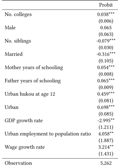
Probit Estimates . . . 115
Triple Difference-in-Difference Estimates . . . 117
Appendix D: Data for Chapter 3 . . . 120
CFPS Data . . . 120
Higher Education Expansion . . . 123
Hukou Reform Data . . . 124
Appendix E: Additional Tables for Chapter 3 . . . 126
References . . . 128
Vita . . . 139
Education . . . 139
Employment . . . 139
Peer-Reviewed Publications . . . 139
LIST OF TABLES
2.1 Summary Statistics by Year and Children’s Age . . . 24
2.2 College Probability’s Effect on Household Saving Rates . . . 25
2.3 Robustness Checks. . . 26
2.4 Changes in the Relative Savings on Initial Low and High Savers . . . 26
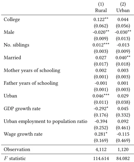
2.5 Other Reforms . . . 27 2.6 Demographics . . . 28 3.1 Summary Statistics . . . 57 3.2 Probit Result . . . 58 3.3 Main Result . . . 59 3.4 Robustness Check . . . 60
3.5 Impact of College on Cross-Province Migration for Different Childhood hukou Status . . . 61
3.6 In- and Out-Birth Hukou Province Migration . . . 62
3.7 The Differential Impact of College Education on Migration before and after Expansion . . . 63
3.8 Decomposition of Changes in Migration Probability . . . 64
3.9 IV Results of College Education on Personal Beliefs . . . 65
3.10 Placebo Tests . . . 66
4.1 Number of Sales based on the Rezoned School Districts, 2003-2017 . . . 94
4.2 Summary Statistics . . . 95
4.3 Main Results . . . 96
4.4 Boundary Fixed Effect . . . 97
4.5 Log of Sale Price on ACT Scores, Pre- and Post-Catchment Area Changes . . . 98
4.6 LN(Sales Price) on Pre- and Post-Announcement Catchment Area Changes by Catchment Change . . . 99
4.7 Housing Stock Value Change . . . 100
4.8 LN(Sales Price) on Pre- and Post-Announcement Catchment Area Changes and Catchment Change×Number of Fullbaths . . . 101
4.9 LN(Sales Price) on Pre- and Post-Announcement Catchment Area Changes and Catchment Change×LN(Square Footage) . . . 102
4.10 Information Updating . . . 103
4.11 Placebo Test . . . 104
LIST OF FIGURES
2.1 Household Saving Rates . . . 29
2.2 China Higher Education Expansion . . . 29
2.3 New Students Enrolled and the Enrollment Rate . . . 30
2.4 Cost of Education . . . 31
2.5 Enrollment Rate by Province . . . 32
2.6 Estimated College Probability for 2002 Households . . . 33
2.7 Saving Rate and Change of Probability for 2002 Households. . . 34
2.8 Test for Pre-Trends . . . 34
3.1 China’s Migration Population, 1982-2017 . . . 67
3.2 Number of Colleges . . . 67
3.3 Variation in Number of Colleges . . . 68
3.4 Pre-Trend Test of Migration Rate Change and Number of Colleges Change . . 68
3.5 Number of Colleges and Hukou Reform . . . 69
3.6 The Geography of Cross-Province Migration . . . 69
3.7 Share of College People by Rural/Urban hukou at Age 12 . . . 70
4.1 Old School Catchment Boundary . . . 105
4.2 New School Catchment Boundary . . . 105
4.3 Change in High School Catchment Area Boundaries . . . 106
4.4 Median House Price by High School Catchment Area and Year . . . 107
4.5 Composite ACT Score by High School and Year. . . 107
4.6 Sales Price Trends for Treatment Group (Houses subject to Redistricting) and Control Group (Houses not subject to Redistricting . . . 108
Chapter 1 Introduction
Policies related to education are important in every country because they affect human
capital accumulation which has a long-term effect that pass on generations and promote
economic growth. Moreover, such policies could lead to indirect consequences that impact
household financial behaviors, individual migration decisions, and housing prices. My
dissertation consists of three essays that study the unanticipated impacts of policies that
change the supply side of education. The first two essays examine the unintended
conse-quences of college expansion in China on household saving and individual cross-province
lifetime migration. The third essay looks at how school redistricting and construction of
a new school affect housing prices in Fayette County, Kentucky.
In the first essay, I study whether access to higher education impacts household
sav-ing behavior ussav-ing survey data from Chinese households dursav-ing a time of unprecedented
higher education expansion. I begin by estimating the change in the expected probability
of college admittance for each family with young children following the education
expan-sion. Then I estimate how the increase in college probability affected household saving
rates by comparing households before and after the reform. The results indicate that a
10-percentage point increase in the probability of going to college raises the saving rate
for a household with school-age children by more than 7 percentage points.
The second essay examines the causal impact of college education on young adults
cross-province migration in China using China Family Panel Studies 2010 wave data. In 1999 China implemented higher education expansion which caused rapid increase in
num-ber of colleges for every province. I take advantage of such shock and instrument college
status by access to college in province-college-year level to identify the effect of college
attendance on young adults’ later life location choice. 2SLS estimates suggest that
attend-ing college significantly increases the likelihood of residattend-ing in a different province later
in life by 9.1 percentage points. The results are robust to a set of specifications and tests.
The third essay uses changes in school boundaries and the proposal of a new school
in Fayette County, Kentucky to estimate the value of schools through capitalization in
home prices. The findings from redistricting in the Fayette county school district show that prices for homes redistricted from a lower-performing (based on test scores) school
into the proposed school catchment area increase by six percent. For houses in
higher-performing school catchment areas redistricted to the proposed new school district, there
is a smaller increase in value. Houses redistricted from higher-performing schools to
lower-performing schools decrease in value by three to five percent. However, many of
the redistricted properties see little or no significant change, suggesting that only extreme changes in school quality are capitalized. I estimate that homes in the redistricted areas
Chapter 2 The Expansion of Higher Education and Household Saving in China
2.1 Introduction
China’s household saving rate has increased dramatically since economic reforms began
in 1978. Before the reforms, households typically saved less than five percent of their
in-come. Saving gradually trended up during the 1980s and 1990s, before rapidly accelerating
after 2000. Now, households save over twenty-five percent of their income, on average.
The saving has helped maintain a high investment rate within China and allowed funds to
flow abroad, particularly to the United States. Several theories have been put forward to explain the high saving rates, including demographic changes (Modigliani and Cao,2004;
Curtis, Lugauer, and Mark, 2015; Imrohoroglu and Zhao, 2018b; Ge, Yang, and Zhang,
2018), income uncertainty (Chamon, Liu, and Prasad, 2013), private expenditures (
Cha-mon and Prasad,2010), economic reforms (He et al.,2018), and gender-related issues (Wei
and Zhang, 2011; Zhou, 2014). None of the theories fully explains the changes. In this
chapter, I provide evidence that household saving responds strongly to the expansion of
college opportunities.
Entrance into higher education in China is determined by an exam and quotas set by
the Ministry of Education. In 1999, the Ministry of Education began an extensive increase in the number of students allowed to enroll in college. The enrollment rate for high-school
graduates quickly moved from approximately twenty percent to almost sixty percent, and
is now eighty percent. China currently has almost forty million college students, about
one-fifth of the college students in the world. This unprecedented education expansion
likely impacts society in a number of ways. One of the most obvious effects, and the
fo-cus of this paper, is that Chinese households must finance their child’s education. Since
student loans were not common in China in the early years of the higher education
ex-pansion (Shen and Li,2003), households paid for tuition out of accumulated savings or
current income. My hypothesis is that as enrollment rates increased, households with young children saved more in anticipation of future education related expenses.
Understanding the link between saving and education is important for many reasons.
First, understanding saving behavior itself is, of course, important, and education
ex-penses are a key part of household expenditures, over 10 percent on average in China.
Second, researchers and policy makers are interested in explaining China’s high saving
rate in particular because, as mentioned, Chinese savings are a major component of
inter-national capital flows. China owns a large portion of European and US debt. The saving
has also helped to fuel China’s dramatic economic growth. Third, the relationship between saving and education may be informative for public policies of human capital
accumula-tion. Many countries are debating whether to increase access to higher education, and it
is natural to question how the additional schooling will be financed. Research is needed
on how the expansion of education affects the economy and how households respond to
the increase in college opportunities. I find that affected households sharply increase their
saving.
To motivate my empirical approach and to clearly articulate the connection between
education expansion and saving, I first present a simple two-period theoretical model of
household saving. In the model, households receive income only in period 1 and must save for period 2. Households also can save to pay for college. If a household saves enough to
pay tuition and expenses, and their child gets admitted, then the household reaps the
ben-efits of having a college graduate. If a household does not save enough, their child cannot
attend college. Thus, households compare the utility obtained from consuming more in
period 1 against the expected utility from possibly sending their child to college and
hav-ing greater consumption in period 2. As the expansion of higher education increases the
probability of acceptance into college, the expected utility of saving for college increases.
If the expected utility of saving for college becomes larger than that of not doing so, then
the household increases their saving rate in order to have enough to pay for college. Thus,
the model suggests that household saving rates should go up for households experiencing a large increase in the likelihood of sending their children to college.
Based on this intuition, I take China’s 1999 higher-education expansion as a
natu-ral experiment and estimate how the policy-induced changes in the likelihood of college
affected saving rates. My empirical strategy consists of two steps. The first step is to
cal-culate the change in the expected probability of college for individual households. To do
this, I estimate a probit model for the probability of children’s college status using
cross-sectional household level information from the 1995 and 2002 China Household Income
Project (CHIP) surveys. The data allows me to see whether a family has children, their
ages, and whether the children attend college. I estimate the probit model separately for each year using a host of control variables and only the subset of families with
college-tend college in the future. While college opportunities increased for almost all groups, the increase was highest for wealthy households with low levels of (parental) education from
certain provinces. I assume that the policy (which induced the changes in college
prob-ability) was exogenous relative to household saving rates, and I provide province-level
evidence in favor of this assumption.
In the second step of my empirical strategy, I estimate how the changes in college
probability relate to household saving rates via a quasi difference-in-differences
frame-work. Specifically, I regress household saving rates on a set of covariates and the
esti-mated change of college probability (separately) for both households in the 1995 survey
and 2002 survey. I include province fixed effects and allow all the parameter estimates (on the fixed effects and other controls) to differ between the 1995 and 2002 regressions to
allow for variation in the observables’ effects. I interpret the difference between the
esti-mated coefficients on the change in college probability between the two years as the
pol-icy’s impact on saving rates. I subtract the estimated coefficient estimate generated using
the 1995 sample (before the policy was implemented) from the 2002 coefficient estimate
in order to net out any time-invariant unobservables related to the intensity of treatment
(i.e. the change in college probability). Given that the regressions include many controls,
it is difficult to think what these unobservables might be. Nevertheless, the
difference-in-differences approach helps to mitigate concerns over such omitted variables.
Consistent with the theoretical model, my main finding is that the change in the ex-pected probability of college status has a quantitatively large and statistically significant
effect on household saving rates. A 10 percentage point increase in the college
probabil-ity increases the average household’s saving rate by 7.5 percentage points. This result
provides evidence that the education expansion increased saving for households with
school-age children. My results appear to be driven by households experiencing a large
increase in the possibility of college, while households that already had ample savings do
not increase their saving rates; both these findings are also consistent with the theoretical
model.
I report on a number of alternative specifications, and my main findings remain quali-tatively unchanged. The robustness checks include omitting the provinces with the largest
changes in enrollment rates and using wealth in place of savings. I also carefully consider
other policy changes that occurred in China, including housing reform, public healthcare
reform, and the reorganization of State-Owned Enterprises. Finally, I consider some of
the large demographic changes that have been on-going in China, as previous literature
has shown that demographic factors have impacted household saving in China. I discuss
the burgeoning literature seeking to explain China’s high household saving rate in the
next section.
In addition to the recent research on China’s high saving rates, my paper also is related
to the literature on higher education expansion. For example,Che and Zhang(2018) use
an approach similar to this paper to show that the Chinese college expansion increased
human capital and improved productivity. Feng and Xia(2018) examine how the college
expansion affected technology adoption in Chinese firms. Also, see Li and Xing(2010),
Knight, Deng, and Li (2017), Li et al. (2017), and Bollinger and Hu (2017, 2018). These
papers primarily focus on labor market implications, while I connect college expansion to
saving behavior. Finally, my paper contributes to the growing literature that studies how
decisions made within the family impact the macro-economy. See Doepke and Tertilt (2016), Doepke and Zilibotti (2019), and Greenwood, Guner, and Vandenbroucke (2017)
and the many recent papers cited within for more on this growing sub-field.
The rest of this chapter is organized as follows. Section3.3documents the high saving rates among Chinese households and provides background on the education expansion.
Section3.4presents the model of household saving that motivates the empirical analysis. Section3.5introduces the data, and Section3.6discusses the estimation strategy. Section
3.7presents the main empirical findings. Section3.7.2contains additional analysis, and Section3.9concludes.
2.2 Saving and Higher Education in China
I am interested in how the expansion of higher education affects household saving
deci-sions. In this section, I document the large increase in Chinese household saving rates over
time and provide background on the relevant changes to education policy. The remainder
of the paper links these two phenomena, both theoretically and empirically.
2.2.1 Household Saving Rates in China
Throughout the paper, I define the household saving rate as
Saving rate = Income−Expenditure Income = 1− Expenditure Income . (2.1)
contributed to the high investment rate (and therefore growth rate) in China. The ex-cess saving has been flowing abroad, especially to the US and Europe. Therefore, there is
wide-spread interest in understanding why Chinese households save so much.
Several theories have been put forward. One strand of the literature has focused on
the economic reforms that have been ongoing since 1978.Chamon, Liu, and Prasad(2013)
argue that the reforms have led to uncertainty over income, pensions, and healthcare,
inducing Chinese households to save more for precautionary reasons.1 As an example of
this,He et al.(2018) show that the reform of state-owned enterprises in the 1990s increased
unemployment and other risks for Chinese households, generating a dramatic increase in
saving. Similarly,Choi, Lugauer, and Mark(2017) show that high income growth coupled with high income uncertainty helps to explain why Chinese households currently save so
much more than US households. Other papers, includingSong and Yang(2010),Lugauer
and Mark(2013),Song et al.(2015), andCurtis(2016), have studied the interaction between
saving and aggregate growth within the context of China.
A second strand of the literature has focused on the implications of China’s fertility
policies.Modigliani and Cao(2004) andCurtis, Lugauer, and Mark(2015) appeal to the
life-cycle hypothesis of household saving to argue that the large demographic changes, caused
in part by the One Child Policy, have increased saving rates over time.2 Several papers
have documented specific examples of how demographics impact saving in China.
Imro-horoglu and Zhao(2018a) argue that increases in expected old-age health costs and the aging population act together to increase savings. Rosenzweig and Zhang(2014) present
evidence showing that the increase in the prevalence of co-residing elderly parents helps
to explain household saving behavior. Wei and Zhang(2011) andZhou(2014) show that a
gender imbalance in the sex-ratio has interacted with life-cycle considerations to impact
saving.
My paper is related to these previous studies, in that the cost for higher education
has shifted to families and saving for college varies over the life-cycle.3 China radically
and very rapidly altered its higher-education policies, which allows me to study
house-holds that experienced a sudden change in their expectations for sending their children to college. I next provide background on these policy changes.
1
SeeChamon and Prasad (2010) for more on how the burden for many expenditures shifted away from collectives and onto households. Also, seeYoo and Giles(2007).
2
Also, seeBairoliya, Miller, and Saxena(2018),Banerjee et al.(2015),Chao et al.(2011),Choukhmane, Coeur-dacier, and Jin(2017),Curtis, Lugauer, and Mark(2017), andLugauer, Ni, and Yin(2017).
3
In a paper related to mine,Chen and Yang(2012) use the education reform in China to test the theory of precautionary saving. Also, note that housing in China shares these characteristics; seeChen, Yang, and Zhong(2016).
2.2.2 Background on Higher Education Enrollment Policy
College admission in China is based purely on the Gaokao (college entrance exam)
admin-istered every year in June. Students are admitted on a provincial basis, and the Ministry of
Education decides the number of students from each province. The enrollment rates vary
substantially across provinces. So, students compete for admission with other applicants
within their province. If a high school graduate fails to get into a college, they can retake
the exam and reapply in the following year. Due to the Cultural Revolution, the entrance exam was suspended between 1968 and 1978. In 1978, China initiated sweeping economic
reforms, including reinstating the college entrance exam and enrolling new students into
universities.
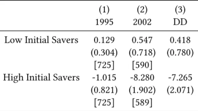
Figure 2.2 shows the number of students matriculating, total number enrolled, the number of college teachers and staff, and the number of higher institutions by year. There
were over 400,000 new students enrolled in 1978, and about 850,000 students total. The
number of students gradually increased until 1999. Then, China instituted the higher
edu-cation expansion, and enrollment exploded. In 1999 alone, the number of newly enrolled
students increased by more than 40 percent. Over 1.5 million high school students began college in 1999, and by 2012 nearly 7 million students were starting college each year.
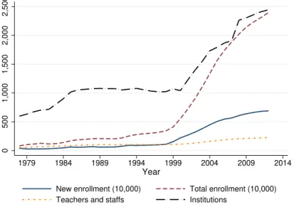
Figure2.3plots this unprecedented increase in college enrollment alongside the national enrollment rate. The jump in the enrollment rate after 1999 (from below 40 percent to
over 60) is readily apparent. My analysis focuses on this sudden policy change.
The central Chinese government designed and controlled the 1999 higher education
expansion, and it reflected the government’s political objectives. China had experienced
various social and economic headwinds in the 1990s, including a sizable reduction in
em-ployment at State-Owned Enterprises. The children of the large Chinese baby-boom
gen-eration were facing a bleak employment outlook, and the government was urged to find a solution.4 According to lore, Min Tang, an economist at the Asian Development Bank in
China, proposed enrollment expansion in a November 1998 letter to Premier Zhu Rongji.
The hope was that doubling college enrollment within three years would stimulate
invest-ment in services, construction, and other related industries and would ultimately increase
as by other observable household characteristics. I exploit the massive policy change to estimate how the expansion in higher education affected household saving.
The link between education and saving that I propose is a simple one. Households
had to save in order to afford college tuition and expenses. Student loans were not readily
available (Wang et al., 2014), and while the prevalence of college increased, so did the
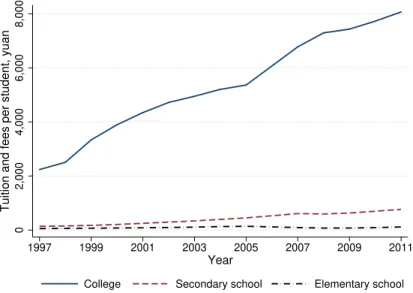
cost.5 Figure2.4plots the total annual tuition and fees per student for different types of education over time. Due to compulsory education laws, the cost of attending elementary
school and middle school remained close to zero. In contrast, the already high tuition
and fees for college went up by a factor of four. Education was (and remains) a major
expenditure category for Chinese households (Chamon and Prasad, 2010). According to Yao et al.(2011), most Chinese households save for education motives, andWei and Zhang
(2011) show that 76 percent of single-female-child households save for education.
The college expansion reform implemented by the Ministry of Education of China
serves as a good natural experiment for analyzing the impact of education expansion
on household saving. First and foremost it was a large exogenous shock. Second, the
magnitude of the expansion varied by province even though it was implemented
nation-wide. Each province received a different “quota” to determine how many students were to
be admitted, and families could not easily relocate due to the Hukou registration system.
Thus, the change in the expected probability of attending college depended on geography;
however, as I show below, other household characteristics mattered, as well. My empirical strategy leverages the exogenous variation in expected enrollment rates at the household
level. Before detailing the approach for analyzing the data, I next present a theory for
why an expansion in higher education relates to household saving behavior.
2.3 A Model of Households Saving for College
This section contains a simple two-period model of household saving decisions. My goal
is to motivate my empirical analysis by presenting an explicit theory showing how
en-rollment rates can impact saving decisions. The key choice by households in the model is whether or not to save enough to cover college tuition and expenses. An expansion in
college opportunities induces some families to increase their savings.
For tractability, I consider households with log utility over consumptionC in period 5
Credit constraints often bind even when loans can be obtained by some. SeeKeane and Wolpin(2001), Cameron and Taber(2004),Carniero and Heckman(2009),Brown, Karl Scholz, and Seshadri(2012),Sun and Yannelis(2016) andMalkova and Braga(2018) for example.
1 and expected consumptionC0in period 2.
U = lnC+ E[lnC0]. (2.2)
The household receives incomeY in period 1, which is split between consumption and savingS. Thus, the budget constraint in the first period is
C+S =Y, (2.3)
where households begin life with no assets and saving must be positive. I abstract from
discounting future utility and set the return on saving to zero, as these considerations do
not materially alter the analysis.
The household saves in order to consume in period 2, but also to potentially pay college
tuition for their child. The saving decision is made before knowing whether or not their
child will be admitted into college. However, the household does know the probability
p that their child gets in. Within the model, I interpret the education expansion as an increase inp. When a child is accepted into college, the household can pay tuition and expensesτ out of savings. If the household has not saved enough,S < τ, then the child cannot attend college. The household’s second period budget constraint is
C0 =S+Ic(θ−τ), (2.4)
whereθis the benefit from sending a child to college andIcequals one if the child attends college and zero otherwise.
I assume that the benefits of sending a child to college outweigh the costs; thus, θ >
τ > 0, and if S ≥ τ, an admitted child always enrolls in college. There are many other
ways to model the benefits from college, but this modeling choice is tractable and easy
to interpret. The household must decide whether it wants to consume less in period 1
in order to have enough saved up to potentially pay college tuition τ. The benefit θcan be taken literally as the incremental increase in old-age support from having a
college-educated child, but also more broadly to include non-monetary benefits.
With this set-up, I can examine how household saving decisions change in response to
savingτ (and possibly sending their child to college) and continuing to save less thanτ is given by the following proposition.
Proposition 1(Thresholdp). For a household choosing to save less thanτ whenp= 0, the expected utility from savingτ and saving less thanτ become exactly equal atpt>0, where the thresholdptis given by:
pt =
lnh4(YY−2τ)τi lnθτ .
(2.5)
Proposition 1 has several implications.6 Most relevantly, as higher education is
ex-panded (pincreases), a low-saving household (saving less thanτ) will start savingτ once
preaches the threshold pt. This theoretical result helps to motivate my main empirical strategy. Households experiencing a large increasep are particularly likely to increase their saving to pay for tuition. I make use of this intuition by estimating the idiosyn-cratic increases inpacross households and quantifying how changes inpimpact saving. Proposition 1 also indicates that the thresholdptdecreases with the benefits derived from collegeθ, increases with college costsτ, and decreases with income Y over the relevant range of variable values. See the Appendix for more details.
Not all households react to the increase in p in the same way, though. Households experiencing a smaller increase in p may not hit their threshold, leaving their saving behavior unchanged. Another set of households may have been saving enough to send
their children to college, S ≥ τ, prior to the education expansion. These high-saving households might have higher incomes or expected benefits from college, or they may have already faced apthat exceeded their threshold. High-saving households could even reduce their saving (but only as low asτ) aspgoes up. I show this for the model in the Appendix (and for the data in Section 2.6.2), and the result is intuitive. An increase in
pfor a household already saving more than τ merely increases the chance of obtaining
θ in period 2. This increase in expected income in period 2 lets the household consume more (and save less) in period 1, to smooth consumption. The increase in p may also reduce uncertainty, which again lowers saving. Clearly, households with older children
or no children might also react differently. The model could be expanded to consider these
additional household types; however, the remainder of the paper focuses on households with young children. I do briefly return to the issue of heterogeneous responses below,
but for the most part the exploration of different household types lies beyond the scope
of this paper.
6
I derive Proposition 1 in Section A of the Online Appendix in a straightforward way. I find the threshold
pby equating the lifetime utilities from either saving for college or not.
I introduce the data next and then provide the details of the identification strategy.
2.4 Data
I use household level information from the China Household Income Project (CHIP).7
The CHIP consists of repeated cross-sections of data from household surveys that were
conducted in five waves across 12 provinces. It is the most widely-used micro data set
on Chinese households. The survey contains questions on income and expenditures, as
well as other household characteristics such as geographic location, number of children,
and educational attainment. I use the 1995 and 2002 waves of urban households, which bracket the 1999 college expansion.
The raw data contains 6,929 household observations in 1995 and 6,835 in 2002. I focus
on households with school-age children, but I also make use of households with
college-age children. I define school-college-age as between 6 and 18 because it covers the usual
elemen-tary through high school years. I define college age as between 18 and 23, and consider
all households containing any college-age child as a college household. Households with
children between 6 and 18 (but none between 18 and 23) count as school-age children
households. I do not use households in which all children are older than 23 or younger
than 6. To hone in on prime-age workers, I drop households whose head’s age is less than
25 or above 60.
The key variable of interest is the saving rate, as calculated for each household using
Equation (2.1). To eliminate outliers, I drop households in the tails (highest and lowest one percent) of the saving rate distribution in each year. I also drop the few households that
changed Hukou after the expansion but before their children took the college entrance
exam. Lastly, I drop households from the 2002 sample in which a child took the exam
be-fore 1999 (when the expansion began) because I will use the households with college-age
children to estimate the change in the likelihood of college enrollment (due to the policy).
The final data set consists of 2,900 school-age children households and 1,218 college-age
households in 1995 and 2,357 school-age children households and 973 college-age house-holds in 2002.
chil-the large standard deviations attest, chil-there is ample variation in saving across households to exploit. In the remainder of the paper, I link the saving behavior to the expansion of
higher education. Note, that over the same time period, the average saving rate among
households with college-age children actually decreased. I do not directly study this
de-crease, but it might be related to the larger share of college-age children attending college
in 2002 (18.3 percent) versus 1995 (10.1 percent). I use this observed increase in college
attendance to estimate the changes in the expectation of attending college for younger
children.
The remainder of Table2.1reports the means and standard deviations for the control variables that I include in my regressions.8 Many of the controls also had large changes over time. For example, China’s rapid growth pushed up incomes, assets, and expenses.
Other changes can be traced to specific policies. The decreasing number of children was
likely due to fertility policies set in the 1970s. While changes in home ownership and
employment at State-Owned Enterprises (SOEs) can be traced to privatization policies
enacted in the late 1990s (Chen, Yang, and Zhong,2016; Berkowitz, Ma, and Nishioka,
2017;Chen and Wen,2017). Importantly, I not only control for variables related to these
other policy initiatives, but I also allow their impact on saving rates to vary over time.
I also run several additional robustness checks to show that these other policies do not
drive my results.
As mentioned, I use the sample of households with college-age children to estimate the change in college probability. However, since quotas for college admittance were set
at the province level, I also use province specific information on enrollment rates. For
each year and province, I approximate the enrollment rate with the ratio of new college
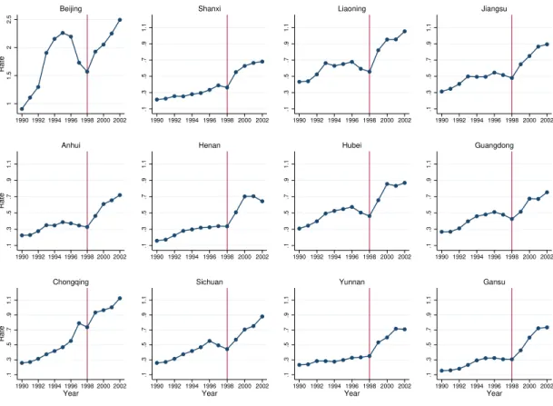
students to the number of senior high school graduates.9 Figure2.5shows the estimated college enrollment rates from the 12 provinces represented in the dataset from 1990 to
2002. In general, there is an upward trend, although many provinces dip just prior to
the expansion. After 1998, enrollment rates increase for all provinces. But neither the
enrollment rate levels nor the changes in enrollment rates are uniform across provinces.
These differences in enrollment changes were driven by policy, and they therefore help us to identify the impact on savings. The next section provides further details.
8
Appendix B provides definitions for each variable. 9
As far as I know, publicly available data on provincial college admission rates does not exist. Fan et al. (2017) uses university-specific cutoff scores collected from newspapers and websites to examine college expansion in China, andBollinger and Hu(2017) use the number of people taking the college entrance exam and subsequent enrollment at the national level.
2.5 Empirical Approach
The theoretical model in Section 3.4emitted a straightforward relationship between the policy-induced change in a household’s expectation of college and its saving rate.
How-ever, the available data (comprised of repeated cross-sections) does not track the same
households over time, and it does not contain a measure of the expected probability of
attending college. My empirical approach overcomes the data limitations in two ways.
First, I use the provincial enrollment rates in conjunction with the sample of households
with college-age children to estimate the change in college probabilities for households with younger children. Second, I use a quasi “difference-in-differences” regression
ap-proach to compare how the estimated changes in college probability affected saving rates
for households in 2002 (who were all impacted by the policy) versus how the
probabil-ity changes affected 1995 households (before the education expansion occurred). Thus,
I can net out unobserved factors that may cause a spurious relationship between saving
rates and the increased likelihood of college, leaving only the impact attributable to the
education expansion.
Specifically, I estimate Equation (2.6) twice; once using the 1995 sample of households with school-age children and once using the 2002 sample of households with school-age children.
SRij =π∆pij +Xij0 δ+λj+uij. (2.6)
The dependent variable is the saving rate (SRij) for householdifrom provincej. The coefficient (π) on the change in college probabilities (∆p) is the key parameter of interest. We obtain two estimates, one for 1995 (prior to the policy change) and one for 2002 (after
the expansion). In each separate regression,πmeasures how much of a difference having a higher∆pmakes for saving. The difference between the two estimates,π2002 −π1995, then, is akin to a differences-in-differences estimate, with the difference attributable to
the education expansion. Another interpretation is that the estimate ofπ using the 1995 households provides a “counterfactual” for what would have happened to saving rates for
Recall, for example, that the housing market changed during the late 1990s. The regres-sions allow the relationship between home ownership and savings to change, accordingly.
I return to housing (and other) reforms in Section2.7.1.
I do not directly observe ∆pij; I estimate it in two steps using the households with college-age children and the estimates of province enrollment rates described above. First,
I estimate Equation (2.7) two times, once using households with college-age children in the 1995 sample and separately using the 2002 college-age households.
pij =Xij0 β+γERi+ζj +vij. (2.7)
The dependent variable (pij) equals one if the household’s college-age child is enrolled in college, and zero otherwise. The share of college-age children attending college jumps
from about 10 percent in 1995 to over 18 percent in 2002; see Table2.1. The control vari-ables are the same as above, andζrepresents a full set of province fixed effects. Note that ERi is the household specific enrollment rate corresponding to the year that the
house-hold’s child took the college entrance exam in provincej.
With estimates of β, γ, and ζ from both 1995 and 2002 in hand, the second step is to calculate the predicted probability of college enrollment, p, for each household in the subset of families with young (age 6 to 18) children. To do so, I plug in the observable
data (Xij and the province) into the estimated version of Equation (2.7) to get an estimate ofpfor each household with young children.11 I do this twice for each household (and for both the 1995 and 2002 samples) - once using the vector of coefficient estimates based
on 1995 college-age households and once using the estimates from 2002. I then use the
difference in the two estimated probabilities as my measure of the household’s change in
the expected probability of sending their children to school.
∆pij =Xij0 ·
ˆ
β2002−βˆ1995+ ˆγ2002ER2002j −γˆ1995ER1995j
+ζˆj2002−ζˆj1995. (2.8) I assume that the variation in∆pacross households was exogenously driven by the higher education expansion. If this were strictly true, then I would only need to calculate
∆pfor the 2002 households and estimate Equation (2.6) one time. However, the treatment intensity could have been correlated with unobservable household characteristics. Thus,
I estimate∆pandπ for the 1995 households in order to difference out any spurious (or pre-existing) correlation between household saving and∆p. In a sense, the∆pestimates 11
These children had not yet taken the college entrance exam, so I use the survey year enrollment rate for
ER.
for the 1995 households act as a placebo to check the efficacy of the treatment on the 2002 households.
The other identifying assumption is that households experiencing different treatments
(low changes in college probability versus high) would have had similar trends in their
saving rates if the college expansion had not occurred. In Section2.6.2, I use aggregate data to provide evidence that the saving rate trends were in fact similar across households
in the years leading up to the college expansion.
2.6 Higher Education Expansion’s Effect on Saving
This section reports my main findings, which are obtained by estimating Equation (2.6) via ordinary least squares and Equation (2.7) as a probit model. According to the estimates, a 10 percentage point increase in the expected probability of attending college leads to
a more than 7 percentage point increase in the average household’s saving rate. The
estimates are statistically significant and robust to a host of specification alterations. I
begin by discussing the probit model.
2.6.1 Who Goes to College?
The 1999 higher education expansion increased college opportunities for nearly all
fami-lies. To calculate household-specific changes in the expectation of college, I first estimate
Equation (2.7) using the subset of families with children in their college years (age 18 to 23), separately for 1995 and 2002. The dependent variable is the dummy variable
indicat-ing whether a household has a college child, and the controls include all those listed in
Table2.1, as described above. The Appendix reports the probit estimate details.
I then use the resulting coefficient estimates from Equation (2.7) to calculate an ex-pected college probability for each household with young children (ages 6 to 18). Figure
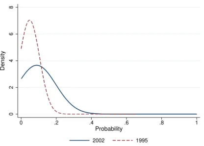
2.6shows the distribution of predicted college probabilities for the 2002 households us-ing both sets of estimated coefficients. The distribution shifts to the right when usus-ing the
2002 coefficients. After the 1999 college expansion, the predicted probability of attending
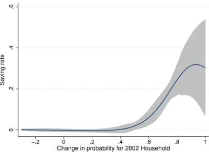
(Fan and Gijbels, 1996) of the residuals against the change in college probability. The curve lines up closely with the predictions of my theoretical model. Small increases in
college probability appear to be less correlated with saving. However, once the change
becomes large enough, saving rates are higher, too. I next estimate this relationship using
a quasi-difference-in-differences approach, in order to net out unobservable factors for
households experiencing different changes in college probability.
2.6.2 The Main Empirical Findings
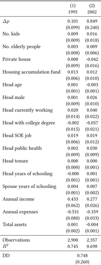
Table2.2reports the main regression results based on Equation (2.6). The estimate ofπ (the marginal effect of the change in college probability) for the 2002 sample equals 0.849.
The effect on saving is quantitatively large and statistically different from 0 at better than
the 1 percent significance level. Households for which the probability of attending
col-lege went up saved more. The estimate for the 1995 sample is much smaller (0.101)
al-though still positive. Recall, the 1995 sample was not (yet) actually subject to the college
expansion, while the 2002 sample was. Thus, I interpret the difference in the two
coef-ficient estimates as the effect due to the policy change. This ‘difference-in-differences’
(DD) estimate equals 0.748, and it is statistically different from zero. Taken literally, the
DD estimate implies that, on average, a 10 percentage point (policy driven) increase in the expected probability of college increased the typical households saving rate by about
7.5 percentage points. This effect is very large, but given the dramatic increase in saving
observed in China after 2000, it is not implausible. Also note, the impact on aggregate
saving is not straightforward to calculate because households with older children or no
children likely reacted to the policy changes, possibly through general equilibrium effects
on future employment or wages.
Table2.3reports two sets of robustness checks.12 All the regressions include the full set of controls, but I do not report the coefficient estimates to save space. In the first set
(columns 1-4), I drop households residing in Beijing (columns 1 and 2) and Beijing and Chongqing (columns 3 and 4). Dropping Beijing and Chongqing is somewhat arbitrary,
but the estimates for the changes in college probability are largest for households in these
two provinces, on average (see Figure2.5and Appendix Table C.2). The resulting DD es-timates are smaller than the main DD eses-timates; however, the estimated effect is still very
large and statistically significant. I retain the households from Beijing and Chongqing in
the remainder of my analysis.
12
As an additional robustness check, I also have conducted a standard placebo check by randomly assigning households to different provincial enrollment rates. I find no significant impact on saving, providing additional support for the main results.
The measure of the saving rate could be partially determined by transitory shocks to household income (Carroll and Samwick, 1998). Following a strand of literature, in
the second set of robustness checks (columns 5 and 6), I replace my dependent variable
in Equation (2.6) with a measure of each household’s cumulative saving rate.13 The 1995 CHIP survey asks about annual income going back to 1990 and the 2002 survey asks about
income every year starting with 1998. I aggregate each household’s previous 4 years’
in-comes to form a measure of permanent income, in order to average out transitory shocks.
Then, the cumulative saving rate is defined as Wi
Ii
, where Wi is household’s total assets reported in the survey year andIiis my measure of permanent income. With this set-up, the coefficient on∆prepresents the impact on this accumulated saving rate. Again, I find that the increase in college probability leads households to save more. Overall, the results
across the robustness checks reported in Table2.3reinforce the main results. The num-ber of observations is less than in the main regressions (note, for columns 5 and 6, I drop
households that do not report wealth), but the effects remain statistically significant and
quantitatively large.
The empirical results in Tables 2.2and 2.3are consistent with the intuition coming out of my structural model that low-saving households (S < τ) experiencing a large enough increase in the likelihood of college (p) will start to save more (i.e. Proposition 1). However, the model also implies that high-saving households could react to the college
expansion by saving less (see Appendix A). In other words, the model suggests a difference in the effect on families with ample savings versus those with little. I can use the data along
with the difference-in-differences approach to check this implication from the structural
model.
To this end, I first regress gross savings (rather than saving rates) on the full set of
observables and province fixed effects, separately for each year. i use the 1995 coefficient
estimates to predict counterfactual saving levels for households in 2002 (and vice versa).
Based on these predicted savings, I classify households into low savings (bottom quartile)
and high savings (top quartile). Then, I re-run the main regressions for each group in each
year.
tunities increase. The DD estimates further indicate that an increased college probability leads high-saving households to save less, while low-saving households save more.14
I end this section by revisiting the identification strategy. A critical assumption for
the difference-in-differences framework is that the differentially treated groups were not
trending (before the treatment) in ways correlated with the treatment.15 In my case, the
concern is that the types of households experiencing large increases in their college
prob-ability were also the types of households already increasing their savings, anyway. This
concern is valid, and I can even imagine that the policy makers might have wanted to
target the treatment towards households with increasing rates of savings because these
households would be most able to pay for college. With the cross-sectional data at hand, I cannot directly check the micro-data for pre-trends; however, I can take a more
aggre-gated look at the data. Figure 2.8 plots changes in the average household saving rate before the education expansion (from 1995 to 1998) against enrollment rates during the
enrollment increase (1998 to 2002), for each province. There exists little correlation, and
the fitted line actually reveals a slightly negative relationship. In other words, the policy
did not selectively increase enrollment rates more for the provinces in which saving rates
were already growing the most before the policy was enacted. Recall that the
household-level estimates for the change in college probability (Equation (2.7)) were a function of the provincial enrollment rates. So, from this perspective, the treatment on individual
house-holds does not seem to depend on their pre-policy saving behavior. Thus, I conclude that the analysis is not picking up pre-trends, but, instead, the saving behavior is driven by
the response to changing college opportunities.
2.7 Other Explanations for China’s High Saving Rates
This section examines the other main explanations for China’s high household saving
rates put forth in the literature (see Section3.3). First, I examine policy changes enacted around the same time. Then, I examine demographic changes. As noted above, the
regres-sions already include a number of controls aimed at accounting for these related factors.16 Moreover, I think these other factors were unlikely to be linked to the pattern of increased
college opportunities. However, since the policy reforms and demographic changes were
14
Note, these results are consistent with the main findings, Table2.4omits the middle two quartiles and focuses on gross saving rather than saving rates.
15
Another critical assumption is that households did not select into experiencing a higher increase in college probability, for example, by moving across provinces. This is unlikely to have occurred because of the speed of the policy implementation and the Hukou restrictions on migration. Just to be sure, I have checked that the results do not change when I remove the few households in the sample that changed their Hukou after the policy.
16
The main regressions also allow the coefficient estimates on these controls to change over time.
so big and also impacted household saving, I now go beyond simple control variables and allow for interactions with the variable of interest. Throughout the many specifications,
the impact of higher education expansion on saving rates remains large and statistically
significant.17
2.7.1 Other Reforms
I begin by interacting the change in college probability (allowing for heterogeneous
ef-fects) with the variables related to three other large reforms: SOE reform, housing reform, and healthcare reform. Specifically, we estimate
SRij =Wij0 δ+π·∆pij +φ·Zij +ψ·∆pij ·Zij+λj +uij, (2.9)
where Zij represents a dummy variable capturing either SOE job status, public health coverage, or private house ownership (each is considered separately). Vector W is the vector X, including all covariates except Z.18 Then, ∂SRij/∂∆p = π +ψ ·Zij is the marginal effect for each household. I report the average marginal effects, based off of the marginal effects across differentZij’s. I am interested in whether controlling for the heterogeneous impact acrossZ(i.e. the exposure to other reforms) alters the estimate (π) for the education expansion effect, and I find that it does not.
Employment at a State-Owned Enterprise (SOE)
Public sector jobs used to be part of the so-called “iron rice bowl” of social support. The
SOE reform in the 1990s, however, led to massive layoffs and made even incumbent SOE workers less secure in their employment. As discussed above, several papers have shown
that the new risk led to an increase in precautionary saving. If the households that
expe-rienced large increases in the likelihood of college were also facing greater employment
risk, then the estimates could be conflating the two channels. Columns (1) and (2) of Table
2.5provide evidence against this possibility. The coefficient estimate for∆p(0.786) in 2002 is high, even after controlling for the interaction with SOE status. Note, the interaction
Public Health Coverage
Healthcare is another motive for precautionary saving (Chamon and Prasad, 2010), as
well as life-cycle saving. Access to public health coverage has been in flux in China due
to policy changes, migration and Hukou regulations, and population aging. Columns (3)
and (4) of Table2.5report estimates controlling for heterogeneous effects based on having public health coverage. The resulting DD estimate of 0.89 is actually slightly higher than
the baseline estimate. Interestingly, the coefficient estimate for the interaction term flips signs and becomes statistically insignificant after the college expansion.
Home Ownership
China also reformed its housing market in the 1990s. By 1998, most families were allowed
to own their homes, and many households saved in the form of housing or in order to
buy housing (required down payment rates were high). Again, as with the other reforms,
I think that a connection between housing reform and exposure to the higher education
expansion is unlikely at the household level. Columns (5) and (6) in Table2.5 indicate that controlling for the interaction between the change in college probability and home
ownership has little impact on the main estimate. The DD estimate (0.80) remains very
large.
2.7.2 Household Demographics
I next consider regressions that control for interactions with variables capturing
house-hold demographic characteristics. I still apply the approach embodied in Equation (2.9), lettingZ represent the various demographic factors of interest.
Number of Children
China enacted the One Child Policy in 1978, although enforcement of the policy varied
over time and by location. Several papers have shown that Chinese households with fewer children (i.e. one) tend to save more and have drawn a connection between China’s
fertility policies and high saving rates. One reason why single child households might save
more is to invest in their child’s college education (a quantity/quality tradeoff similar to
Becker and Lewis(1973a)). In order to examine the potential heterogeneous effect across
households with different numbers of children, I define a new variableSinglethat is equal to one if there is only one dependent child and zero if there are two or more children. We
re-estimate Equation (2.9), interacting the new variable (Z = Single) with the change in the probability of college.
Table 2.6columns (1) and (2) present the results. The resulting DD estimate for the average marginal effect equals 0.77, close to my baseline result. Note, the coefficient
es-timate onSingle, while not statistically significant, is close to 0.024 both before and after the education expansion. This estimate is similar to that inLugauer, Ni, and Yin(2017);
they estimate a 2.4 percentage point decrease in saving rates due to each additional child
using a different data set and different estimation methodology.
Sex Composition
Some Chinese households may prefer having a son over a daughter because sons
tradi-tionally support their parents in old age. Relatedly, the One Child Policy may have led
to the gender imbalance now prevelant in China. Households with sons invest
differ-ently for their child’s education and also for marriage and housing purposes. Wei and
Zhang(2011) show that these factors have had a large impact on household saving rates
in China.19 Therefore, I next interact college probability with a variable (Z =Male) that equals one if a household has only male children and is zero otherwise. I count mixed
gender households (of which there are few) as non-male households. Columns (3) and (4)
of Table2.6suggest that the male child affect is quite small. Moreover, the estimate of the college expansion effect (DD=0.76) remains large.
Life-Cycle Saving and Age Effects
Simple life-cycle theory predicts that households of different ages can have different
sav-ing patterns. The younger households in my sample (household head with an age closer
to 25) might be net borrowers, while older households (age close to 60) rapidly
accumu-late assets in anticipation of retirement. The older the household head, the closer the
child is to college age, on average. To address this, I next interact the household head’s age (Z = Age) with the change in college probability. Columns (5) and (6) of Table2.6
present the results. Once again, the DD estimate (0.88) remains similar to the baseline
result.
In summary, the 1999 higher education expansion had a large effect on household
2.8 Conclusion
In this paper, I exploit the policy-induced increase in college enrollment to estimate the
impact on household saving rates in China. I find that the expansion in higher education
resulted in higher household saving rates, especially for previously low-saving
house-holds experiencing a large increase in the probability of sending their children to
col-lege. Through this saving channel, the college expansion likely affected China’s economic
growth rate and international capital flows. The findings are robust to a host of
specifi-cation modifispecifi-cations, as well as to controlling for other concurrent policy changes and on-going demographic changes.
China’s education expansion was unique in several ways. The policy change was large
and swiftly implemented, and college enrollment levels were relatively low before the
re-forms. Also, China had strict fertility controls at the time, effectively shutting down the
quantity channel in the classic fertility theory of a quantity/quality trade-off. These
char-acteristics helped inform my estimation strategy, but it remains a question as to whether
the findings are applicable to other countries and situations. Similarly, my regressions
necessarily capture the short run responses, from when the policy was new and
unex-pected, rather than the long-run response. I leave an exploration of these important is-sues to future research. However, the story is straightforward. Households save to pay
for college. The cost of higher education went up significantly despite the rapid growth of
household income. Student loans were not readily available in the early stage of the
ex-pansion and Chinese households must finance their child’s education out of their
accumu-lated savings. I believe this example may also shed lights on how education opportunities
shape household saving behaviors in other countries where households are credit
con-strained. Many countries are debating whether to increase higher education enrollment
while questioning where the funding will be. Since the return of college education exceeds
the cost according to many studies (Li,2004;Li and Xing,2010), households save more to support child’s college education. Expanding higher education means that more families
will expect their children to attend university; hence, these households save more.