On the Stablity of the Wealth Effect

Full text

(1)“On the Stability of The Wealth Effect” Fernando Alexandre Pedro Bação Vasco J. Gabriel NIPE WP 14 / 2005.

(2) “On The Stability of the Wealth Effect”. Fernando Alexandre Pedro Bação Vasco J. Gabriel NIPE* WP 14 / 2005. URL: http://www.eeg.uminho.pt/economia/nipe/documentostrabalho.php. *. NIPE – Núcleo de Investigação em Políticas Económicas – is supported by the Portuguese Foundation for Science and Technology through the Programa Operacional Ciência, Teconologia e Inovação (POCTI) of the Quadro Comunitário de Apoio III, which is financed by FEDER and Portuguese funds..

(3) On the Stability of the Wealth Effect∗ Fernando Alexandre† Department of Economics and NIPE, University of Minho, Portugal. Pedro Bação Faculty of Economics and GEMF, University of Coimbra, Portugal. Vasco J. Gabriel Department of Economics, University of Surrey, UK and NIPE 8th September 2005. Abstract Evidence of instability of the wealth effect in the USA is presented through the estimation of a Markov switching model of the long-run aggregate consumption function. The dating of the regimes appears to bear relation to movements in asset prices. A model-based explanation of the findings is suggested, highlighting the importance of the short-run relation between consumption, income and wealth in explaining the estimated long-run coefficients.. Key Words: Parameter instability; Markov switching; Consumption; Wealth effect JEL Classification: E21; E44; G10 ∗. The authors are grateful to Piergiorgio Alessandri, John Driffill, Zacharias Psaradakis, Ron Smith, Martin. Sola and other participants in the workshop “Monetary Policy and Asset Prices”, held at the University of Minho, for helpful comments. The usual disclaimer applies. The authors also acknowledge financial support from Fundação para a Ciência e a Tecnologia, research grant POCTI/EGE/56054/2004, POCTI. † Corresponding author. Address: Department of Economics, University of Minho, 4710-057 Braga, Portugal. Email: [email protected]. Tel: + 351 253 604546. Fax: + 351 253 607635.. 1.

(4) 1. Introduction. The 1990s witnessed a remarkable increase in stock prices in the USA. Between January 1995 and September 2000, the S&P 500 stock price index rose approximately by 230 percent. According to Poterba (2000), this increase accounted for more than 60 percent of the wealth creation in the USA during that period. Boom/bust periods in stock markets, and their effects on total wealth and consumption, have raised several questions for economic analysis. In particular, there is an ongoing debate on the appropriate Federal Reserve response to movements in stock prices. Several authors have questioned the stability of the wealth effect estimates. For example, Ludvigson and Steindel (1999) estimate the wealth effect to be the usual 0.04 for their full sample, 1953-1997. However, their estimate reaches 0.1 in the 1976-1985 sub-sample, and is only 0.02 after 1986. Furthermore, Mehra (2001) corroborates the view that the estimate seems to depend on the econometric model, the measures of wealth and consumption, and on the sample. Poterba (2000) puts forward three reasons that might explain the observed signs of instability. First, the fact that only a subset of households own equity, which was the main source of shocks to aggregate wealth in that period. Second, the growing importance of equity investments that are held in tax-favored retirement accounts. Third, the falling cost of leaving bequests. In this paper we report additional empirical evidence on, and provide an explanation of, the instability of the wealth effect. The paper is structured as follows. In the next section we use a simple cointegrated Markov switching model, which allows us to distinguish endogenously between periods with different values for the wealth effect estimate. We relate these sub-samples to periods with different levels of volatility in asset prices. We then present in section 3 a model-based explanation of the econometric results. Section 4 concludes.. 2. Empirical Analysis. The standard derivation of the “consumption function” (see, e.g., Lettau and Ludvigson, 2001, LL henceforth) begins by assuming that consumption tends to a stationary fraction of total wealth, which allows us to write a cointegrating relation between (the logs of) consumption (ct ) and total wealth (wt ): ct − wt = ut , 2. (1).

(5) where ut is a stationary process. Such a result may be obtained from the usual micro-founded model of consumption (e.g., Campbell and Mankiw, 1989) if one assumes that the period utility is well approximated by a log function of consumption. The derivation then proceeds to separate total wealth into human and non-human wealth wt ≈ ωat + (1 − ω) ht ,. (2). where at is log non-human wealth, ht is log human wealth and ω is the average weight of nonhuman wealth in total wealth. Since human wealth is not observable, LL (2004) show that an approximation1 may be obtained by using labor income, yt , as a proxy for ht , resulting in the following log consumption-wealth ratio ct − ωat − (1 − ω) yt = u∗t .. (3). These authors show that ct , at and yt share a common trend, with normalized cointegration vector (1, −β, −δ) and cointegration residual ct − βat − δyt (cayt in brief)2 . The coefficient β is interpreted as the “wealth effect”, their estimation yielding β̂ = 0.3 and δ̂ = 0.6. LL (2004, section 4) discuss the stability of the long run relationship, resorting to the sup, mean and Lc tests of Hansen (1992), which produced ambiguous results. Indeed, sequential tests of this family may not be able to detect certain types of structural change, such as Markov regime shifts or threshold effects, as shown by Carrasco (2002). Therefore, a simple way of assessing instabilities in the consumption-wealth ratio is to allow the relationship to undergo occasional discrete shifts of the Markov switching type, as suggested by Hall, Psaradakis and Sola (1997). Thus, we specify the cointegration equation as ct = µst + βst at + δst yt + ηst εt ,. (4). where {εt } is a stationary random sequence with mean zero and unit variance, while st is a discrete-valued random variable, independent of εt−i for all i. This variable indicates the unobserved regime operative at time t, forming a homogeneous first-order Markov chain with state space {0, 1} and transition probabilities p = Pr(st = 1|st−1 = 1) and q = Pr(st = 0|st−1 = 0). 1 2. See LL (2001 and 2004) for a more detailed discussion of the assumptions employed in the approximation. Note that the coefficients β and δ need not sum to 1, since non-durable consumption and services are used. as a measure of total consumption.. 3.

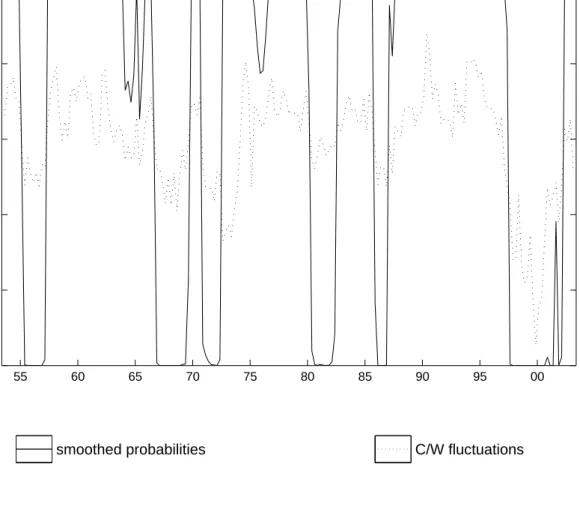
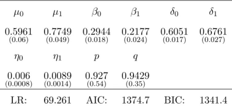
(6) Notice that the formulation in (4) is very flexible, in that it allows the data to determine when and which parameters have shifted, be it the long run coefficients or the variance (see Hall et al., 1997, for more details on the use of MS models in a cointegration setting). Other papers (Ludvigson and Steindel, 1999 and Mehra, 2001, for example) have relied on an ad-hoc choice of break points. This model, however, will be able to distinguish endogenously periods where, for instance, asset markets and returns may be behaving differently. This is particularly convenient to study the implications of the theoretical model developed in the next section. Table 1 records the results of maximum likelihood estimation of the parameters of model (4) and respective asymptotic standard errors3 . Both the LR test and the model selection criteria favour the MS model over the linear cointegration specification4 . The MS model identifies two distinct regimes: regime 1 is associated with more volatile periods, which roughly coincide with historical ”bull” markets, such as those of the late 1960s and 1990s, while regime 0 is associated with ”calmer” periods. Figure 1 shows the smoothed probabilities produced by the MS model, plotted against fluctuations in the consumption-wealth ratio as estimated by LL (2004), confirming the view that the identified regimes seem to capture the state of asset markets and of the economy. In state 1, the coefficient associated with asset wealth is smaller (0.22) than in state 0 (0.29), which is consistent with the empirical evidence surveyed in Poterba (2000) and Mehra (2001). It is interesting to notice that the difference between the β’s and the δ’s across regimes is approximately the same (0.07). Although these fluctuations do not appear to be sizeable, the cointegration vector estimated by LL (2004) seems to be a “composite” estimate of the different regimes. The next section presents additional possible explanations for the documented instability.. 3. Model-Based Explanation. LL (2001) note that the estimated coefficients (0.3 and 0.6) are what one would expect if the aggregate production was well represented by a Cobb-Douglas, since they are very close to the 3. We resort to the same dataset used in LL (2004), comprising quarterly data on aggregate consumption, asset. wealth and labor income, spanning from 1951:4 to 2003:3. 4 AIC and BIC values for the linear model are −1248.2 and −1234.8, respectively.. 4.

(7) usual income shares of capital and labor. In fact, if aggregate output is Ot = Ktα L1−α , t. (5). then labor income is Yt = (1 − α) Ot and the return to capital is Rt = αOt . Now note that a standard macroeconomic asset-pricing model would imply ¶ µ Qt+1 + Dt+1 , Qt = Et 1 + rt. (6). where Qt is the asset price, Dt are “dividends” and rt is the discount rate. In steady state, one obtains Q=. ξ D, 1−ξ. (7). where ξ is a risk-adjusted discount factor. Noting that non-human wealth is A = (Q + D) K (cum-dividend price times asset volume) and that the product D × K is just the steady-state return to capital, then A = (Q + D) K =. α D K= O. 1−ξ 1−ξ. (8). If we write consumption as C = O − X, where X stands for other uses of aggregate output, then for an arbitrary θ C =O−X =θ. 1 1−ξ A + (1 − θ) Y − X. α 1−α. (9). This seems to suggest that, in the long run, consumption is not related to labor income and non-human wealth alone, but also to other components of aggregate output. One implication of this is that, to be able to restore the original result, one must expect X to be somehow related to A and Y , so that it may be substituted out. One way to proceed would be to assume that A and Y capture the nonstationarity in X. Stability of the wealth effect would then have to rely on the stability of the relation of the components of X, for instance, government spending, to A and Y — given the time span covered by the data, this would appear dubious. But assume that this problem can be solved in the most simple way: set X = 0, which leads to the same conclusions as assuming that consumption is a constant fraction of output. In this case C=θ. 1−ξ 1 A + (1 − θ) Y, α 1−α. (10). i.e., if we run the usual regression in levels, the “wealth effect” is indeterminate, since θ is arbitrary. Nevertheless, it is common to run the regression in logs. In this case the usual first 5.

(8) order Taylor approximation gives (ignoring a “constant”) c = ρa a + ρy y,. (11). where the coefficients are ρa = ρy =. θ 1−ξ O α A = θ = θ, C C 1 (1 − θ) 1−α Y O = (1 − θ) = 1 − θ. C C. (12) (13). Taken literally, the Taylor approximation would imply the sum of the coefficients to equal unity. The fact that it is just an approximation may explain why this is not the case in the data — Jensen’s inequality could be the reason for this. Nevertheless, our results in section 2 are consistent with matching symmetric variations in the coefficients, corresponding to changes in θ. What matters to us here is that again the aggregate long-run wealth effect is indeterminate. If this was really the case, one would expect the estimated coefficients to depend on short-run correlations between the variables. This would result in instability of the coefficients as one varied the sample. To see this, note that the previous equations relate steady state values. Let the actual values be c̃t = c + εct ,. (14). ãt = a − εat ,. (15). ỹt = y − εyt ,. (16). where the added disturbances reflect short-run deviations from the steady state. Then c̃t = ρa ãt + ρy ỹt + ρa εat + ρy εyt + εct .. (17). Minimisation of the variance of the residual, V [ρa εat + ρy εyt + εct ] with respect to θ leads to the following estimate of the wealth effect ρa = θ =. σyy − σya + σyc − σac , σyy + σaa − 2σya. (18). ³ ´ where σij = E εit εjt , with i, j = c, a, y, represent variances and covariances in the short run. This result and the reasoning leading to it suggest there may be reasons for concern regarding the relevance of empirical estimates of the wealth effect in the context of this model. The estimates may reflect short-term correlations, possibly mixed with long-run parameters, as in 6.

(9) the regression in levels. In particular, notice that, ceteris paribus, an increase in the variance of asset wealth reduces the size of the estimated wealth effect — this is exactly what the data, as reported in section 2, shows. We developed our model from the point where LL (2001) stopped. These authors estimated the consumption equation and concluded it was consistent with the usual estimates of labor and capital income shares. We have shown that if we accept this conclusion, then the consumption function is likely to show signs of instability, and in the simple case studied here it would even lead to indeterminacy. The reader may ask whether the issue is only about relating the estimates of the consumption-function coefficients to labor and income shares. It is not. If we accept the assumptions of the standard derivation of the wealth effect — that consumption tends to a stationary fraction of wealth, that the average weight of human wealth on total wealth is stationary and that labor income captures the non-stationarity in human wealth — then the algebra of I(1) variables says we should also conclude that there is cointegration between any two-element combination of consumption, wealth and labor income. This is in fact another instance of indeterminacy, but one that apparently is not upheld by the data. On the other hand, the implications from the model we have just presented, in particular that the wealth effect should be unstable, do in fact appear to be matched by the data, as reported in section 2. In view of the indeterminacy/instability result, what is surprising is actually the relatively small variation across regimes of the estimates reported in section 2. The empirical results and the theoretical model taken together suggest that there may be some structure in the short-run correlations between consumption, income and asset wealth — i.e., consumption, income and asset prices, which drive asset wealth in the short-run. This short-run structure reduces the magnitude of oscillation in the estimated coefficients (possibly making the traditional cointegrating relation a useful reference point), but also makes them react in a particular way to movements in asset prices. To sum up, the usual derivation of the consumption cointegrating relation itself suggests that the estimated coefficients may be changing over time. The simple model investigated here adds to this a possible connection, through short-run correlations, between asset wealth (i.e., asset prices) and these coefficients. This warrants a more detailed study of the short-run relation between these variables, which is the subject of Gabriel, Alexandre and Bação (2005).. 7.

(10) 4. Conclusion. This paper documents patterns and sources of instability in the consumption-wealth ratio. We estimated a simple Markov switching model and found different estimates of the wealth effect associated with two regimes. These regimes seem to correspond to periods of high/low volatility in asset prices. This suggests that consumption reacts differently to asset prices depending on whether these changes are perceived to be permanent or transitory. We then show that the instability is not surprising given the way the consumption equation is derived. In this way, we add to the explanations given in Poterba (2000) a model-based reason for instability in the wealth effect. The magnitude of parameter instability is relatively small, and linear cointegration may perhaps be capturing the fundamental path of the relationship. Indeed, in a related paper (Gabriel et al., 2005), we suggest that short term asymmetries, not long run instability, may be more important in describing the dynamics in this trivariate system.. References [1] Campbell, J. Y. and Mankiw, N. G. (1989), Consumption, Income and Interest Rates: Reinterpreting the Time Series Evidence, in Olivier J. Blanchard and Stanley Fischer, eds., NBER Macroeconomics Annual: 1989, Cambridge, MA, MIT Press, 185-216. [2] Carrasco, M. (2002), Misspecified Structural Change, Threshold and Markov Switching Models, Journal of Econometrics, 109, 239-273. [3] Hall, S. G., Psaradakis, Z., Sola, M. (1997), Cointegration and Changes in Regime: the Japanese Consumption Function., Journal of Applied Econometrics, 12, 151-168. [4] Hansen, B. E. (1992), Tests for Parameter Instability in Regressions with I(1) Processes, Journal of Business and Economic Statistics, 10, 321-335. [5] Gabriel, V. J., Alexandre, F. and Bação, P. (2005), The Consumption-Wealth Ratio under Asymmetric Adjustment, unpublished manuscript. [6] Lettau, M. and Ludvigson, S. (2001), Consumption, Aggregate Wealth and Expected Stock Returns, Journal of Finance, 56, 815-849. 8.

(11) [7] Lettau, M. and Ludvigson, S. (2004), Understanding Trend and Cycle in Asset Values, American Economic Review, 94, 276-299. [8] Ludvigson, S. and Steindel, C. (1999), How important is the stock market effect on consumption?, Economic Policy Review, Federal Reserve Bank of New York, 5, 29-51. [9] Mehra, Y. P. (2001), The Wealth Effect in Empirical Life-Cycle Aggregate Consumption Equations, Economic Quarterly, Federal Reserve Bank of Richmond, 87, 45-68. [10] Poterba, J. M. (2000), Stock Market Wealth and Consumption, Journal of Economic Perspectives, 14, 99-118.. 9.

(12) 5. Appendix Figure 1: Regime 0 probabilities and C/W fluctuations 1. 0.04. 0.8. 0.02. 0.6. 0. 0.4. −0.02. 0.2. −0.04. 0. 55. 60. 65. 70. 75. 80. smoothed probabilities. 85. 90. 95. C/W fluctuations. 10. 00. −0.06.

(13) Table 1: Markov switching cointegration estimates µ0. µ1. β0. β1. δ0. δ1. 0.5961. 0.7749. 0.2944. 0.2177. 0.6051. 0.6761. η0. η1. p. q. 0.006. 0.0089. 0.927. 0.9429. LR:. 69.261. AIC:. 1374.7. BIC:. 1341.4. (0.06). (0.0008). (0.049). (0.0014). (0.018). (0.024). (0.54). (0.017). (0.027). (0.35). 11.

(14) Most Recent Working Papers NIPE WP 14/2005. Alexandre, Fernando, Pedro Bação and Vasco J. Gabriel, On the Stability of the Wealth Effect, 2005.. NIPE WP 13/2005. Coelho, César, Francisco José Veiga and Linda G. Veiga, Political Business Cycles in Local Employment, 2005.. NIPE WP 12/2005. Veiga, Francisco José and Ari Aisen, The Political Economy of Seigniorage, 2005.. NIPE WP 11/2005. Silva, João Cerejeira, Searching, Matching and Education: a Note, 2005.. NIPE WP 10/2005. de Freitas, Miguel Lebre, Portugal-EU Convergence Revisited: Evidence for the Period 1960-2003, 2005.. NIPE WP 9/2005. Sousa, Ricardo M., Consumption, (Dis) Aggregate Wealth and Asset Returns, 2005.. NIPE WP 8/2005. Veiga, Linda Gonçalves and Maria Manuel Pinho, The Political Economy of Portuguese Intergovernmental Grants, 2005.. NIPE WP 7/2005. Cortinhas, Carlos, Intra-Industry Trade and Business Cycles in ASEAN, 2005.. NIPE WP 6/2005. Mourão, Paulo Reis, Que Critérios Redistributivos na Lei das Finanças Locais?, 2005.. NIPE WP 5/2005. Mourão, Paulo Reis, Elasticities of Regional and Administrations Expenditures – the Portuguese case, 2005.. NIPE WP 4/2005. Mourão, Paulo Reis, Incentivos à Localização em Trás-os-Montes e Alto Douro (os séculos XII – XVI), 2005.. NIPE WP 3/2005. Alexandre, Fernando and Pedro Bação, Monetary Policy and Asset Prices: the investment channel, 2005.. NIPE WP 2/2005. Conraria, Luís Aguiar and Yi Wen, Understandig the Impact of Oil Shocks, 2005.. NIPE WP 1/2005. Bleaney, Michael and Manuela Francisco, Inflation Persistence and Exchange Rate Regimes: Evidence from Developing Countries, 2005.. NIPE WP 15/2004. Ribeiro, José Cadima, José Viseu, Tânia Delalande and Cristina Rodrigues, UEFA Euro 2004 Visitor Analysis, 2004.. NIPE WP 14/2004. Ribeiro, José Cadima, José Viseu, Tânia Delalande and Cristina Rodrigues, UEFA Euro 2004 Tourism Impact Analysis, 2004.. Local.

(15)

No results found