Wellesley College
Wellesley College Digital Scholarship and Archive
Honors Thesis Collection
2016
A Computational Approach to Foreign Accent
Classification
Emily Ahn [email protected]
Follow this and additional works at:https://repository.wellesley.edu/thesiscollection
This Dissertation/Thesis is brought to you for free and open access by Wellesley College Digital Scholarship and Archive. It has been accepted for inclusion in Honors Thesis Collection by an authorized administrator of Wellesley College Digital Scholarship and Archive. For more information, please [email protected].
Recommended Citation
Ahn, Emily, "A Computational Approach to Foreign Accent Classification" (2016).Honors Thesis Collection. 323.
1
A Computational Approach to Foreign Accent Classification
Emily Ahn
Submitted in Partial Fulfillment of the
Prerequisite for Honors in Cognitive and Linguistic Sciences
May 2016
2
Acknowledgments
In the first week of classes last fall, I walked into Sravana Reddy’s office and met her for the first time. From that spontaneous moment when I had asked her, “Can I thesis with you?” till now, she has inspired me and brought me full-force into the realm of natural language and speech processing, all with incredible patience and grace. I thank her for her persistence in constantly trying new ideas, and for showing me the intersection of my favorite interests: Computer Science and Linguistics.
I also thank my professors for their trust and encouragement. To Sohie Lee, my dearest major advisor who responds to emails at the speed of lightning and provides Haribo gummy bears during office hours. To Angela Carpenter, who taught my favorite classes at Wellesley (Phonetics/Phonology, and Invented Languages) and whom I admire for her strength and elegance. And to the rest of my thesis committee, Margery Lucas and Eni Mustafaraj, who have taken a genuine interest in this thesis and have offered their guidance and advice.
I want to thank my crew team—you all have taught me the definition of resilience and what it means to push your limits and surprise yourself. And to my ICF community—you have been a source of stability and encouragement to
challenge me in my faith. To my dearest friends—I know that the relationships that I’ve made here at Wellesley will be a foundation for the rest of my life.
To my family—how can I even describe how much your love and support mean to me? Thank you for showing me how to live a balanced lifestyle and how to appreciate every moment. Thank you for believing in me and reminding me that rest is important, and that everything will work out in the end.
Lastly, I couldn’t do anything without the grace of God. Thank You for giving me life and giving me peace.
3
Abstract
As speech recognition and intelligent systems are more prevalent in society today, we need to account for the variety of accents in spoken language. An
important step involves identifying the type of accent given a sample of speech. For this thesis, we have coded1 machine learning algorithms to classify accents from
foreign-accented English. Given a data set of 4925 phone calls that span 23 different accents, we have trained Gaussian Mixture Models for each accent with two main methods. The text-independent classifier assumes that we took sound features without knowing the transcriptions of the speech, while the text-dependent
classifier relies on transcriptions in order to align each phoneme (or sound unit, e.g. /AH/ and /K/) to its utterance in the data. We acquired these transcriptions by releasing tasks via Amazon Mechanical Turk for the following 7 accents: Arabic, Czech, French, Hindi, Indonesian, Korean, and Mandarin. Upon evaluation, we found that a 7-way accent identification task achieved an accuracy rate of 41.38% for the text-independent classifier and 45.12% for the text-dependent classifier.
4
Table of Contents
1 – Introduction ... 5
2 – Prior Work ... 7
3 – Data ... 10
4 – Methodology and Results ... 13
4.1 – Feature Extraction ... 13
4.2 – Text-Independent Classifier ... 13
4.2.1 – Averaging across all time frames ... 14
4.2.2 – Testing with subsets ... 14
4.2.3 – Testing with all 23 accents ... 15
4.3 – Text-Dependent Classifier ... 17 4.3.1 – Acquiring Transcriptions ... 18 4.3.2 – Formant Classifier ... 20 4.3.3 – Forced Alignment ... 20 4.3.4 – Phoneme Classifier ... 20 4.4 – Confusion Matrices ... 27 4.5 – Phoneme Analysis ... 28 5 – Conclusion ... 30 5.1 – Summary ... 30 5.2 – Further Discussion ... 30 5.3 – Future Work ... 31 References ... 34
5
1. Introduction
We see a publicly available Foreign Accent Classification system as an increasingly important feature for current speech technologies. Given that we live in a country that is so international with about 13% of the U.S. population being foreign-born2, we must provide services to people who speak with different accents.
Disability services, like offering automatic subtitles for conferences, would be aided by a system that accounts for varying accents. Areas such as immigration and national security would also benefit from automated systems that could detect English speakers of Mandarin Chinese, Arabic, and many other linguistic backgrounds. Furthermore, a refined accent classifier could eventually have features that help English-learners recognize aspects of their own foreign accents.
Existing automatic speech recognition (ASR) systems for English have been trained on a wide array of American-accented speech, so we see technology like Apple’s Siri and Google Now perform quite well on understanding native American English speakers. Yet there is much less training data for ASR systems to learn from foreign-accented speakers. With the goal of making these systems more robust, one way to recognize speech (i.e. convert speech to text) that is from a non-standard accent of English is to first classify which accent it is. This task is similar to
Language Identification (LID) but in other ways more challenging (Chen et al., 2010). In LID tasks, the phonetics are more distinct across speech from different languages, but when these non-native English speakers speak English, their first language and the English come in phonetic contact and can blend together.
This thesis aims to combine existing machine learning techniques to classify foreign-accented English speech. While research has been done on accented speech that is text-independent, nothing has been done to directly compare a classifier using untranscribed speech with another classifier that takes all phonemes
(individual sound units in language) of known transcribed speech. In order to help
6
the process of quickly obtaining these transcriptions, we use Amazon Mechanical Turk (AMT), which is a crowdsourcing web platform where individuals or
companies can pay AMT workers to complete tasks. With the transcriptions provided by these workers, we are able to train phoneme-specific models that out-perform the text-independent models.
7
2. Prior Work
The biggest inspiration for the starting methodology of this thesis was the classifier built in Choueiter et al. (2008). They used the Foreign Accented English dataset from the Center for Spoken Language Understanding in order to train Gaussian Mixture Models (GMMs) on the 23 different accents (see section 3 for information about the corpus). As a baseline, their models provided their best performance of 22% correct in a 23-way classification task. They then improved these models by implementing additional dimensionality reduction techniques such as PCA3 and HLDA4 to achieve an accuracy of 32%. For our classifier, we will first
be attempting to replicate the baseline system of a 22% accuracy using similar techniques but without PCA and HLDA for the sake of simplicity. To motivate the method in building Gaussian Mixture Models, we also use techniques from
Reynolds and Rose (1995), who trained robust GMMs for speaker identification tasks.
Gaussian Mixture Models (GMMs) are probability density functions that are popular in modeling data for both unsupervised and supervised learning. A GMM superpositions multiple distributions to model the likelihood of a point in
multidimensional space. Classification of a new test point point would go to the GMM that returns the highest probability of generating that point. We can
manipulate parameters of GMMs such as the type of covariance and the number of distributions. The covariance type (i.e. Full, Tied, Spherical, and Diagonal) will dictate the overall shape of the GMM, while the number of n distributions, or components, will determine how the model will learn and categorize similar features into n groups together. This whole process is initiated with the EM (expectation maximization) algorithm.
3 Principal Component Analysis
8
The classifier from Choueiter et al. (2008) is wide and comprehensive, but it assumes that the speech is untranscribed. While this method is useful since most speech data in the world is not transcribed, I turned to literature pertaining to transcribed speech. Angkititrakul and Hansen (2006) researched phone-based modeling for accent classification using a smaller dataset of Thai, Mandarin,
Turkish, French, and American English. They controlled the speaker variability by recording a limited set of native speakers saying the same set of utterances, and then they experimented on subsets of accents while controlling for gender. They used techniques such as Hidden Markov Models and speech trajectory models that follow articulatory space, and their overall 5-way accent classification achieved a 40.64% accuracy at best. Notably their results suggested that accents whose languages are closer in the world language tree might be similarly classified. The styles of experimentation and comparison, as well as use of transcribed phonemes, will provide inspiration for this thesis.
With an even smaller dataset from native speakers of Mandarin and native speakers of American English, Sangwan and Hansen (2012) were able to use phoneme-based models and an implementation of phonological rules in order to classify between the two accents. Using precise phonological features allowed them to identify the direct sounds that native Mandarin speakers have trouble with when speaking English. This study offers insight into how we could use a priori
phonological rules to better identify and expect sound changes that carry over from a native language into a second language.
Much after we compiled literature from which to base our own research, we discovered a paper released in early 2016 that closely mirrored our process. Ge (2016) chose 7 accents from the CSLU FAE corpus (albeit a different subset than our 7 accents), and first replicated Choueiter et al.’s (2008) text-independent GMM system. He then acquired transcriptions and used phoneme alignment to build a Transcribed model based on vowel phonemes and their feature space. Where we deviate from this system is in the approach to the transcribed version—our
9
In order to determine a process and reasonable expectation of how much to pay AMT workers to transcribe our files, we found literature on quality-controlling for transcription-based tasks. Parent and Eskenazi (2010) combined elements of an ASR system with raw transcriptions and created a two-step process for AMT
workers to first agree or disagree with the ASR-produced transcription, and then to rewrite them. While this process is not be used in this thesis, the cost estimates were quite useful. Since Parent and Eskenazi found that it was optimal to pay workers approximately $14.50 an hour for quality transcriptions, we divide that by 2-3 minutes that we expect to take to transcribe 20 seconds of speech, and pay $0.50 per task (see section 4.3.1).
10
3. Data
All speech data used for training and testing for this research was taken from the CSLU Foreign Accented English corpus. Included in this data set are a total of 4925 phone calls, each ranging from 2 to 20 seconds (but mostly at precisely 20 seconds). The general quality of each file is good, taken at a sampling rate of 8000 Hz.
These calls span 23 different accents, as seen in Table 3-1, with each accent containing a varied number of files. The text-independent classifier uses all data from the 23 accents as well as combinations of subsets of these 23. The text-dependent classifier uses at most 7 accents.
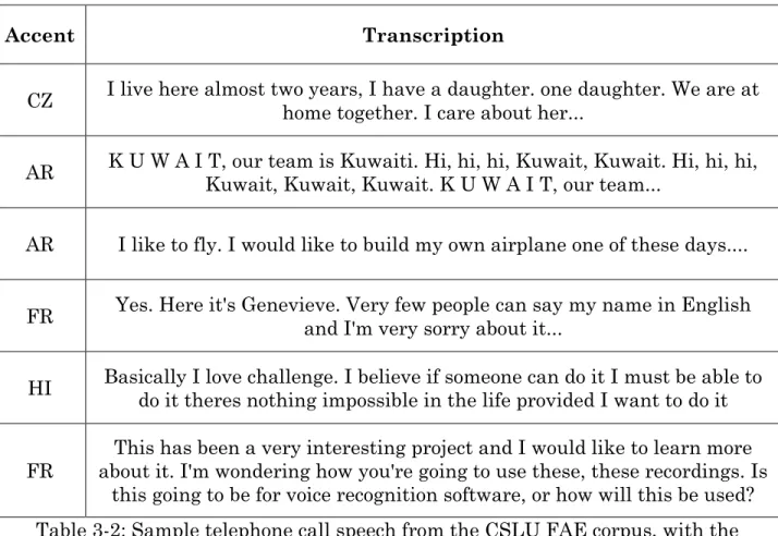
Each file consists of speech from distinct native speakers of a non-English language. They represent a wide age group and include all genders, and the spoken content is freely up to the speaker. Samples of the phone calls are transcribed in Table 3-2.
We initially assigned a random 75% of files per language to be for training and the remaining 25% to be for testing. This train-test split was kept constant across all experiments in order to evaluate the quality of different types of
classification. Although Ge (2016) used a training, development, and testing ratio of 75:15:15, we did not choose to set aside development data. This hold-out data would be useful for tuning parameters, but we believed the existing data to be too small to split into three groups.
11
Accent Abbreviation Total # Files Duration
Brazilian Portuguese BP 459 2:34:23 Hindi HI 348 1:56:09 Tamil TA 326 1:06:28 German GE 325 1:36:03 Spanish SP 308 1:05:18 French FR 284 1:31:04 Mandarin MA 282 1:30:37 Hungarian HU 276 1:27:20 Farsi FA 262 1:18:55 Cantonese CA 261 1:17:33 Russian RU 236 1:11:12 Italian IT 213 1:04:06 Swedish SD 203 1:07:37 Japanese JA 194 0:56:05 Korean KO 169 0:53:35 Polish PO 143 0:47:04 Vietnamese VI 134 0:27:11 Arabic AR 112 0:34:31 Czech CZ 102 0:33:24 Indonesian IN 96 0:31:18 Swahili SW 71 0:21:33 Iberian Portuguese PP 66 0:21:08 Malay MY 56 17:21
Table 3-1: List of 23 accents in CSLU FAE corpus, with their abbreviations and total number of files provided in order from greatest to least, and total time duration of the sound files. Rows in bold are the accents used for analysis of the
12
Accent Transcription
CZ I live here almost two years, I have a daughter. one daughter. We are at home together. I care about her...
AR K U W A I T, our team is Kuwaiti. Hi, hi, hi, Kuwait, Kuwait. Hi, hi, hi, Kuwait, Kuwait, Kuwait. K U W A I T, our team...
AR I like to fly. I would like to build my own airplane one of these days....
FR Yes. Here it's Genevieve. Very few people can say my name in English and I'm very sorry about it...
HI Basically I love challenge. I believe if someone can do it I must be able to do it theres nothing impossible in the life provided I want to do it
FR
This has been a very interesting project and I would like to learn more about it. I'm wondering how you're going to use these, these recordings. Is
this going to be for voice recognition software, or how will this be used? Table 3-2: Sample telephone call speech from the CSLU FAE corpus, with the
13
4. Methodology and Results
4.1 Feature Extraction
For the feature representation of these sound files, we extracted PLP
(Perceptual Linear Prediction) features by using the HCopy tool and running HTK (Hidden Markov Model Toolkit; Young & Young, 1993) on the wav files. This produced 52-dimensional vectors for every 25 milliseconds of speech, where the start of the speech window is shifted for every 10 milliseconds of the file. Each vector contains 13 values pertaining to 12 frequencies and 1 energy value of the acoustic sample, and 13 more features for their first derivatives, and so on up to the third derivative. This is how 1 speech window holds a total of 52 features.
We decided to keep the acoustic measurements as PLP values instead of the other common sound representations, MFCCs (Mel-Frequency Cepstral
Coefficients), because PLP features are known to be more robust when the training and testing data have different environments (Woodland et al., 1996). This should be more appropriate for the diversity within the telephone call data of the CSLU FAE corpus.
4.2 Untranscribed Classifier
In order to model the baseline in Choueiter et al. (2008), we used Numpy and Scikit-Learn5 to build a GMM that took in training files and evaluated on the
testing files.
14
4.2.1 Averaging across all time frames
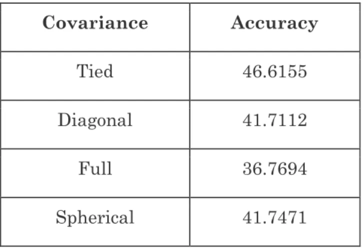
At first we took the approach of averaging PLP values over all time frames within a given file, which would collapse all vectors into a single 52-dimensional vector that would represent the features of one entire phone call, and we trained this on only 1 Gaussian mixture. However, this performed below chance, so we did not pursue this option further. Table 4.2-1 shows the results of classifying between 3 distinct accents (Arabic, Hindi, and Mandarin) by averaging over all time frames. The best classifier with Tied covariance had a 46.62% accuracy, which was lower than a chance rate of 47.03%.
Covariance Accuracy
Tied 46.6155
Diagonal 41.7112
Full 36.7694
Spherical 41.7471
Table 4.2-1: Percent accuracies of AR, HI, MA on all covariance types and by averaging PLP values over all time frames per file. Chance is 47.0270% (proportion
of HI files)
4.2.2 Testing with subsets
The better approach was to instead use each time frame of 25 milliseconds independently, where each frame (and consequently each vector) was inserted into the training model. The parameters that we manipulated when training the data on the GMMs are the number of components (i.e. mixtures) and the type of covariance.
We trained and tested on a group of 3 distinct accents (Arabic, Mandarin, and Hindi) as well as 3 similar accents (Polish, Hungarian, and Russian) in order to
15
examine what covariance types would be ideal, and we found that Full covariance always performed best, with Tied covariance as second-best.
Table 4.2-2 shows the results of classifying between Arabic, Hindi, and Mandarin, where each 25ms frame in a given sound file was treated independently and all PLP features for each frame were used. Tied and Full covariance matrices proved to be significantly better, so we stopped testing with Spherical and Diagonal covariances. This makes sense because Full covariance is the most powerful type and it captures every aspect of the data, given that there is enough data. Spherical and Diagonal types are known to be spatially more efficient but lacking in accuracy. Additionally to note from this table is that even with more components, the
performance gets better only marginally at a diminishing rate, so we did not continue to test further.
# Components Tied Diagonal Full Spherical
1 47.1779 42.4462 47.3096 42.0459
2 51.0738 45.8210 50.2746 44.2103
4 49.3236 — 51.2053 —
8 49.7261 — 51.2090 —
Table 4.2-2: Percent accuracies of Arabic, Hindi, and Mandarin, where chance is 47.0270% (proportion of HI files)
In order to test my hypothesis that the GMM classifier performs better on distinct accents than similar accents, we tested on Hungarian, Polish, and Russian. Table 4.2-3 shows that at least for 1 and 2 components, the Full covariance
accuracies are below chance, which is the proportion of Hungarian files to all 3 sets of files. This proved to be worse than the distinction between Arabic, Hindi, and Mandarin, which held an accuracy of at least 4% better than chance.
16
# Components Tied Diagonal Full Spherical
1 37.5627 31.9075 36.7930 36.9445 2 40.1607 30.8366 40.6198 40.2981
Table 4.2-3: Percent accuracies of Hungarian, Polish, and Russian, where chance is 42.0732% (proportion of HU files)
4.2.3 Testing with all 23 accents
We then trained this classifier and evaluated all 23 accents across Tied and Full covariances while incrementing the number of components by powers of 2 all the way up to 1024. This was similarly done in Choueiter et al. (2008) in order to quickly scale up the distribution space. Results in Table 4.2-4 show that after 2 components, the Full covariance always performed better than the Tied covariance. And within the Full column, there is a relative peak performance of 17.5467% (compared to a chance rate of 9.2608%) at 128 components, although 512 does marginally better.
# Components Tied Full
1 6.8237 6.6613 2 7.3111 7.2298 4 7.5548 8.2859 8 7.1487 9.2608 16 7.8798 11.4541 32 7.9610 11.7790
17 64 8.3672 15.5158 128 8.6109 17.5467 256 8.8546 16.5719 512 9.9650 17.8716 1024 10.8042 12.9163
Table 4.2-4: Percent accuracies of a 23-way classification for all accents, where chance is 9.2608% (proportion of BP in test files)
At our best, this text-independent classifier achieved a 17.8716% accuracy while the baseline in Choueiter et al. (2008) was at 22%. Because they were not explicit about the details to the feature extraction process in their paper, we believe that our system and theirs could have had discrepancies related to the train-test data split or the windowing size.
After computing these results, we have chosen 128 components and the Full covariance type to be optimal. It makes sense to approximate 3 components for about 40 total possible English phonemes to get 128 components. Even though the overall accuracy for 512 components was higher, it is likely to have overfitted the data if there was already a peak at 128. I test with both 256 and 512 components on the subsets of accents used in the text-dependent classifier to confirm this.
4.3 Text-Dependent Classifier
Our next approach was to build a classifier that would explicitly know what sounds, or phonemes, that each speaker was saying, and then use those phonemes to train and classify each accent. In order to do this, we needed transcriptions.
18
4.3.1 Acquiring Transcriptions
At first, we wanted to see if the quality of Google's ASR could accurately transcribe our sound files. Since YouTube provides automatic captions for uploaded videos, we took advantage of this service. We ran Arabic, Czech, and Indonesian through YouTube and evaluated the results. These three languages had a similar quantity of data, which were all relatively short enough to test.
However, seeing as the Google ASR results were unsatisfactory (see Table 4.3-1), we decided to obtain manual transcriptions. Because each 20 second sound file would take approximately 2-3 minutes to transcribe, we knew that scaling this work to transcribing 4925 phone calls would be a tremendous effort for one person to do. Therefore we turned to Amazon Mechanical Turk (AMT).
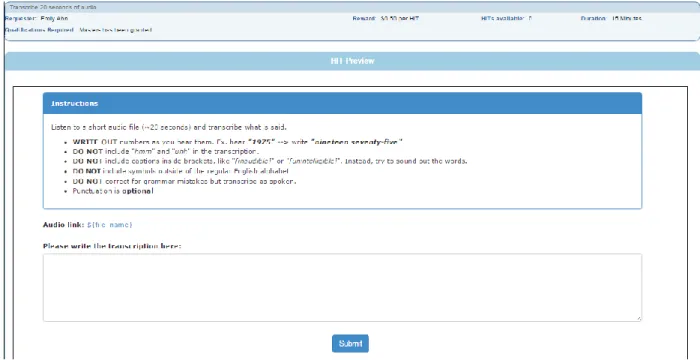
The process of releasing work on AMT included uploading all sound files to Google Drive, writing a script to store the file links in a csv file, and creating a "batch project" on our AMT account. We released a batch at a time, and paid
workers $0.50 to transcribe a 20 second file, or $0.25 to transcribe a 4-10 second file (see the screenshot image of a sample task in Figure 4-1). Due to time and budget constraints, we could only release 7 batches of accents (Arabic, Czech, French, Hindi, Indonesian, Korean, and Mandarin), which we chose from a variety of language families.
19
File Name YouTube Transcription Actual Transcription
FAR00258.wav
my parents moved to a
tournament what i said there for about sixteen years of high school after i graduated my house korea representative to the united states of america like a freshman idk
my parents moved to UAE so I went with them. I stayed there for about sixteen years. I was studying in high school. After I graduated my high school here, my parents sent me to the United States of America so I can finish my degree.
FCZ00027.wav
i come from six secrets public studied electrical engineering and computer science and artificial intelligence
I come from Czech republic which was Czechoslovakia I studied electrical engineering and
computer science over there it here I'm continuing in that in time and artificial intelligence
FIN00042.wav
like to play basketball for
jobless claims we compared to a medicolegal something but check around a computer on the internet
I'm kinda nice guy and I like to play basketball, volleyball. And I enjoy playing with computer too. I'm not a geek or something but I like to hack around with computer on the internet.
Table 4.3-1: Example comparisons of YouTube transcriptions given with the corresponding actual transcriptions.
20
4.3.2 Formant Classifier
Before we used the PLP features to train the GMMs, we attempted to use just the first three formants of vowels as features. This was motivated because taking measurements of the three main vowel formants (acoustic resonances) is a common linguistically-inspired method to try. We used our manually fixed versions of the YouTube transcriptions on Arabic, Czech, and Indonesian, because re-running it with DARLA (Reddy and Stanford, 2015) gave us formants and vowel phoneme alignment. However, even after adjusting parameters like number of GMM components, the performance of this formant classifier was chance at best. Thus this feature space of three formants proved unsatisfactory.
4.3.3 Forced Alignment
After acquiring transcriptions, we formatted them and updated a pronunciation dictionary for out-of-vocabulary words, and then we used this
dictionary in conjunction with the wav files and text transcriptions in order to run a forced alignment algorithm, HVite, with HTK (Young and Young, 1993). The
acoustic models were trained on 25 hours of U.S. Supreme Court arguments, mostly in American-accented English (Yuan and Liberman, 2008). From these models, the algorithm automatically returned files in TextGrid format, which stored the time intervals at which each phoneme occurred in a given sound file. This algorithm was used in order to save our time and effort of aligning time intervals to phonemes by hand.
4.3.4 Phoneme Classifier
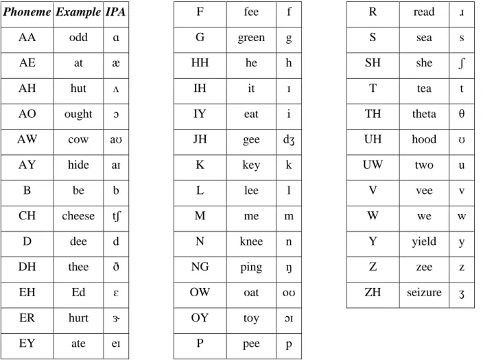
Given the alignments of the sound features (PLP values) and the phonemes they represent, we then trained GMMs on this more heavily labeled data. Instead of creating one model per accent, we had one model per phoneme, per accent. Table
21
4.3-2 lists the 39 phonemes in the American English language that we used, with an example of its pronunciation listed alongside each phoneme (in ARPABET6
notation). The IPA7 symbol is given as well. For our models, even though the
TextGrid files from the forced alignment process included silences, we ignored all silences and only used the 39 phonemes.
6 A phonetic transcription used by the Advanced Research Projects Agency (ARPA), more
importantly used in the CMU Pronunciation Dictionary.
7 International Phonetic Alphabet: phonetic notation based on the Latin alphabet, used to represent
22
Phoneme Example IPA
AA odd ɑ AE at æ AH hut ʌ AO ought ɔ AW cow aʊ AY hide aɪ B be b CH cheese tʃ D dee d DH thee ð EH Ed ɛ ER hurt ɝ EY ate eɪ F fee f G green g HH he h IH it ɪ IY eat i JH gee dʒ K key k L lee l M me m N knee n NG ping ŋ OW oat oʊ OY toy ɔɪ P pee p R read ɹ S sea s SH she ʃ T tea t TH theta θ UH hood ʊ UW two u V vee v W we w Y yield y Z zee z ZH seizure ʒ
Table 4.3-2: List of phonemes in ARPABET notation with an example in an English word, and in IPA notation
As parameters for each model, we tested solely with full covariance matrices (when we attempted to use tied, all 7 test sets of accents classified as only the 3 accents with the largest amount of data). We also tested with a varying number of mixtures, but on the linear order of single-digits (we would not need more than several distributions per model since each model is already very specific, unlike the models in the text-independent classifier). In order to evaluate these results, we reran the text-independent Classifier with the same subsets of accents from this text-dependent Classifier and compared the performances between the two.
Results for the 7-way classification are shown in Table 4.3-3 and Figure 4.3-1. Compared to the text-independent classifier using 128 mixtures in the first row, overall the text-dependent classifier performed about 3-4% higher, with higher
23
scores in every accent. It is the case that even though the overall performance peaked at 45.12% with 3 Gaussian mixtures, 2 mixtures maximized a high overall accuracy with relatively higher accuracies across each accent. We speculate that having 2 mixtures per phoneme was able to capture the middle segment and the outer segments of that phoneme. The spread of each accent’s accuracies in Figure 4.3-1 shows that with more components, the text-dependent classifier would eventually overfit to the larger available data.
For all following tables, numbers in bold represent the best accuracies per column, and the number of test files (representing 25% of that accent’s total files, according to the train-test split) are put in parentheses next to each accent’s column header. The sequence of accents across the row is in order from largest dataset (Hindi, with 87 test files) to smallest (Indonesian, with 24 test files). The same data is represented in graph format below each table.
Classifier Overall HI (87) FR (71) MA (70) KO (43) AR (28) CZ (25) IN (24) 128-untrans 41.38 58.62 47.89 55.71 30.23 14.29 8 4.17 1-trans 41.67 56.32 42.25 50 27.91 25 16 33.33 2-trans 44.54 59.77 49.3 61.43 32.56 17.86 8 16.67 3-trans 45.12 70.11 53.52 60 18.6 14.29 4 12.5 4-trans 43.68 74.71 56.34 52.86 13.95 7.14 0 8.33
Table 4.3-3: Percentage accuracies of all 7 accents where chance is 25% (proportion of HI files)
24
Figure 4.3-1: Graph of percentage accuracies of all 7 accents where chance is 25% (proportion of HI files)
Next we wanted to compare similar sized accents together. Table 4.3-4 corresponds with Figure 4.3-2, running the 128-component text-independent
classifier and the 2-component Transcribed classifier on the larger datasets (Hindi, French, and Mandarin). We can see that each accent performed equally well if not better on the text-dependent classifier over the text-independent classifier, with an overall improvement of 3.95%.
Classifier Overall HI (87) FR (71) MA (70)
128-untrans 61.4 66.67 50.7 65.71
2-trans 65.35 66.67 56.34 72.86
Table 4.3-4: Percentage accuracies of larger datasets, where chance is 36.36% (proportion of HI files)
25
Figure 4.3-2: Graph of percentage accuracies of larger datasets, where chance is 36.36% (proportion of HI files)
Looking at the results from the accents with less than 45 test files, namely Korean, Arabic, Czech, and Indonesian, the overall performance of the
text-dependent classifier was the same as the text-intext-dependent . Seen in Table 4.3-5 and Figure 4.3-3, Korean, Arabic and Czech yielded similarly worse results from the text-dependent classifier while Indonesian was identified much better through the phoneme-based models. Because the general spread of positive performance per accent is better in the text-dependent results, we have reason to believe that the text-dependent classifier is more robust.
26
Classifier Overall KO (43) AR (28) CZ (25) IN (24)
128-untrans 50 79.07 50 40 8.33
2-trans 50 69.77 46.43 32 37.5
Table 4.3-5: Percentage accuracies of smaller datasets, where chance is 35.83% (proportion of KO files)
Figure 4.3-3: Graph of percentage accuracies of smaller datasets, where chance is 35.83% (proportion of KO files)
Lastly, I considered sampling one accent per relative test size, and these three happened to be in the set of East Asian accents: Mandarin, Korean, and Indonesian. Unsurprisingly, Mandarin had higher accuracies than Korean and Indonesian, since it had the most data. But the text-dependent classifier
consistently held an improved performance for each accent as compared to its text-independent counterpart, as seen in Table 4.3-6 and Figure 4.3-4.
27
Classifier Overall MA (70) KO (43) IN (24)
128-untrans 52.55 75.71 37.21 12.5
2-trans 56.2 77.14 44.19 16.67
Table 4.3-6: Percentage accuracies of East Asian accent datasets, where chance is 51.09% (proportion of MA files)
Figure 4.3-4: Graph of percentage accuracies of East Asian accent datasets, where chance is 51.09% (proportion of MA files)
4.4 Confusion Matrices
The previous section showed percentage performances of the entire batch of test data for each of the seven accents. However, we wanted to examine if there were tendencies for certain accents to get confused with others. Using the set of three East Asian accents (Mandarin, Korean, and Indonesian) in the text-dependent classifier, we used the Confusion Matrix function of SciKit-Learn in order to see
28
how often each of our target accent’s test files were classified as each of the 7 possible accents. The results are given in Table 4.4-1.
Guess Actual Accent
MA (70) KO (43) IN (24) FR(71) 8.57% 9.30% 12.50% MA (70) 61.43% 37.21% 37.50% KO (43) 14.29% 32.56% 8.33% CZ (25) 0.00% 2.33% 0.00% AR (28) 5.71% 11.63% 4.17% HI (87) 8.57% 6.98% 20.83% IN (24) 1.43% 0.00% 16.67%
Table 4.4-1: Confusion Matrix of the Transcribed classifier for Mandarin, Korean, and Indonesian, displaying how often each set of files were guessed as the 7 possible
options.
We see that for Korean and Indonesian test files, a majority of them are classified as Mandarin (as opposed to Hindi which has more data), which implies that there must be an interaction between the acoustic phonetics of Mandarin and the other two Asian accents. Then for Mandarin, the second best guess after itself is to label a file as Korean 14.29% of the time. This also points to a possible interaction between Mandarin and Korean.
4.5 Phoneme Analysis
Beyond testing each file, we wanted to know if overall each phoneme was more or less being classified correctly. We collected data on each phoneme in each batch of test data for each accent, and calculated the total likelihood for the
29
phoneme across each occurrence. As predicted, a majority of phonemes in the larger data classified to the correct accent. For example, among the 39 phonemes in Hindi, only 2 of them are more often classified as non-Hindi accents. Even though Hindi had an overall 59.77% accuracy, the phoneme models were robust and accurate. To account for the discrepancy between good phoneme models and mis-classification of individual test files for Hindi, we can attribute the errors in actual testing to be from individual variations in the files. Further discussion of sources of error is given in sections 5.2 and 5.3.
30
5. Conclusion
5.1 Summary
We set out to replicate Choueiter et al.’s baseline (2008) that achieved a 23-way accent identification rate of 22% on the CSLU FAE corpus. We used PLP features to train GMMs without transcriptions, yet could only achieve 17.87% at best. Moving on to our second method, we acquired transcriptions of 7 sets of accents in order to train phoneme-specific models. The text-dependent classifier with 3 components outperformed the best text-independent classifier by a 7-way accent identification rate of 45.12% to 41.38% (a 3.74% difference). This margin was repeatedly found when testing on a subset of accents with larger data (HI, FR, and MA), a 3.95% difference, and on East Asian accents (MA, KO, and IN), a 3.65% difference – always favoring the text-dependent classifier. The equal overall
performance on the subset of accents with smaller data seemed puzzling at first, but this can be countered with the more even spread of accuracies for each accent for the phoneme-specific model than the text-independent version.
Additionally, similar to Angkititrakul and Hansen (2006), we found that accents whose languages are more related are more likely to be confused with each other, as seen in our results from the Mandarin and Korean confusion matrices.
The differences in data size proved to be causing some overfitting to the larger files, but overall we achieved the goal of building a phoneme-specific classifier that would perform better than a text-independent classifier.
5.2 Further Discussion
For the text-dependent classifier, Hindi—though the largest data set— required more components than 2 in order to outperform Mandarin. We speculate
31
that native Hindi speakers have generally migrated from a wide variety of locations. These immigrants from India often use Hindi in certain formal or schooling
situations and in parallel with their own local dialect or language, so this would increase the variation of speech. In contrast, Mandarin-speaking immigrants often come from a smaller set of regions of China and Taiwan such as Beijing, Shanghai, Taiwan, and Hong Kong. Mandarin is also more mainstreamed into their daily common speech, so the speakers in the Mandarin accent data set would have a more standardized accent.
While the independent classifier performed decently and the
text-dependent classifier performed better, plenty of errors were made in the prediction of these sound files. Some of these sources of error could be from the variation in heaviness of accent (e.g. how fluent speakers’ English is and when they immigrated to the United States), speaker-dependent vocal characteristics (i.e. gender and age), or dialect and country of origin (e.g. Arabic-speakers have their own dialect such as Syrian, Egyptian, Jordanian, etc.).
5.3 Future Work
Upon analysis, a number of factors could have gone into lowering the accuracies of our classifiers. As discussed in the previous section, three possible sources of error from the variability in speakers are gender, heaviness of accent, and dialect. If we could have labels for each sound file that marked these
characteristics, then we could manipulate gender, for example, as a constant
variable and test within female or within male subjects. It is noted that some of the files in the CSLU FAE corpus came with labels for these three traits, but they were not consistently labeled with the same metric. For example, most files’ labels said “general intelligibility: good” even when the levels of English proficiency varied greatly. For a full analysis, we should obtain labels for all files and use a
32
Furthermore, the measurement of acoustic features of the sound files could have been limiting in a couple of ways. Because these files were all telephone speech, the reduced bandwidth and extra noise in the background may have reduced the quality. We also only used PLP coefficients, which does not take into account pitch. In tonal languages like Mandarin, pitch and tone would have great influence and would carry over into speaking English. If we trained the GMMs with pitch as a factor, perhaps we could address the confusion between Mandarin and Korean and better differentiate them.
In terms of general classification techniques, we hope to experiment in the future with 5 specific improvements. First, when we built GMMs with increasing numbers of mixtures, they were initialized randomly. However, a smarter way of training models would be to do successive state splitting (Takami and Sagayama, 1992). This is a common method used in speech recognition that starts with 1 mixture, then optimally splits into 2, then 4, etc. Next, if we had the computational time and space, we would like to perform n-fold cross-validation, a statistical
technique that would iterate over multiple different splits of train-test data. Thirdly, interpolation between our phone-specific and text-independent classifiers could have produced more robust results, especially given that some accents with less data had less phonemes. Interpolation would let us calculate a weighted
combination of both sets of models, which could be in favor of our smaller datasets. The last set of techniques we thought about implementing are related to the phonemes themselves. If we could isolate and focus on the English phonemes that are typologically more marked (or less common in the world) such as /ER/, perhaps our models would better capture the accent-specific characteristics of non-native speakers saying /ER/ differently. Another step that would further reduce the size of phonemes and make the feature space concise is to take out low-energy consonants like stops and fricatives. This was said to aid in speaker recognition, according to Angkititrakul and Hansen (2006).
Aside from improving the classifier itself, we had originally hoped to build a publicly available web application out of these systems. Users would be able to
33
record themselves saying a specific piece of text, and our application would force-align the speech in real-time, then use the already trained GMMs to classify their speech as one of the trained accents. This would have involved a significant amount of front-end development, and unfortunately time proved to be a limiting factor.
34
References
Angkititrakul, P., & Hansen, J. H. (2006). Advances in phone-based modeling for
automatic accent classification. Audio, Speech, and Language Processing, IEEE Transactions on, 14(2), 634-646.
Chen, N. F., Shen, W., & Campbell, J. P. (2010). A linguistically-informative approach to dialect recognition using dialect-discriminating context-dependent phonetic models. In Acoustics Speech and Signal Processing (ICASSP), 2010 IEEE International Conference on (pp. 5014-5017). IEEE. Choueiter, G., Zweig, G., & Nguyen, P. (2008). An empirical study of automatic
accent classification. In Acoustics, Speech and Signal Processing, 2008. ICASSP 2008. IEEE International Conference on (pp. 4265-4268). IEEE. “CSLU foreign-accented english corpus,” http://www.cslu.ogi.edu/corpora/fae/. Ge, Z. (2016). Improved Accent Classification Combining Phonetic Vowels with
Acoustic Features. arXiv preprint arXiv:1602.07394.
Parent, G., & Eskenazi, M. (2010). Toward better crowdsourced transcription:
Transcription of a year of the let's go bus information system data. In Spoken Language Technology Workshop (SLT), 2010 IEEE (pp. 312-317). IEEE. Reddy, S., & Stanford, J. (2015). Toward completely automated vowel extraction:
Introducing DARLA. Linguistics Vanguard.
Reynolds, D. A., & Rose, R. C. (1995). Robust text-independent speaker
identification using Gaussian mixture speaker models. Speech and Audio Processing, IEEE Transactions on, 3(1), 72-83.
Sangwan, A., & Hansen, J.H. (2012). "Automatic Analysis of Mandarin Accented English Using Phonological Features." Speech Communication 54.1, 40-54. Takami, J. I., & Sagayama, S. (1992). A successive state splitting algorithm for
efficient allophone modeling. In Acoustics, Speech, and Signal Processing, 1992. ICASSP-92., 1992 IEEE International Conference on (Vol. 1, pp. 573-576). IEEE.
35
Woodland, P. C., Gales, M. J. F., Pye, D., & Young, S. J. (1997). The development of the 1996 HTK broadcast news transcription system. In DARPA speech
recognition workshop (pp. 73-78). Morgan Kaufmann Pub.
Young, S. J., & Young, S. (1993). The HTK hidden Markov model toolkit: Design and philosophy (p. 28). University of Cambridge, Department of Engineering. Yuan, J., & Liberman, M. (2008). Speaker identification on the SCOTUS corpus.