Summer 7-9-2015
Boa: Ultra-Large-Scale Software Repository and
Source Code Mining
Robert Dyer
Bowling Green State University, rdyer@bgsu.edu
Hoan Anh Nguyen
Iowa State University, hoan@iastate.edu
Hridesh Rajan
Iowa State University, hridesh@iastate.edu
Tien N. Nguyen
Iowa State University, tien@iastate.edu
Follow this and additional works at:
http://lib.dr.iastate.edu/cs_techreports
Part of the
Programming Languages and Compilers Commons
, and the
Software Engineering
Commons
This Article is brought to you for free and open access by the Computer Science at Iowa State University Digital Repository. It has been accepted for inclusion in Computer Science Technical Reports by an authorized administrator of Iowa State University Digital Repository. For more information,
Recommended Citation
Dyer, Robert; Nguyen, Hoan Anh; Rajan, Hridesh; and Nguyen, Tien N., "Boa: Ultra-Large-Scale Software Repository and Source Code Mining" (2015).Computer Science Technical Reports. 374.
Boa: Ultra-Large-Scale Software Repository and Source Code Mining
AbstractIn today’s software-centric world, ultra-large-scale software repositories, e.g. SourceForge, GitHub, and
Google Code, are the new library of Alexandria. They contain an enormous corpus of software and related
information. Scientists and engineers alike are interested in analyzing this wealth of information. However,
systematic extraction and analysis of relevant data from these repositories for testing hypotheses is hard, and
best left for mining software repository (MSR) experts! Specifically, mining source code yields significant
insights into software development artifacts and processes. Unfortunately, mining source code at a large-scale
remains a difficult task. Previous approaches had to either limit the scope of the projects studied, limit the
scope of the mining task to be more coarse-grained, or sacrifice studying the history of the code. In this paper
we address mining source code: a) at a very large scale; b) at a fine-grained level of detail; and c) with full
history information. To address these challenges, we present domain-specific language features for source
code mining in our language and infrastructure called Boa. The goal of Boa is to ease testing MSR-related
hypotheses. Our evaluation demonstrates that Boa substantially reduces programming efforts, thus lowering
the barrier to entry. We also show drastic improvements in scalability.
Keywords
mining, software, repository, scalable, ease of use, lower barrier to entry, Boa, domain-specific languages
DisciplinesBoa: Ultra-Large-Scale Software Repository and Source Code Mining
ROBERT DYER, Bowling Green State University
HOAN ANH NGUYEN, Iowa State University
HRIDESH RAJAN, Iowa State University
TIEN N. NGUYEN, Iowa State University
In today’s software-centric world, ultra-large-scale software repositories, e.g. SourceForge, GitHub, and Google Code, are the new library of Alexandria. They contain an enormous corpus of software and related information. Scientists and engineers alike are interested in analyzing this wealth of information. However, systematic extraction and analysis of relevant data from these repositories for testing hypotheses is hard, and best left for mining software repository (MSR) experts! Specifically, mining source code yields significant insights into software development artifacts and processes. Unfortunately, mining source code at a large-scale remains a difficult task. Previous approaches had to either limit the scope of the projects studied, limit the scope of the mining task to be more coarse-grained, or sacrifice studying the history of the code. In this paper we address mining source code: a) at a very large scale; b) at a fine-grained level of detail; and c) with full history information. To address these challenges, we present domain-specific language features for source code mining in our language and infrastructure calledBoa. The goal ofBoais to ease testing MSR-related hypotheses. Our evaluation demonstrates that
Boasubstantially reduces programming efforts, thus lowering the barrier to entry. We also show drastic improvements in scalability.
CCS Concepts:•Software and its engineering→Distributed programming languages;
Additional Key Words and Phrases: mining; software; repository; scalable; ease of use; lower barrier to entry
ACM Reference Format:
Robert Dyer, Hoan Anh Nguyen, Hridesh Rajan, and Tien N. Nguyen, 2015. Boa: Ultra-Large-Scale Software Repository and Source Code Mining.ACM Trans. Softw. Eng. Methodol.1, 1, Article 1 (July 2015), 33 pages.
DOI:0000001.0000001
1. INTRODUCTION
Ultra-large-scale software repositories, e.g. SourceForge (330,000+ projects), GitHub (250,000+ projects), and Google Code (250,000+ projects) contain an enormous collection of software and information about software. Assuming only a meager 1K lines of code (LOC) per project, these big-3 repositories amount to at least 8.61 billion LOC alone. Scientists and engineers alike are interested in analyzing this wealth of information both for curiosity as well as for testing such important hypotheses as:
— “how people perceive and consider the potential impacts of their own and others’ edits as they write together? [Dourish and Bellotti 1992]”;
— “what is the most widely used open source license? [Lerner and Tirole 2002]”;
The work described in this article is the revised and extended version of articles in the proceedings of the 35th International Conference on Software Engineering (ICSE’13) [Dyer et al. 2013] and the 12th International Conference on Generative Programming: Concepts & Experiences (GPCE’13) [Dyer et al. 2013b].
Author’s addresses: R. Dyer, Department of Computer Science, Bowling Green State University; H. Rajan, Department of Computer Science, Iowa State University; H. Nguyen and T. Nguyen, Department of Electrical and Computer Engineering, Iowa State University.
This work was supported in part by the US National Science Foundation (NSF) under grants CNS-15-13263, CNS-15-12947, CCF-14-23370, CCF-13-49153, CCF-13-20578, TWC-12-23828, CCF-11-17937, CCF-10-17334, and CCF-10-18600. Permission to make digital or hard copies of all or part of this work for personal or classroom use is granted without fee provided that copies are not made or distributed for profit or commercial advantage and that copies bear this notice and the full citation on the first page. Copyrights for components of this work owned by others than ACM must be honored. Abstracting with credit is permitted. To copy otherwise, or republish, to post on servers or to redistribute to lists, requires prior specific permission and/or a fee. Request permissions from permissions@acm.org.
c
2015 ACM. 1049-331X/2015/07-ART1 $15.00
— “how many projects continue to use DES (considered insecure) encryption standards? [Landau 2000]”;
— “how many open source projects have a restricted export control policy? [Goodman et al. 1995]”; — “how many projects on an average start with an existing code base from another project instead of
scratch? [Raymond 1999]”;
— “how often do practitioners use dynamic features of JavaScript, e.g. eval? [Richards et al. 2011]”; and
— “what is the average time to resolve a bug reported as critical? [Weiss et al. 2007]”.
However, the current barrier to entry could be prohibitive. For example, to answer the questions above, a research team would need to (a) develop expertise in programmatically accessing version control systems, (b) establish an infrastructure for downloading and storing the data from software repositories since running experiments by directly accessing this data is often time prohibitive, (c) program an infrastructure in a full-fledged programming language like C++, Java, C#, or Python to access this local data and answer the hypothesis, and (d) improve the scalability of the analysis infrastructure to be able to process ultra-large-scale data in a reasonable time.
These four requirements substantially increase the cost of scientific research. There are four ad-ditional problems. First, experiments are often not replicable because replicating an experimental setup requires a mammoth effort. Second, reusability of experimental infrastructure is typically low because analysis infrastructure is not designed in a reusable manner. After all, the focus of the orig-inal researcher is on the result of the analysis and not on reusability of the analysis infrastructure. Thus, researchers commonly have to replicate each other’s efforts. Third, data associated and pro-duced by such experiments is often lost and becomes inaccessible and obsolete [González-Barahona and Robles 2012], because there is no systematic curation. Last but not least, building analysis in-frastructure to process ultra-large-scale data efficiently can be very hard [Dean and Ghemawat 2004; Pike et al. 2005; Chambers et al. 2010].
To solve these problems, we designed a domain-specific programming language for analyzing ultra-large-scale software repositories, which we callBoa. In a nutshell, Boaaims to be for open source-related research what Mathematica is to numerical computing, R is for statistical computing, and Verilog and VHDL are for hardware description. We have implemented Boaand provide a web-based interface toBoa’s infrastructure [Rajan et al. 2014]. Potential users request access to the system and are typically granted it within a few hours or days. Our eventual goal is to open-source all of theBoainfrastructure.
Boaprovides domaspecific language features for mining source code. These features are in-spired by the rich body of literature on object-oriented visitor patterns [Gamma et al. 1994; Hie 2012; Oliveira et al. 2008; Orleans and Lieberherr 2001; Visser 2001]. A key difference from previ-ous work is that we do not require the host language to contain object-oriented features. Ourvisitor typesprovide a default depth-first search (DFS) traversal strategy, while still maintaining the flexi-bility to allow custom traversal strategies. Visitor types allow specifying the behavior that executes for a given node type,beforeoraftervisiting the node’s children.Boaalso provides abstractions for dealing with mining of source code history, such as the ability to retrieve specific snapshots based on date. We also show several useful patterns for source code mining that utilize these domain specific language features.
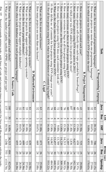
To evaluateBoa’s design and effectiveness of its infrastructure we wrote programs to answer 23 different research questions in five different categories: questions related to the use of programming languages, project management, legal, platform/environment, and source code. Our results show thatBoasubstantially decreases the efforts of researchers analyzing human and technical aspects of open source software development allowing them to focus on their essential tasks. We also see ease of use, substantial improvements in scalability, and lower complexity and size of analysis programs (see Figure 12). Last but not least, replicating an experiment conducted usingBoais just a matter of re-running, often small,Boaprograms provided by previous researchers.
We now describeBoaand explore its advantages. First, we further motivate the need for a new language and infrastructure to perform software mining at an ultra-large scale. Next we present the language (Section 3) and describe its infrastructure (Section 4). Section 5 presents studies of applicability and scalability. Section 7 positions our work in the broader research area and Section 8 concludes.
2. MOTIVATION
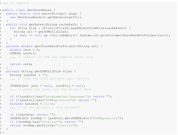
Creating experimental infrastructure to analyze the wealth of information available in open source repositories is difficult [Bevan et al. 2005; Promise dataset 2009; González-Barahona and Robles 2012; Shang et al. 2010; Gabel and Su 2010]. Creating an infrastructure that scales well is even harder [Shang et al. 2010; Gabel and Su 2010]. To illustrate, consider a question such as “what are the average numbers of changed files per revision (churn rates) for all Java projects that use SVN?” Answering this question would require knowledge of (at a minimum): reading project metadata and mining code repository locations, how to access those code repositories, additional filtering code, controller logic, etc. Writing such a program in Java for example, would take upwards of 70 lines of code and require knowledge of at least 2 complex libraries. A heavily elided example of such a program is shown in Figure 1.
1... // imports
9public class GetChurnRates {
10 public static void main(String[] args) { 11 new GetChurnRates().getRates(args[0]); 12 }
13 public void getRates(String cachePath) {
14 for (File file : (File[])FileIO.readObjectFromFile(cachePath)) { 15 String url = getSVNUrl(file);
16 if (url != null && !url.isEmpty()) System.out.println(getChurnRateForProject(url));
17 }
18 }
19 private double getChurnRateForProject(String url) { 20 double rate = 0;
21 SVNURL svnUrl;
22 ... // connect to SVN and compute churn rate 36 return rate;
37 }
38 private String getSVNUrl(File file) { 39 String jsonTxt = "";
40 ... // read the file contents into jsonTxt 49 JSONObject json = null, jsonProj = null; 50 ... // parse the text, get the project data
56 if (!jsonProj.has("programming-languages")) return ""; 57 if (!jsonProj.has("SVNRepository")) return ""; 58 boolean hasJava = false;
59 ... // is the project a Java project? 63 if (!hasJava) return "";
64 JSONObject svnRep = jsonProj.getJSONObject("SVNRepository"); 65 if (!svnRep.has("location")) return "";
66 return svnRep.getString("location"); 67 }
68 }
Fig. 1. Java program that answers the question “what are the churn rates for all Java projects that use SVN?” This program assumes that the user has manually downloaded all project metadata, available as JSON files, and SVN repositories from SourceForge, a forge for making open-source projects available [SourceForge 2014]. It then processes the data using a JSON library and collects a list of
Subversion URLs. A SVN library is then used to connect to each cached repository in that list and calculate the churn rate for the project. Notice that this code required use of 2 complex, external libraries in addition to standard Java classes and resulted in almost 70 lines of code. It is also sequential, so it will not scale as the data size grows. One could write a concurrent version, but this would add complexity.
2.1. Boa: Enabling Data Intensive Open Source Research
We designed and implemented a domain-specific programming language that we callBoato solve these problems.Boaaims to lower the barrier to entry and thus enable a larger, more ambitious line of data intensive scientific discovery in open source software development-related research. The main features ofBoaare inspired from existing languages for data-intensive computing [Dean and Ghemawat 2004; Pike et al. 2005; Olston et al. 2008; Isard et al. 2007]. To these we add built-in types that are specifically designed to ease analysis tasks common in open source software mining research.
To illustrate the features of Boa, consider the same question “what are the churn rates for all Java projects that use SVN?”. A Boaprogram to answer this question is shown in Figure 2. On line 1, this program declares an output calledrates, which collects integer values and produces a final result by aggregating the input values for each project (indexed by a string) using the function mean. On line 2, it declares that the input to this program will be a project, e.g. Apache OpenOffice. Boa’s infrastructure manages the details of downloading projects and their associated information. For each project, the code on lines 3–6 runs. If a repository contains 700k projects, the code on lines 3–6 runs for each.
1rates: output mean[string] of int; 2p: Project = input;
3foreach (i: int; p.code_repositories[i].kind == RepositoryKind.SVN
&& len(p.code_repositories[i].revisions) > 10) 4 exists (j: int; lowercase(p.programming_languages[j]) == "java")
5 foreach (k: int; len(p.code_repositories[i].revisions[k].files) < 100) 6 rates[p.id] << len(p.code_repositories[i].revisions[k].files);
Fig. 2. Boa program that answers the question “what are the churn rates for all Java projects that use SVN?”
On line 3, this program says to run code on lines 4–6 for each of the input project’s code reposi-tories that are Subversion and contain more than 10 revisions (to filter out new or toy projects). On line 4, this program says to run code on lines 5–6, if and only if for the input project at least one of the programming languages used is Java. Line 5 selects only revisions from such repositories that have less than 100 files changed (to filter out extremely large commits, such as the first commit of a project). Finally, on line 6, this program says to send the length of the array that contains the changed files in the revision to the aggregator rates, indexed by the project’s unique identifier string. This aggregator produces the final answer to our question.
These 6 lines of code not only answer the question of interest, but run on a distributed cluster po-tentially saving hours of execution time. Note that writing this small program required no intimate knowledge of how to find/access the project metadata, how to access the repository information, or any mention of parallelization. All of these concepts are abstracted from the user, providing instead simple primitives such as theProjecttype which contains attributes related to software projects such as the name, programming languages used, repository locations, etc. These abstractions sub-stantially ease common analysis tasks.
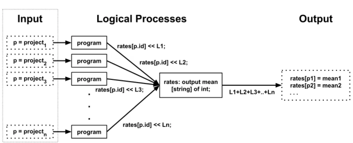
Figure 3 shows an example of the semantic model provided byBoa. On the left-hand side, each project from the dataset becomes a single input to a process. The program is instantiated once for each input (middle of figure). Each instantiation will process a single project, computing the churn rate for that one project. For each revision in the project, the number of files in that revision is sent
p = project 1 p = project 2 p = project 3 p = project n
.
.
.
program program program program.
.
.
rates: output mean [string] of int;
rates[p1] = mean1 rates[p2] = mean2 . . .
rates[p.id] << L1;
Input
Logical Processes
Output
L1+L2+L3+..+Ln rates[p.id] << Ln;
rates[p.id] << L2; rates[p.id] << L3;
Fig. 3. Overview of the semantic model provided byBoafor the query in Figure 2. Each project is a single input and fed to a single process. Each process sends messages to the output process. The output process produces the final result. Each solid box represents a logical process.
7,000 70,000 700,000 1 10 100 1,000 10,000 100,000 13 424 10,409 15 17 22 Java Boa
Input Size (number of projects)
T im e ( s e c ) 473x speedup
Fig. 4. Performance results for programs in Figures 1 and 2.
to the output process (right-hand side) which aggregates all the values, from each input process, and computes the final result.
Since this program runs on a cluster, it also scales extremely well compared to the (sequential) version written in Java. The time taken to run this program on varying input sizes is shown in the lower right of Figure 4. Note that the y-axis is in logarithmic scale. The time to execute the Java program increases roughly linearly with the size of the input while theBoaprogram sees minimal increase in execution time.
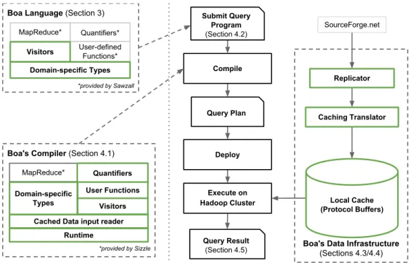
We have built an infrastructure for theBoaprogramming language. An overview of this infras-tructure is presented in Figure 5. Components are shown inside dotted boxes on the left, the flow of aBoaprogram is shown in the middle, and the input data sources are shown on the right.
The three main components are: theBoalanguage, compiler and runtime, and supporting data in-frastructure. First, an analysis task is phrased as aBoaprogram, e.g. that in Figure 2 (see Section 3). This program is fed to our compiler (see Section 4.1) via our web-based interface (see Section 4.2). The Boacompiler produces a query plan. Our infrastructure then deploys this query plan onto a Hadoop [Apache Software Foundation 2014a] cluster, where it executes. The cluster makes use of a locally cached copy of the source code repositories (see Sections 4.3–4.4) and based on the query
Boa's Data Infrastructure (Sections 4.3/4.4) Local Cache (Protocol Buffers) Replicator Caching Translator SourceForge.net Compile Execute on Hadoop Cluster Deploy Submit Query Program (Section 4.2) Query Plan Query Result (Section 4.5) Boa's Compiler (Section 4.1)
*provided by Sizzle
MapReduce*
Domain-specific Types
Quantifiers
Cached Data input reader Visitors User Functions
Runtime
Quantifiers* Boa Language (Section 3)
*provided by Sawzall MapReduce* User-defined Functions* Visitors Domain-specific Types
Fig. 5. An Overview ofBoa’s Infrastructure. New components are marked with green boxes and bold text.
plan creates tasks to produce the final query result (see Section 4.5). This is the answer to the user’s analysis task. We now describe these components in detail.
3. DESIGN OF THEBOALANGUAGE
The top left portion of Figure 5 shows the main features of theBoalanguage. We have five main kinds of features at the moment: domain-specific types to ease analysis of open source software repository mining, declarative visitors to ease source code mining, MapReduce [Dean and Ghe-mawat 2004] support for scalable analysis of ultra-large-scale repositories, quantifiers for easily expressing loops, and the ability to define functions.
3.1. Domain-Specific Types inBoa
TheBoalanguage provides several domain-specific types for mining software repositories. Figure 6 gives an overview of these types. Each type provides several attributes that can be thought of as read-only fields.
Type Attributes
Project id, name, created_date, code_repositories, . . . CodeRepository url, kind, revisions
Revision id, log, committer, commit_date, files
ChangedFile name, kind, change
Person username, real_name, email
TheProjecttype provides metadata about an open source project in the repository, including its name, url, some descriptions, who maintains and develops it, and any code repository. This type is used as input to programs in theBoalanguage.
TheCodeRepositorytype provides all of theRevisions committed into that repository. A revision represents a group of artifact changes and provides relevant information such as the revi-sion id, commit log and time, thePersonwho committed the revision, and theChangedFiles committed.
Type Attributes
ASTRoot imports, namespaces
Namespace name, modifiers, declarations
Declaration name, kind, modifiers, parents, fields, methods, . . .
Type name, kind
Method name, modifiers, return_type, statements, . . . Variable name, modifiers, initializer, variable_type Statement kind, condition, expression, statements, . . . Expression kind, literal, method, is_postfix, . . . Modifier kind, visibility, other, . . .
Fig. 7. Domain-specific types for mining source code.
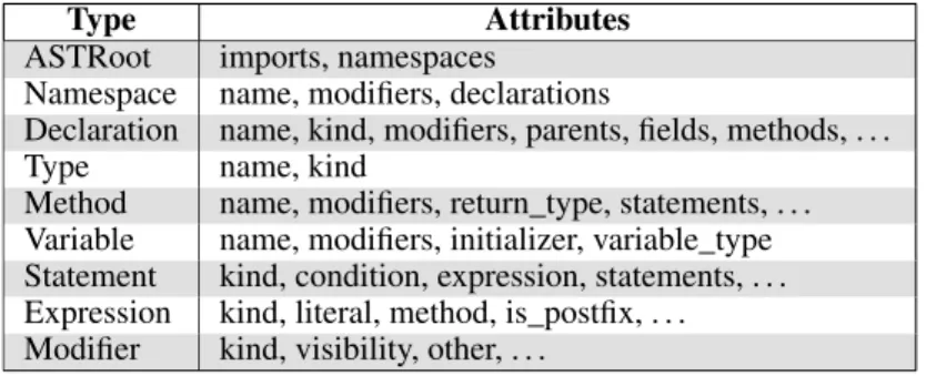
The types Boa provides for representing source code are shown in Figure 7 and
in-clude: ASTRoot, Namespace, Declaration, Method, Variable, Type, Statement,
Expression, andModifier. The declaration, type, statement, expression, and modifier types are discriminated types, meaning they actually represent the union of different record structures.
For example, consider the typeStatement. This type has an attributekind, which is an enu-merated value. Based on the kind of statement, specific additional attributes in the record will be set. For example, if the kind isTYPEDECLthen thetype_declattribute is defined. However if the kind isCATCHthen thetype_declis undefined.
Representing these types as discriminated types allowsBoato keep the number of types as small as possible. This makes supporting future languages easier by only needing to provide a mapping from the new language to the small set of types inBoa. Existing mining tasks would immediately be able to mine source code from the new language.
3.1.1. Mapping Java to Boa’s Custom AST. Currently, we have fully mapped the Java language toBoa’s schema, attempting to simplify the schema as much as possible. This gives a simple, yet flexible, schema capable of supporting the entire Java language (through Java 7). This allowsBoato represent Java source files in the dataset and allowsBoaprograms to query those Java source files.
The top-level symbol in Java’s grammar is aCompilationUnit. InBoa, the top-level type for source code isASTRoot. For each JavaCompilationUnit, we create oneASTRoot. The im-ports from theCompilationUnitdirectly map to the imports attribute inASTRoot. Everything between the import keyword and the semicolon is stored as a single string in the imports array. We then create oneNamespacetype inBoa, which contains thePackageName(or an empty string if the default package) and any modifiers.
Next, each Java type is transformed into a Declaration. The declaration’s kindattribute indicates if the type was a class, interface, enum, annotation, etc. Methods are transformed into Methods and fields transformed intoVariables. Finally each statement and expression are trans-formed.
3.1.2. Extending the AST to Support New Language Features.WhileBoakeeps these types as simple as possible, they are still flexible enough to support more complex language features. As
additional support for other source languages is added, if the schema is not capable of directly sup-porting a particular language feature theStatementKindorExpressionKindenumerations can be easily extended. For example, consider the enhanced-for loop in Java:
1for (String s : iter) 2 body;
which says to iterate over the expressioniterand for each string values, run thebody.Boa’s types do not directly contain anENHANCEDFORkind for this language feature.
Despite this design decision, an enhanced-for statement can be easily represented inBoa’s schema without having to extend it. First,Boagenerates aStatementof kindFOR. Inside that statement, Boasetsexpressiontoiter.Boaalso sets thevariable_declarationforString s in the statement. Thus, if a statement of kindFORhas itsvariable_declarationattribute set it is a for-each statement. If that attribute is not defined, then it is a standard for-loop.
Using a similar strategy, we plan to support additional languages. If we are unable to map a partic-ular language feature to the existing types and kinds, we can extend them. For example, supporting a null coalescing operator in C# would require extending the ExpressionKind with a new kind. Ex-tending the enumeration is backwards compatible, so previous mining tasks will continue to work as expected.
3.2. Declarative Visitors to Ease Source Code Mining
Users must be able to easily express source code mining tasks. For users who are intimately famil-iar with compilers and interpreters, the visitor style is well understood. However, other users may find two aspects of visitor-style traversals daunting. First, it generally requires writing a significant amount of boiler-plate code whose length is proportional to the complexity of the programming language being visited. Second, this strategy requires intimate familiarity with the structure of that programming language.
To make source code mining more accessible to all users, we investigated the design of more declarative features for mining source code. In this section, we describe our proposed syntax for writing source code mining tasks. The syntax was inspired by previous language features, such as the before and after visit methods in DJ [Orleans and Lieberherr 2001] and case expressions in Haskell [Jones 2003].
visitor::=visitor{visitClause*}
visitClause::=beforeClause|afterClause
beforeClause::=beforetypeList->beforeClauseStmt
afterClause::=aftertypeList->stmt
typeList::=_|identifier:type|type(,type)*
beforeClauseStmt::=stmt|stopStmt|visit(identifier) ;
stopStmt::=stop;
Fig. 8. Proposed syntax for easing source code mining.
The new syntax is shown in Figure 8. The top-level syntax for a mining task is avisitor type. Visitor types take zero or more visit clauses. A visit clause can be abefore or an after clause. During traversal of the tree, a before clause is executed when visiting a node of the specified type. If the default traversal strategy is used, then the node’s children will be visited. After all the children are visited, any matching after clause executes.
Before and after clauses take atype list. A type list can be a single type with an optional identifier, a list of types, or an underscore wildcard. The underscore wildcard provides default behavior for a visitor clause. This default executes for a node of type T if no other clause specifies T in its type list. Thus, the following code:
1id := visitor {
2 before Project, CodeRepository, Revision -> { } 3 before _ -> counter++;
4};
will execute the clause’s body on line 2 when traversing nodes of type Project,
CodeRepository, orRevision. When traversing a node of any other type, the default clause’s body on line 3 executes. The result of this code is thus a count of all nodes, excluding those of the types listed. Thus we count only the source code AST nodes for a project.
Note that unlike pattern matching and case expressions in functional languages like Haskell, the order of the before and after clauses do not matter. A type may appear in at most one before clause and at most one after clause.
To begin a mining task, users write avisitstatement:
visit(n, v);
that has two parts: the node to visit and a visitor. When this statement executes, a traversal starts at the node represented bynusing visitorv.
3.2.1. Supporting Custom Traversals.To allow users the ability to override the default traversal strategy, two additional statements are provided insidebeforeclauses. The first is thestop state-ment:
stop;
which when executed will stop the visitor from traversing the children of the current node. This is useful in cases where the mining task never needs to visit specific types further down the tree, allowing to stop at a certain depth. Note that stop acts similar to a return, so no statements after it are reachable.
If the default traversal is stopped, users may provide a custom traversal of the children with avisit statement:
visit(child);
which says to visit the node’schildtree once. This statement can be called on any subset of the children and in any order. This also allows for visiting a child more than once, if needed.
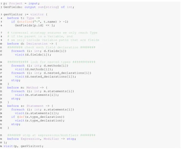
Figure 9 illustrates a custom traversal strategy from one of our case studies [Dyer et al. 2014]. This program answers the questionhow many fields that use a generic type parameter are declared in each project?To answer this question, the program declares a single visitor. This visitor looks for Typenodes where the name contains a generic type parameter (line 5). This visit clause by itself is not sufficient to answer the question, as generic type parameters might occur in other locations, such as the declaration of a class/interface, method parameters, locals, etc. Instead, a custom traversal strategy (lines 10–34) is needed to ensure only field declarations are included.
The traversal strategy first ensures all fields ofDeclarationare visited (lines 12–13). Since declarations can be nested (e.g. in Java, inside other types and in method declarations) we also must manually traverse to find nested declarations (lines 15–32). Finally, we don’t want to visit nodes of typeExpressionorModifier(line 34), as these node types can’t possibly contain a field declaration but may contain aTypenode.
Complex mining tasks can be simplified by using multiple visitors. For example, perhaps we only want to look for certain expressions inside of an if statement’s condition. We can write a visitor to find if statements, and then use a second sub-visitor to look for the specific expression by visiting the if statement’s children. We could perform this mining task with one visitor, however then we need to have flags set to track if we are in the tree underneath an if statement. Using multiple visitors keeps these two mining tasks separate and avoids using flags to keep it simple.
3.2.2. Mining Snapshots in Time.While our infrastructure contains data for the full revision his-tory of each file, some mining tasks may wish to operate on a single snapshot. We provide several helper functions to ease this use case. For example, the function:
1p: Project = input;
2GenFields: output sum[string] of int;
3genVisitor := visitor { 4 before t: Type ->
5 if (strfind("<", t.name) > -1) 6 GenFields[p.id] << 1;
7 # traversal strategy ensures we only reach Type 8 # if the parent is a Variable, and
9 # we only include Variable paths that are fields 10 before d: Declaration -> {
11 ######## check each field declaration ######## 12 foreach (i: int; d.fields[i])
13 visit(d.fields[i]);
14 ########### look for nested types ############ 15 foreach (i: int; d.methods[i])
16 visit(d.methods[i]);
17 foreach (i: int; d.nested_declarations[i]) 18 visit(d.nested_declarations[i]); 19 stop;
20 }
21 before m: Method -> {
22 foreach (i: int; m.statements[i]) 23 visit(m.statements[i]); 24 stop;
25 }
26 before s: Statement -> {
27 foreach (i: int; s.statements[i]) 28 visit(s.statements[i]); 29 if (def(s.type_declaration)) 30 visit(s.type_declaration); 31 stop; 32 } 33 ####### stop at expressions/modifiers ######## 34 before Expression, Modifier -> stop;
35 };
36 visit(p, genVisitor);
Fig. 9. Using a custom traversal strategy to find uses of generics in field declarations.
getsnapshot(CodeRepository [, time] [, string...])
takes aCodeRepositoryas its first argument. It optionally takes a time argument, specifying the time of the snapshot which defaults to the last time in the repository. The function also optionally takes a list of strings. If provided, these strings are used to filter files while generating the snapshot. The file’s kind is checked to see if it matches at least one of the patterns specified. For example:
getsnapshot(CodeRepository, "SOURCE_JAVA_JLS")
says to get the latest snapshot and filter any file that is not a valid Java source file.
A useful pattern is to write a visitor with a before clause forCodeRepositorythat gets a specific snapshot, visits the nodes in the snapshot, and then stops the default traversal:
1visitor {
2 before n: CodeRepository -> { 3 snapshot := getsnapshot(n); 4 foreach (i: int; def(snapshot[i])) 5 visit(snapshot[i]);
6 stop; 7 } 8 ... 9}
This visitor will visit all code repositories for a project, obtain the last snapshot of the files in that repository, and then visit the source code of those files. This pattern is useful for mining thecurrent versionof a software repository.
3.2.3. Mining Revision Pairs. Often a mining task might want to locate certain revisions and com-pare files at that revision to their previous state. For example, our motivating example looks for revisions that fixed bugs and then compares the files at that revision to their previous snapshot. To accomplish this task, one can use the following pattern:
1files: map[string] of ChangedFile;
2v := visitor {
3 before f: ChangedFile -> { 4 if (def(files[f.name])) {
5 ... # task comparing f and files[f.name]
6 }
7 files[f.name] = f; 8 }
9};
which declares a map of files, indexed by their path. The code on line 4 checks if a previous version of the file was cached. If it was, the code on line 5 executes wherefrefers to the current version of the file being visited and the expressionfiles[f.name]refers to the previous version of the file. Finally, the code on line 7 updates the map, storing the current version of the file.
3.2.4. Bringing It All Together.Consider the hypothesis “a large number of bug fixes add checks fornull”. In this section, we describe a solution to support that hypothesis.
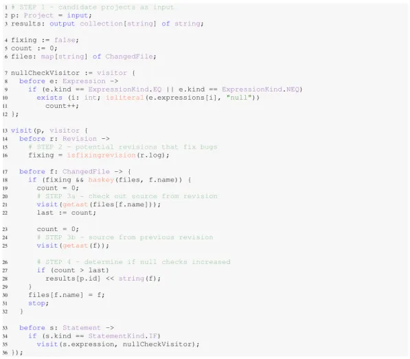
Consider the Boa program in Figure 10, which implements the entire mining task. This pro-gram takes a single project as input. It then passes the propro-gram’s data tree to a visitor (line 13). This visitor keeps track if the lastRevisionseen was a fixing revision (line 16). When it sees a ChangedFileit looks at the current revision’s log message and if it is a fixing revision it will get snapshots of the current file and the previous version of the file and visit their AST nodes (lines 21 and 25).
When visiting the AST nodes for these snapshots, if it encounters a Statementof kindIF (line 34), it then uses a sub-visitor to check if the statement’s expression contains a null check (lines 35 and 7–12) and increments a counter (line 11). Thus we will know the number of null checks in each snapshot and can compare (line 27) to see if there are more null checks. Note that this analysis is conservative and may not find all fixing revisions that add null checks, as the revision may also removea null check from another location and thus give the same count.
This task illustrates several features mentioned earlier in this section. First, the second visitor shows use of a custom traversal strategy by utilizing a stop statement. Second, it makes use of a sub-visitor (nullCheckVisitor). Third, it uses the revision pair pattern to check several versions of a file.
Finally, writing this task required no explicit mention of parallelizing the query. Writing the same task in Hadoop would require a lot of boilerplate code to manually parallelize the task, whereas the Boa version is automatically parallelized.
3.3. MapReduce Support inBoa
In MapReduce [Dean and Ghemawat 2004] frameworks, computations are specified via two user-defined functions: a mapperthat takes key-value pairs as input and produces key-value pairs as output, and areducerthat consumes those key-value pairs and aggregates data based on individ-ual keys. Syntactically,Boais reminiscent of Sawzall [Pike et al. 2005], a language designed for analyzing log files. InBoa, like Sawzall, users write the mapper functions directly and use built-in aggregators as the reduce function. Users declare output variables, process the input, and then send values to the tables. Output declarations specify aggregation functions and the language provides several built in aggregators, such as sum, minimum/maximum, mean, etc.
1# STEP 1 - candidate projects as input 2p: Project = input;
3results: output collection[string] ofstring;
4fixing := false; 5count := 0;
6files: map[string] of ChangedFile;
7nullCheckVisitor := visitor { 8 before e: Expression ->
9 if (e.kind == ExpressionKind.EQ || e.kind == ExpressionKind.NEQ) 10 exists (i: int; isliteral(e.expressions[i], "null"))
11 count++;
12 };
13 visit(p, visitor { 14 before r: Revision ->
15 # STEP 2 - potential revisions that fix bugs 16 fixing = isfixingrevision(r.log);
17 before f: ChangedFile -> {
18 if (fixing && haskey(files, f.name)) {
19 count = 0;
20 # STEP 3a - check out source from revision 21 visit(getast(files[f.name]));
22 last := count;
23 count = 0;
24 # STEP 3b - source from previous revision 25 visit(getast(f));
26 # STEP 4 - determine if null checks increased 27 if(count > last) 28 results[p.id] << string(f); 29 } 30 files[f.name] = f; 31 stop; 32 } 33 before s: Statement -> 34 if (s.kind == StatementKind.IF)
35 visit(s.expression, nullCheckVisitor); 36 });
Fig. 10. Finding in Boa fixing revisions that add null checks.
For example, we could declare an output variablerates(as shown in Figure 2, line 1). For this output we want to index it bystrings and give it values of typeint. We would also like to use the aggregation functionmean, which produces the mean of each integer emitted to the aggregator. Thus the final result of our output table is a list of string keys, each of which has the mean of all integers indexed by that key.
The plan generated from this code creates one logical process for each project in the corpus (see Figure 3). Each process represents a mapper function in the MapReduce program and analyzes a single project’s revisions. The output variableratescreates a reducer process. The map processes emit the number of changed files for each revision in the project being analyzed. This value is sent to the reducer process, which then aggregates values from all map processes and computes the final mean values.
3.4. Quantifiers inBoa
Boadefines the quantifiersexists,foreach, andifall. Their semantics is similar towhen statementswith quantifiers, as in Sawzall. Quantifiers represent an extremely useful syntactic sugar that appears frequently in mining tasks. The sugared form makes programs much easier to write and comprehend.
For example, theforeachquantifier on line 3 of Figure 2, is a syntactic sugar for a loop. The statement says each time, when the boolean condition after the semicolon evaluates to true, execute the code on lines 4–6. Theexistsquantifier on line 4 is similar, however the code on lines 5–6 should execute exactly once if thereexistssome (non-deterministically selected) value ofjwhere the boolean condition holds.
Not shown is theifallquantifier. This quantifier states the boolean condition must hold for all values. If this is the case, then the associated code executes exactly once.
3.5. User-Defined Functions inBoa
TheBoalanguage provides the ability for users to write their own functions directly in the language. To ease certain common mining tasks, we added built-in functions. Since our choice of a particular algorithm may not match what the user needs, having the ability to add user-defined functions was important.
The syntax, as inspired by Sawzall, requires declaring the parameters for the function and return type and assigning it to a variable. Functions can be passed as a parameter to other functions or assigned to different variables (if the function types are identical). A concrete example of a user-defined function (HasJavaFile) is shown later in Figure 14.
4. BOA’S SUPPORTING INFRASTRUCTURE
The bottom left portion of Figure 5 shows the various parts of theBoacompiler and runtime. 4.1. Compiler and Runtime
For our initial implementation, we started with code for the Sizzle [Urso 2012] compiler and frame-work. Sizzle is an open-source Java implementation of the Sawzall language. Unlike the original Sawzall compiler, Sizzle provides support for generating programs that run on the Hadoop [Apache Software Foundation 2014a] open-source MapReduce framework.
Our main implementation efforts were in adding user-defined functions in the Boa compiler, adding support for quantifiers, and supporting the protocol buffer format as input. These efforts were in addition to adding support for our domain-specific types and custom runtime model.
4.1.1. User-Defined Functions.The initial code generation strategy for user functions uses a pat-tern similar to the JavaRunnableinterface. A generic interface is provided by the runtime, which requires specifying the return type of the function as a type argument. Each user-defined function then has an anonymous class generated which implements this interface and provides the body of the function as the body of the interface’sinvokemethod. This strategy allows easily modeling the semantics of user-defined functions, including being able to pass them as arguments to other functions and assigning them to (compatible) variables.
4.1.2. Quantifiers.We modified the compiler to desugar quantifiers intoforloops. This process requires the compiler to analyze the boolean conditions to automatically infer valid ranges for the loop. The range is determined based on the boolean condition’s use of the declared quantifier vari-able. Currently, quantifiers must be used as indexers to array attributes in our custom types and the range of the loop is the length of the array. We plan to extend support to any array variable in the future.
4.1.3. Protocol Buffers.Protocol buffers are a data description format developed by Google that are stored as binary messages. This format was designed to be compact and relatively fast to parse, compared to other formats such as XML. Messages are defined using a struct-like syntax and a compiler is provided which generates Java classes to read and write messages in that format. The Boacompiler was modified to use these generated classes when generating code, by mapping them to the domain-specific types provided.
The Boacompiler accepts Hadoop SequenceFiles as input, which is a special file format similar to a map. It stores key/value pairs, where the key is the project and the value is the binary
representation of the protocol buffer message containing that project’s data. This format was chosen due to its ease in splitting the input across map tasks.
4.2. Web-Based Interface
We provide a web-based interface for submittingBoaprograms, compiling and running those pro-grams on our cluster, and obtaining the output from those propro-grams. Users submit propro-grams to the interface using our syntax-highlighting text editor. Each submission creates a job in the system, so the user can see the status of the compilation and execution, request the results (if available), and resubmit or delete the job.
A daemon running on the cluster identifies jobs needing compilation and submits the code to the compiler framework. If the source compiles successfully, then the resulting JAR file is deployed on our Hadoop cluster and the program executes. If the program finishes without error, the resulting output is made available to the user to download (as a text file).
Users also have the option of marking their job as public. This allows anyone (even without a user account on the site) to access details of the job, including the source code query, the job’s status, and output of the job. This public access is read-only and provides an archive of the job, suitable for referencing in published research artifacts to ease replicability.
4.3. Data Infrastructure
While the semantic model we provide with theBoalanguage and infrastructure states that queries are performed against the source repository in its current state, actually performing such queries over the internet on the live dataset would be prohibitive. Instead, we locally cache the repository information on our cluster and provide monthly snapshots of the data. The right portion of Figure 5 shows the components and steps required for this caching.
The first step is to locally replicate the data. For SourceForge, there are 2 public APIs we make use of. The first is a JSON API that provides information about projects, including various metadata on the project and information about which repositories the project contains. We simply download and cache the JSON objects for each project. The second API is the public Subversion (SVN) urls for code repositories. We make use of a Java SVN library to locally clone these repositories.
Once the information is stored locally on our cluster, we run our caching translator to convert the data into the format required by our framework. The input to the translator is the JSON files and SVN repositories and the output is a HadoopSequenceFilecontaining protocol buffer messages which store all the relevant data.
4.4. Storage Strategy
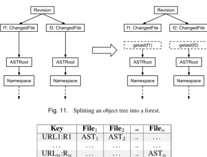
All of the data for a single project is processed inside of one Hadoop map task. This implies that the data for a project must fit in the memory of one map task (which on our cluster, is 1GB). Some projects are extremely large and can not fit their entire object tree in memory at one time (the largest project has over 6.5GB of data). To solve this problem, we split the object tree into a forest of disconnected trees.
Figure 11 shows a portion of an object tree on the left side. This is the sub-tree for one revision of a project, which contains two changed files. To split this tree, we simply turn theChangedFiles into leaves. This produces the forest on the right side of the figure.
When users wish to access the AST nodes for the changed filef1in the language, instead of read-ing an attribute of theChangedFileusers make a call togetast(f1). This call then retrieves and returns that changed file’s AST nodes. Once no references exist to any nodes in this sub-tree, they are free to be garbage collected. For most tasks, this solves the problem of fitting a project’s data into a map task’s process.
Since the AST trees are loaded on demand, we needed a storage strategy that allowed for random access reads. Our first choice was a distributed database named HBase [Apache Software Founda-tion 2014b], which is an open-source implementaFounda-tion of Google’s Bigtable [Chang et al. 2008]. We designed a table format for the AST objects:
ASTRoot f1: ChangedFile Revision Namespace ASTRoot f2: ChangedFile Namespace ASTRoot Revision Namespace ASTRoot Namespace f1: ChangedFile f2: ChangedFile getast(f1) getast(f2)
Fig. 11. Splitting an object tree into a forest.
Key File1 File2 .. Filen
URL1:R1 AST1 AST2 .. . . .
. . . .. . . .
URLn:Rn . . . .. ASTn
where each revision is a row in the table, indexed by a unique string containing the repository’s URL and the revision number. Each file in that revision is then stored in a column, using the file’s path as the column name. This was possible because the design of HBase allows creating columns on demand and empty cells take no space in the filesystem.
This design also allows for easily and incrementally updating the data. As our local cache is up-dated with new data from the remote repositories, we can simply insert rows for any new revisions. HBase provides Bloom filters [Bloom 1970] for more efficient random lookups, which we en-abled. Despite this optimization, our initial performance tests indicated that reads were much slower than we expected (described in detail in Section 5.3). Thus we designed a second storage strategy, this time using a flat-file datatype calledMapFile, provided by Hadoop.
A MapFile is actually two separate files. The first file is a list of key-value pairs called a SequenceFile. This file is sorted by the keys. In this new design, the previous HBase table is essentially linearized into a sortedSequenceFile:
Key Value Key Value .. Key Value
URL1:R1:F1 AST1 URL1:R1:F2 AST2 .. URLn:Rn:Fn ASTn
giving each cell a unique key by taking the HBase row key and concatenating the HBase column name.
The MapFiledata-structure also generates a second file, which is an index. For each block on the filesystem, it will store each block offset of the first file and the first key in each block. A random read becomes finding the block and scanning to find the key. As we show later, this new storage strategy performs substantially better.
Despite the performance benefit, using aMapFilecomes with a cost of the inability to perform incremental updates to the data. This is a restriction of the underlying distributed filesystem used by Hadoop, which states that files may only be appended. HBase circumvents this restriction by storing updates in memory and occasionally rewriting the underlying stores and merging in the new updates. With aMapFilewe would have to read and rewrite the entire file for a single, incremental update.
Our final storage strategy thus attempts to take the best of both worlds. First, all data is populated into HBase tables. This provides the easy incremental update of the data. From these tables we then generate aMapFile. Generating these files for use as input to mining tasks only takes a few hours and can be routinely scheduled.
4.5. Query Output Format
The output from a Boa program is a text file. The format of that file is described in this section. Consider the output variable declared in Figure 2:
rates : output mean[string] of int;
which declares an output variable named rates. This output variable collects intvalues and computes theirmean. The variable is indexed by astring, meaning that values are grouped by the index strings and for each unique index, a mean is computed.
For this example, the index is a project identifier. We expect to see in the output pairs of all project IDs and a single (mean) value. For example, the output from the program in Figure 2 is:
rates[100007] = 4.016949152542373 rates[100009] = 6.583333333333333 rates[100018] = 17.0 rates[100028] = 4.328990228013029 rates[100045] = 7.076923076923077 rates[100050] = 8.276806526806526 rates[100057] = 4.12 rates[100064] = 2.8446697996537225 rates[100081] = 1.0 rates[100083] = 5.2153846153846155 ...
In this output, each line represents a single project’s churn rate. The project’s unique identifier is the index (between the brackets) and the churn rate is on the right-hand side. Notice the variable’s name (rates) appears in the output. This is so if there is more than one output variable, you can distinguish them in the file.
Output lines are also sorted, lexicographically. Sorting is done from left to right by first sorting the output variable name and then by each index.
Finally, if an output variable takes a weight (such as top/bottom and minimum/maximum) then the weight value will show in the output. In this case, the output variable accepts values with weights, groups the output by the value, and then summarizes all the weights for each value. The output shows both the values and the (total) weights. For example, the output for the top-10 programming languages (task A1, Section 5.1) is:
counts[] = java, 50692 counts[] = c++, 40934 counts[] = php, 32696 counts[] = c, 30580 counts[] = python, 15352 counts[] = c#, 15305 counts[] = javascript, 12748 counts[] = perl, 9783 counts[] = unix shell, 4379 counts[] = delphi/kylix, 3842
In this case, the values are the programming languages and the weights are the number of projects using that language. The output only contains the top-10 highest weighted values.
5. EVALUATION
This section presents our empirical evaluation of the scalability and the usefulness of our language and infrastructure. The dataset used in this section contains all metadata about all SourceForge projects (700k+1) and repository metadata for only the Subversion or CVS repositories.
Programs were executed on a Hadoop [Apache Software Foundation 2014a] 1.2.1 install with 1 name node, 1 job tracker node, and 9 compute nodes. The compute nodes have a total of 116 CPU cores and 2GB memory per core. All machines run Ubuntu 12.04LTS. The cluster has been tuned for performance, including setting the maximum number of map tasks for each compute node equal 1This includes “user” projects, which aren’t listed.
to the number of cores on that node, increasing the VM heap size to 1GB per task, and enabling short-circuit local reads in the distributed filesystem.
5.1. Applicability
Our main claim is thatBoais applicable for researchers wishing to analyze ultra-large-scale software repositories. In this section we investigate this claim.
Research Question 1:Does Boa help researchers analyze ultra-large-scale software reposito-ries?
To answer this question, we examined a set of tasks (see Figure 12) that cover a range of different categories. For each task, we implemented aBoaprogram to solve the task. We also implemented pure Java and Hadoop [Apache Software Foundation 2014a] programs to solve the same tasks. The Java programs were written by an expert in mining software repositories and the Hadoop programs written by an expert in mining software repositories and Hadoop. They were then reviewed by a second person who is an expert in programming languages. The second person performed a code review and also simplified and condensed the programs to decrease the total lines of code as much as reasonably possible without impacting performance. This process substantially reduced (almost by half) the lines of code for the Java and Hadoop versions.
We were interested in investigating how Boa helps researchers along three directions: 1) are programs easier to write, 2) do those programs take (substantially) less time to collect the data, and 3) is the language expressive enough to solve such tasks. For each task, we collected two metrics: — Lines of code (LOC)2: the amount of code written
— Running time (RTime): the time to collect the data
All results are shown in Figure 12. The lines of code give an indication of how much effort was required to solve the tasks using each approach. For Java, the tasks required writing 32–180 lines of code and on average required 70 lines of code. Performing the same tasks inBoarequired at most 30 lines of code and on average less than 6 lines of code. Thus there were 6–22 times fewer lines of code when usingBoa.
Not shown in the table was the fact the Java programs also required using several libraries (for accessing SVN, parsing JSON data, etc). TheBoaprograms abstracted away the details of how to mine the data and thus the user was not required to use these additional, complex libraries.
The table also lists the time required to run each program and collect the desired data for the tasks. Note the Java programs accessed all JSON and SVN data from a local cache and the times do not include any network access. This was done for fairness, asBoaqueries also have a local cache of the JSON and SVN data. For the Java programs, there are three distinct groups of running times for programs that finished. The smallest times (A.1, A.2, B.1, B.2, and all of C and D) are tasks that only require parsing the project metadata and did not access any SVN data. The medium times (A.3, B.3, B.4, and B.5) accessed the SVN repositories but only required mining one (or very few) revisions. The largest times (B.6–B.11) all accessed the SVN repositories and mined most of the revisions to answer the task and thus required substantially more time. Finally note several tasks did not even finish within 24 hours (all of E). TheBoaprograms run in considerably less time. We see minimum speedups of 24 times but in the best case theBoaprogram solves the task over 569 times faster!
Research Question 2: Do Boa’s abstractions help researchers beyond general-purpose dis-tributed computing frameworks?
Comparing the Java andBoaversions shows a clear advantage toBoa, in terms of both lines of code and execution time. These Java versions are what most researchers would likely produce if trying to answer those questions. Some researchers might take the next step of trying to parallelize their analyses using a general-purpose distributed computing framework, such as Hadoop.
LOC R T ime (sec) T ask J a v a Boa Diff J a v a Boa Speedup A. Pr ogramming Languages 1. What are the ten most used programming languages? 61 3 20.33x 706 26 27.15x 2. Ho w man y projects use more than one programming language? 32 3 10.67x 691 25 27.64x 3. In which year w as Ja v a added to SVN projects the most? 89 9 9.89x 4,931 29 170.03x B. Pr oject Management 1. Ho w man y projects are created each year? 43 2 21.50x 725 25 29.00x 2. Ho w man y projects self-classify into each topic pro vided by SourceF or ge? 45 3 15.00x 658 27 24.37x 3. Ho w man y Ja v a projects using SVN were acti v e in 2011? 66 5 13.20x 4,627 24 192.79x 4. In which year w as SVN added to Ja v a projects the most? 107 5 21.40x 1,836 24 76.50x 5. Ho w man y re visions are there in all Ja v a projects using SVN? 60 4 15.00x 1,297 26 49.88x 6. Ho w man y re visions fix b ugs in all Ja v a projects using SVN? 76 5 15.20x 14,213 25 568.52x 7. Ho w man y committers are there for each Ja v a project using SVN? 69 5 13.80x 14,220 46 309.13x 8. Ho w man y Ja v a projects using SVN does each committer w ork on? 72 8 9.00x 13,789 27 510.70x 9. What are the churn rates for all Ja v a projects that use SVN? 68 4 17.00x 13,457 30 448.57x 10. Ho w did the no. of commits for Ja v a projects using SVN change o v er years? 79 5 15.80x 14,062 29 484.90x 11. F or all Ja v a projects using SVN, what is the distrib ution of commit log length? 82 5 16.40x 14,397 27 533.22x C. Legal 1. What are the fi v e most used licenses? 63 3 21.00x 673 26 25.88x 2. Ho w man y projects use more than one license? 32 3 10.67x 669 24 27.88x D . Platf orm/En vir onment 1. What are the fi v e most supported operating systems? 61 3 20.33x 639 26 24.58x 2. What are the projects that support multiple operating systems? 33 3 11.00x 723 26 27.81x 3. What are the fi v e most popular databases? 61 3 20.33x 609 25 24.36x 4. What are the projects that support multiple databases? 32 3 10.67x 678 26 26.08x 5. Ho w often is each database used in each programming language? 71 4 17.75x 655 27 24.26x E. Sour ce Code 1. Ho w man y fixing re visions added a null check? 180 30 6.00x 30,315 484 62.63x 2. What are the number of public methods (NPM), per project and per type? 137 13 10.54x >24h 753 >114.74x Fig. 12 . Se v eral exam ple mining tasks, with lines of code and ex ecution times (in seconds) for Ja v a and Boa programs solving the tasks.
LOC R T ime (sec) T ask Hadoop Boa Diff Hadoop Boa Speedup A. Pr ogramming Languages 1. What are the ten most used programming languages? 88 3 29.33x 24 26 0.92x 2. Ho w man y projects use more than one programming language? 43 3 14.33x 26 25 1.04x 3. In which year w as Ja v a added to SVN projects the most? 59 9 6.56x 27 29 0.93x B. Pr oject Management 1. Ho w man y projects are created each year? 46 2 23.00x 25 25 1.00x 2. Ho w man y projects self-classify into each topic pro vided by SourceF or ge? 44 3 14.67x 25 27 0.93x 3. Ho w man y Ja v a projects using SVN were acti v e in 2011? 61 5 12.20x 25 24 1.04x 4. In which year w as SVN added to Ja v a projects the most? 71 5 14.20x 22 24 0.92x 5. Ho w man y re visions are there in all Ja v a projects using SVN? 53 4 13.25x 24 26 0.92x 6. Ho w man y re visions fix b ugs in all Ja v a projects using SVN? 69 5 13.80x 24 25 0.96x 7. Ho w man y committers are there for each Ja v a project using SVN? 49 5 9.80x 30 46 0.65x 8. Ho w man y Ja v a projects using SVN does each committer w ork on? 48 8 6.00x 24 27 0.89x 9. What are the churn rates for all Ja v a projects that use SVN? 60 4 15.00x 26 30 0.87x 10. Ho w did the no. of commits for Ja v a projects using SVN change o v er years? 46 5 9.20x 25 29 0.86x 11. F or all Ja v a projects using SVN, what is the distrib ution of commit log length? 46 5 9.20x 25 27 0.93x C. Legal 1. What are the fi v e most used licenses? 88 3 29.33x 24 26 0.92x 2. Ho w man y projects use more than one license? 43 3 14.33x 24 24 1.00x D . Platf orm/En vir onment 1. What are the fi v e most supported operating systems? 88 3 29.33x 25 26 0.96x 2. What are the projects that support multiple operating systems? 35 3 11.67x 24 26 0.92x 3. What are the fi v e most popular databases? 88 3 29.33x 24 25 0.96x 4. What are the projects that support multiple databases? 35 3 11.67x 25 26 0.96x 5. Ho w often is each database used in each programming language? 46 4 11.50x 26 27 0.96x E. Sour ce Code 1. Ho w man y fixing re visions added a null check? 226 30 7.53x 496 484 1.02x 2. What are the number of public methods (NPM), per project and per type? 220 13 16.92x 749 753 0.99x Fig. 13 . The same example mining tasks, with lines of code and ex ecution times (in seconds) for Hadoop and Boa programs solving the tasks.
To answer this question, we created optimized Hadoop versions of each task. This step re-uses the exact same input data thatBoauses. As such, unlike the Java versions that required many libraries for processing JSON, SVN, etc, the Hadoop versions benefited from the pre-processing we did for Boa.
The results, shown in Figure 13, show that the performance of the hand optimized Hadoop ver-sions is about on par with that ofBoa, withBoabeing on average 2% slower then the hand optimized Hadoop versions. The Hadoop versions have on average 13 times more lines of code more compared to theBoaversions. This shows that users can easily produce fast, parallel code usingBoa, but with many fewer lines of code and without having to learn how to write Hadoop programs.
5.1.1. Detailed Examples. Figures 14–17 show four interestingBoaprograms used to solve some of the tasks. These programs highlight several useful features of the language.
1counts: output sum[int] ofint; 2p: Project = input;
4HasJavaFile := function(rev: Revision): bool { 5 exists (i: int; match(‘.java$‘, rev.files[i].name)) 6 return true;
7 return false; 8}
10 foreach (i: int; def(p.code_repositories[i]))
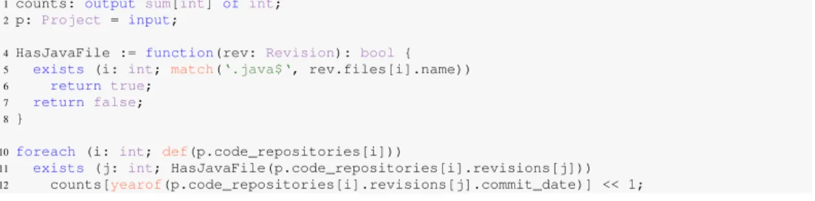
11 exists (j: int; HasJavaFile(p.code_repositories[i].revisions[j])) 12 counts[yearof(p.code_repositories[i].revisions[j].commit_date)] << 1;
Fig. 14. Task A.3: Querying years when Java files were first added the most.
Figure 14 answers task A.3 and demonstrates the use of a user-defined functions. The function HasJavaFile(line 4) takes a singleRevisionas argument and determines if it contains any files with the extension “.java”. If the revision contains at least one such file it returnstrue. This function is used in thewhenstatement (line 11) as the boolean condition.
1counts: output sum of int; 2p: Project = input;
4exists (i: int; match(‘^java$‘, lowercase(p.programming_languages[i]))) 5 foreach (j: int; p.code_repositories[j].url.kind == RepositoryKind.SVN) 6 foreach (k: int;isfixingrevision(p.code_repositories[j].revisions[k].log)) 7 counts << 1;
Fig. 15. Task B.6: Querying number of bug-fixing revisions in Java projects using SVN.
Figure 15 answers task B.6 and makes use of the built-in functionisfixingrevision(line 6). The function uses a list of regular expressions to match against the revision’s log. If there is a match, then the function returns true indicating the log most likely was for a revision fixing a bug.
1counts: output top(5) of string weight int; 2p: Project = input;
4foreach (i: int; def(p.licenses[i])) 5 counts << p.licenses[i] weight 1;
Figure 16 answers task C.1 and makes use of atop aggregator(line 1). The emit statement (line 5) now takes additional arguments giving a weight for the value being emitted. The top aggregator then selects the top N results that have the highest total weight and gives those as output.
1counts: output sum[string][string] of int; 2p: Project = input;
4foreach (i: int; def(p.programming_languages[i])) 5 foreach (j: int; def(p.databases[j]))
6 counts[p.programming_languages[i]][p.databases[j]] << 1;
Fig. 17. Task D.5: Querying pairs of how often each database is used in each programming language.
Figure 17 answers task D.5 and makes use of a multi-dimensional aggregator (line 1) to output pairs of results. Again, theemitstatement (line 6) is modified. This time, the statement requires providing multiple indexes for the table.
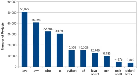
5.1.2. Results Analysis. We also show some interesting and potentially useful results from four of the tasks. For example, Figure 18 shows the results of Task A.1 and charts the ten most used programming languages on SourceForge. 9 of the 10 languages appear in the top-12 of the TIOBE Index [BV 2012]. Languages such as Visual Basic did not appear in our results despite being #6 on the TIOBE index. This demonstrates that while the language is popular in general, it is not popular in open source. Similarly Objective-C did not appear in our results, as most programs written in Objective-C are for iOS and are (most likely) commercial, closed-source programs, or not typically hosted on SourceForge.
java c++ php c python c#
java-script perl unix shell delphi/kylix
0 10,000 20,000 30,000 40,000 50,000 60,000 50,692 40,934 32,696 30,580 15,352 15,305 12,748 9,783 4,379 3,842 N u m b er o f P ro je ct s
Fig. 18. Task A.1: Popularity of programming languages on SourceForge.
The results of Task B.7 are shown in Figure 19. Note that the y-axis is in logarithmic scale. These results show that a large number of open-source projects have only a single committer. Generally, open-source projects are small and have very few committers and thus problems affecting large development teams may not show when analyzing open-source software.
Task B.8 looks at this data from the other angle. Figure 20 shows the number of projects each unique committer works on. Again, the vast majority of open-source developers only work on a single project. Only about 1% of committers work on more than three projects!
1 2 3 4 5 6 7 8 9 10 11 12 13 14 15 16 17 18 19 20+ 1 10 100 1,000 10,0009,189 2,190 1,020 625 333 244 153 141 90 66 42 47 38 33 21 31 28 15 20 213 Number of Committers N u m b er o f P ro je ct s
Fig. 19. Task B.7: number of committers in each Java project using SVN. NOTE: y-axis is in logarithmic scale.
1 2 3 4 5 6 7 8 9 10 11 12 13 14 15 1 10 100 1,000 10,000 100,000 25,690 2,625 587 194 78 37 20 3 5 3 3 1 Number of Projects N u m b er o f C o m m it te rs
Fig. 20. Task B.8: number of Java projects each SVN committer works on. NOTE: y-axis is in logarithmic scale.
Another interesting result came from Task B.11 and is shown in Figure 21. This task examines how many words appear in log messages. First, around 14% of all log messages were completely empty. We do not investigate the reason for this phenomenon but simply point out how prevalent it is. Second, over two thirds of the messages contained 1–15 words, which is less than the average length of a sentence in English. A normal length sentence in English is 15–20 words (according to various results in Google) and thus we see that very few logs (10%) contained descriptive messages. 5.2. Scalability
One of our claims is that our approach is scalable. We investigate this claim in terms of scaling the size of the cluster and scaling the size of the input.
Research Question 3:Does our approach scale to the size of the cluster?
To answer this question, we run one sample program from each category listed in Figure 12 using our SourceForge.net dataset. We fix the size of the input to 700k projects and vary the number
15% 73% 7% 4% 1% 0 1-15 16-25 26-50 51 or more
Fig. 21. Task B.11: number of words in SVN commit logs for Java projects.
of available map slots in the system from 1–116 (note: our current cluster only has 116 cores). Figure 22 shows the results of this analysis where each group represents one of the sample programs, the y-axis (in logarithmic scale) is the total time taken in seconds to run the program, and the x-axis is the number of available map slots in the cluster. Each value is the average of 10 executions.
Task A.3 Task B.6 Task C.1 Task D.5 Task E.1
1 10 100 1,000 10,000
1 map 2 maps 4 maps 8 maps 16 maps 32 maps 64 maps 128 maps
E x e c u t i o n t i m e ( s e c o n d s )
Fig. 22. Scalability of sample programs. Y-axis is total time taken. X-axis is the number of available map slots in the cluster. NOTE: y-axis is in logarithmic scale.
As one might expect, the Hadoop framework works well with this large dataset. As the maximum number of map slots increases, we see substantial decreases in execution time as more parallel map slots are being utilized.
Note that with our current input size of 700k projects, the maximum number of map slots needed for programs not analyzing source code is 34. Thus we don’t generally see any benefit when in-creasing the maximum map slots past that. As we increase the size of our input however, we would expect to see differences in these data points indicating scaling past 34 map slots. We do see scaling past that for the last program, which analyzes source code.
Research Question 4:Does our approach scale with the size of the input?
To answer this question, we fix the number of compute nodes to 6 (with a total of 44 map slots available) and then vary the size of the input (7k, 70k, and 700k projects). The results for all tasks in Figure 12 are shown in Figure 23. We compare against the programs written in Java to answer the