On the Conditional Effects of IMF Program Participation on Output Growth

On the Conditional Effects of IMF Program

Participation on Output Growth

Michael Binder

Marcel Bluhm

CES

IFO

W

ORKING

P

APER

N

O

.

3161

C

7:

M

P

I

F

A

2010

An electronic version of the paper may be downloaded

• from the SSRN website: www.SSRN.com

• from the RePEc website: www.RePEc.org

CESifo Working Paper No. 3161

On the Conditional Effects of IMF Program

Participation on Output Growth

Abstract

The empirical evidence currently available in the literature regarding the effects of a country's

IMF program participation on its output growth is rather mixed. To shed new evidence on this

issue, in this paper we specify a state-dependent panel data model accounting in particular for

program participation selection and the potential conditionality of the output growth effects of

program participation on a country's degree of program implementation and institutional

factors such as quality of governance, internal stability, health, and educational attainment.

We find that the effects of IMF program participation on output growth vary systematically

with the degree of program implementation as well as our index of institutional factors, and

that these effects are positive only if the IMF program is implemented to a sufficient degree or

if the program participation is coupled with sufficient progress in improving institutional

quality.

JEL-Code: O11, O19, C33.

Keywords: IMF program participation, output growth, panel sample selection models,

conditional pooling.

Michael Binder

Goethe University Frankfurt

House of Finance

Grueneburgplatz 1

Germany - 60323 Frankfurt am Main

[email protected]

Marcel Bluhm

Goethe University Frankfurt

House of Finance

Grueneburgplatz 1

Germany - 60323 Frankfurt am Main

[email protected]

We are grateful for comments and suggestions from two conference discussants, Michel

Beine and Jörg Breitung, as well as seminar and conference participants at Bonn University,

1

Introduction

The International Monetary Fund (IMF) began its operations in 1945, and was conceived as an independent international organization helping to pro-mote macroeconomic and financial stability as well as growth of the world economy. In the 1970s the IMF expanded its role towards providing on a conditional basis development assistance to countries that as a prerequisite for loan approval had to initiate economic and structural reforms as

out-lined by the IMF.1 While the IMF has often been criticized for failures in

carrying out such development policy, in the wake of the recent financial crisis a number of calls have been made for an expanded role of the IMF. This paper re-considers the effects of a country’s participation in IMF loan programs on its output growth, taking account of conditionality of these growth effects on the degree of program implementation as well as institu-tional factors such as quality of governance, internal stability, health, and educational attainment.

The IMF has been offering four types of loan arrangements involving policy conditions, the stand-by arrangement (SBA), the extended fund fa-cility (EFF), the structural adjustment fafa-cility (SAF), and the enhanced structural adjustment facility (ESAF), subsequently replaced by the poverty reduction and growth facility (PRGF). Most of the IMF’s assistance is pro-vided through SBAs. Designed in 1952 to help countries with addressing short-term balance of payments problems, SBAs typically cover periods of one to two years. The EFF was set up in 1974 to help countries encoun-tering long-term balance of payments problems requiring fundamental eco-nomic reforms. EFF loan arrangements usually cover three to five years. The SAF has been used since 1986, and is designed to provide assistance for low-income countries. The ESAF only differs slightly from the SAF, but involves stricter conditionality criteria and larger loan amounts. The ESAF was used since 1986; after the East-Asian crisis this facility was relabeled PRGF, as it was broadened to include poverty reduction and to grant gov-ernments larger scope in negotiating the policy conditions. Typically PRGF programs are pursued for up to four years. When conditionality is involved, the IMF assesses whether a country complies with the conditionality re-quirements; if so, the country can draw on the loan funds in pre-specified

1

intervals.2

The previous empirical evidence regarding the effects of a country’s par-ticipation in IMF loan programs on its output growth is rather mixed. Us-ing political economy variables as instruments to address endogeneity issues, Barro and Lee (2005) find that the IMF loan program participation rate has

a negative effect on output growth.3 Vreeland (2003), using counterfactual

analysis, also finds evidence that program participation leads to a reduction of output growth. In contrast, Dicks-Mireaux, Mecagni and Schadler (2000), also using counterfactual analysis, find positive output growth effects of IMF program participation.

In this paper we provide new insights regarding the effects of a coun-try’s IMF program participation on its output growth by constructing and estimating a state-dependent panel data model accounting in particular for sample selection, for the endogeneity of program participation, and for the potential conditionality of the output growth effects of IMF program partic-ipation on a country’s degree of program implementation and institutional factors such as quality of governance, internal stability, health, and edu-cational attainment. We argue that capturing sample selection, program participation endogeneity, and state dependence of the effects is critical for properly measuring the effects of a country’s IMF program participation on output growth. To cope with sample selection issues, we work with an equation system composed both of a program participation selection and an output growth (participation effects) equation; within this equation system, we account for the endogeneity of the program participation measure in the output growth equation using a two-step maximum likelihood estimator. We capture country-specific effects under the two alternatives of a random and a fixed effects model. To account for the state dependence of the output growth effects of IMF program participation, we use semi-parametric con-ditional pooling techniques to condition the effects of participation in IMF programs on a country’s degree of program implementation and its

institu-2

For the empirical work in this paper we will not discriminate between these different loan arrangement schemes. While SBAs in contrast to the other schemes cover elements of structural reforms only to a limited extent, for example in the form of exchange rate and pricing policies, SBAs often precede one of the other schemes simply because “there has not [...] been enough time to assemble all the necessary elements of a comprehensive structural package” (Polak, 1991).

3_{Barro and Lee (2005) define the loan participation rate as the fraction of months} during a five-years interval that a country operated under IMF loan programs.

tional features as measured by our index comprising measures of quality of governance, internal stability, health, and educational attainment.

Using this novel econometric framework and a sample of annual data for 86 countries over the time period from 1975 to 2005, we provide evi-dence that the effects of IMF program participation on output growth vary systematically with the degree of program implementation as well as our index of institutional factors, and that these effects are positive only if IMF program participation is at a sufficiently advanced stage, or if the program participation is coupled with sufficient progress in improving institutional quality.

The remainder of this paper is structured as follows: Section 2 pro-vides a review of the previous literature. Sections 3 and 4 describe our panel econometric framework, with Section 3 focussing on sample selection and endogeneity issues, and Section 4 describing our approach to modelling state dependence of the effects of IMF program participation. Section 5 de-scribes the construction of our variables for modelling the state dependence of the effects of IMF program participation on a country’s output growth. Section 6 presents our empirical results. Finally, Section 7 concludes. Fur-ther details regarding our econometric modelling framework and inference approach, further results checking on the robustness of our main findings and some details concerning the data set we collected for this paper are described in several appendices.

2

Review of Previous Literature

There are a number of notable contributions to the literature concerned with measuring the effects of a country’s IMF loan program participation on output growth. Most of the contributions can be characterized as following one of three approaches: (i) the “before-after”-approach, (ii) the

“with-without”-approach, and (iii) regression-based approaches.4

The “before-after”-approach is based on the idea that, ceteris paribus,

output growth that a country has experienced before/after entering an IMF loan program may be compared with output growth that the country experi-ences during participation in an IMF loan program. For example, Evrensel

4

See also Vreeland (2003) and Dreher (2006) for a similar categorization of the litera-ture.

(2002) investigates the effects of IMF loan programs for a sample of 109 countries over the time period from 1971 to 1997 using lags of up to three years before and after program participation to conduct a “before-after” analysis. With respect to the output growth effects of program participa-tion, she argues that the evidence is inconclusive. The main problem with the “before-after” approach, in any case, is that in practice it does not allow to fully account for country-specific factors that have bearing on the output growth effects of program participation.

The “with-without” approach rests on the assumption that the core fea-tures of countries that participate in IMF loan programs are the same as those of countries not participating in IMF loan programs. For example, us-ing matchus-ing methods, Hutchison (2004) analyzes the differences in output growth between countries participating and those not participating in IMF loan programs, for a panel of 25 countries over the time period 1975 to 1997. Hutchison’s (2004) results suggest that, once sample selection is controlled

for using observed variables only,5 participation in IMF loan programs has

no adverse effects on output growth. However, Hutchison’s (2004) match-ing methods do not take into account any selection based on unobserved variables, and so his results may still be subject to sample selection bias. Bordo and Schwartz (2000) compare the performance of 24 Asian and Latin-American countries over the time period 1973 to 1999 and find that before the onset of currency or banking crises, output growth declines more strongly in countries not participating in IMF loan programs, though not to levels as low as of those countries participating in IMF loan programs. They find furthermore that countries not participating in IMF loan programs recover faster after currency and banking crises.

The majority of contributions to the empirical literature on the effects of IMF loan program participation on output growth employ regression-based approaches. Dicks-Mireaux, Mecagni, and Schadler (2000) perform a counterfactual analysis using a panel data set for 74 countries over the time period from 1986 to 1991. Taking into account sample selection issues, they find significant, positive effects of IMF loan program participation on output growth. In contrast, Vreeland (2003) using a similar methodology for a panel

5

See, for example, Heckman, Ichimura, and Todd (1998) for a distinction between selection based on observed variables versus selection based on unobserved variables.

of 79 countries over the time period from 1970 to 1990,6 finds a negative im-pact of IMF program participation on output growth. Bordo and Schwartz (2000), also using counterfactual analysis, find negative but insignificant ef-fects on output growth during the onset of a currency or banking crisis, but positive and significant effects a year later. Their data set comprises 24 Asian and Latin-American countries and covers the time period from 1973 to 1998. Hutchison and Noy (2003), distinguishing between IMF program approval and successful completion of IMF programs, analyze the effects of IMF program participation on output growth in a sample of 65 develop-ing countries over the time period from 1975 to 1997. Usdevelop-ing counterfactual analysis, they find that participation in IMF loan programs results in short-run output growth losses, though noting that these results appear entirely driven by the Latin-American countries in their sample. Finally, Barro and Lee (2005), using a set of political economy variables as instruments to cor-rect for regressor endogeneity problems in a panel comprising 86 countries over the time period from 1975 to 2000 find that participation in IMF loan programs has a significantly negative effect on output growth.

3

Panel Data Models with Sample Selection and

Censored Endogenous Variables

When using a regression framework to estimate the effects of IMF pro-gram participation on a country’s output growth, two issues that need to be addressed are (i) endogeneity of the program participation measure in the output growth equation and (ii) sample selection. The first issue arises when

explaining output growth with,inter alia, a country’s participation in IMF

loan programs, as one will need to distinguish whether a country’s economic performance is causal for IMF program participation, or vice versa. The second issue arises when using non-randomly selected samples for model es-timation, as then the fact that the output growth performance of countries that participate in IMF programs may systematically differ from that of

those countries that do not participate needs to be addressed.7 Countries

tend to participate in IMF loan programs when they encounter economic

6_{Vreeland (2003) also uses a larger data set, ranging from 1950 to 1990.} 7

As is well known, the investigation of such sample selection effects was pioneered in empirical microeconomics by Heckman (1979).

problems, which implies that they are likely to experience an output growth process that is different from that of countries that do not turn to the IMF for assistance. It is thus sensible to analyze the output growth process of participating countries – that are likely to be in a situation of economic crisis – separately from the output growth process of non-participating countries, which in turn necessitates to correct for sample selection. As noted by Vella (1998), while sample selection has in the literature been commonly con-fronted in purely cross-sectional analyses, it is less frequently considered to be of concern in the estimation of panel models. This may in part be due to the perception that a panel model incorporating random or fixed effects will eliminate most forms of unobserved heterogeneity. However, consistency of the fixed effects estimator of a default fixed effects model not explic-itly capturing the selection mechanism requires that the selection operates purely through the time-invariant country-specific terms, which appears to be rather unlikely. Consistency of the random effects estimator of the de-fault random effects panel model requires the additional condition that the time-invariant country-specific effect and the model’s disturbance term are uncorrelated.

3.1 Random Effects Panel Model with Sample Selection and

Endogeneity

In the following we will first outline a random effects model to correct for sample selection as well as endogeneity of the IMF program participation measure in the output growth equation. Our exposition of this random

ef-fects model draws strongly upon Vella (1998) and Vella and Verbeek (1999).8

Consider the following random effects panel data model with sample selec-tion and endogeneity:

8_{Vella and Verbeek (1999) discuss a model thatinter alia allows for a broader range} of functional forms than we wish to consider in this paper. Our model specification also differs from theirs in that unlike Vella and Verbeek (1999) we wish to allow for a larger number of regressors in the participation selection equation than in the participation effects equation.

y_it∗ =µi+ditθ+xxx0itβββ+eit (1)

(“participation effects equation”),

d∗_it=αi+zzz0itγγγ+vit (2)

(“participation selection equation”),

d∗_it= ( d∗_it ifd∗_it>0, 0 otherwise, (3) yit= ( y_it∗ ifdit>0, “unspecified” otherwise, (4)

i = 1,2, ..., N, and t = 1,2, ..., Ti, where y∗_it and d∗_it are latent endogenous

variables for country i and time period t with observed counterparts yit

(output growth – participation effects measure) and dit (IMF loan-quota

ratio – measure of participation intensity).9 Also note thatxxxit is a subset ofzzzit, and throughout our exposition in this sectionzzzit will be taken to be strictly exogenous.

Let us write the unobserved component of each equation as the sum of

the country-specific random effect (µi in Equation (1) and αi in Equation

(2)) and the time-specific idiosyncratic error term (eit in Equation (1) and

vit in Equation (2)):

it=µi+eit, (5)

and

uit =αi+υit. (6)

Defining uuui as the stacked (Ti ×1) vector of uit’s for country i, XXXi =

9_{While the availability of data on output growth is per se not tied to a country} partici-pating in an IMF loan program (that is,dit≥0),yitunder non-participation is unobserved

from the perspective of the sample selection model equations in (1) and (2), in that it is then driven by a different model of output growth.

(xxxi1, xxxi2, ..., xxxiTi) 0_{, andZZZ} i = (zzzi1, zzzi2, ..., zzziTi) 0_{, we assume that} u u ui|ZZZiiid∼ N(0, σα2ιιιιιι0+σv2III), (7) withιιιbeing a Ti×1 vector of ones. Equation (7) restrictsαi and vit to be

independent acrossi, andvitis restricted to be intertemporally uncorrelated

and homoskedastic. We also assume that

E(it|ZZZi, uuui) =τ1uit+τ2u¯i, (8) where ¯ui =T_i−1PT_t=1i uit, andτ1andτ2 are parameters. Note that Equation

(8) allows for dit and it to be correlated, capturing endogeneity of the

IMF loan-quota ratio in the output growth equation as arising through the program participation selection mechanism specified in Equation (2). Also,

throughτ2 6= 0 Equation (8) allowseit to be intertemporally correlated and

heteroskedastic.

Conditioning Equation (1) on the selection outcomes,dddi, as well as the

regressors inXXXi, and observing Equation (8) yields

E(y∗_it|ZZZi, dddi) = ditθ+xxx0itβββ+E(it|ZZZi, dddi)

= ditθ+xxx0itβββ+τ1uit+τ2u¯i. (9)

To obtain the sample selection correction terms in uit and ¯ui on the

right-hand side of Equation (9), Vella and Verbeek propose to compute

E[uit|ZZZi, dddi] =

Z

[αi+E(vit|ZZZi, dddi, αi)]f(αi|ZZZi, dddi)dαi, (10)

where f(αi|ZZZi, dddi) denotes the conditional density of αi, and vit in terms of its expectation conditional on ZZZi, dddi, and αi is the generalized residual

from estimation of the panel Tobit model in Equation (2).10 _{The conditional}

density ofαi can be obtained from

f(αi|ZZZi, dddi) =

f(dddi|ZZZi, αi)f(αi)

f(dddi|ZZZi)

, (11)

10

See Gourieroux, Monfort, Renault, and Trognon (1987) for a definition of the gener-alized residuals we work with here.

withf generically denoting density functions, and where f(dddi|ZZZi) = Z Ti Y t=1 f(dit|ZZZi, αi)f(αi)dαi. (12)

After obtaining the conditional expectation of uit in Equation (10), the

output growth equation in (1) can be estimated, including uit and ¯ui as

additional variables to correct for sample selection while also allowing for

endogeneity of dit. The functional form of Equation (10) as well as

de-tails concerning the computation of the standard errors for the estimates of

θ, βββ, τ1, and τ2 can be found in Appendix A.

Ifeitis to be restricted to be intertemporally uncorrelated, then Equation

(8) reduces to

E(it|ZZZi, uuui) =τ1uit, (13) implying that Equation (10) simplifies to

E[uit|ZZZi, dit] =

Z

[αi+E(vit|ZZZi, dit, αi)]f(αi|ZZZi, dit)dαi. (14)

3.2 Fixed Effects Panel Model with Sample Selection and

Endogeneity

Semykina and Wooldridge (2005) propose a fixed effects specification of a panel data model closely related to Equations (1) to (4). In what follows we will invoke Semykina and Wooldridge’s (2005) modelling of the fixed effects, decomposing the fixed effects into a systematic component driven by

observables (the variables ingggi) as well as a random unobserved component,

and then embed the resultant model within the estimation and inference

procedure discussed in Sub-Section 3.1.11

Following Semykina and Wooldridge (2005), let us thus invoke a Mundlak (1978) type decomposition of the country-specific fixed effect in Equation

11_{Semykina and Wooldridge (2005) provide a different two-step estimation and inference} procedure for a panel model with a Probit specification of the selection mechanism than we propose in this sub-section for a panel model with a Tobit specification of the selection mechanism. For our data set, the procedure we outline here appears to be more robust to the selection of variables ingggi than the Semykina and Wooldridge (2005) procedure.

A systematic comparison of our procedure with that of Semykina and Wooldridge (2005) would be interesting to pursue but is beyond the scope of this paper.

(2):

αi = ζ+gggi0κκκ+ri, (15)

whereri is a random effect; defining

˜

uit =ri+vit, (16)

we assume in analogy to Equation (7) that ˜

u

uui|ZZZi, ζ, gggi iid

∼ N(0, σ_r2ιιιιιι0+σ2_vIII). (17)

Note that the systematic component in αi, gggi, consists of cross-sectional

means over time, that is country-specific constants.

Clearly, the Mundlak (1978) and Semykina and Wooldridge (2005) fixed effects specification restricts the systematic variation of the country-specific

effect to only arise through the vector of observables gggi. This is a more

restrictive specification of the fixed effect than often adopted in other panel

data models, for example in the linear dynamic panel data literature.12

Let us use a similar decomposition as specified in Equation (15) for the country-specific effect in the participation selection equation also for the country-specific effect in the output growth (participation effects) equation (that is, Equation (1)):

µi = ψ+qqq0iφφφ+χi, (18)

whereχi is a random effect andqqqi is a subset of gggi; defining ˜

it=χi+eit, (19)

we now also assume in analogy to Equation (8) that

E(˜it|ZZZi,uuu˜i, ψ, qqqi) = ˜τ1u˜it+ ˜τ2u¯˜i. (20) Note thatggg is a subset ofqqq.

Under Equations (15) to (20), we therefore allow for a less restrictive

12_{See, for example, Binder, Hsiao, and Pesaran (2005) for an unrestricted formulation} of fixed effects within a linear dynamic panel data model.

specification of the country-specific effects than in Vella and Verbeek (1999), and capture a fixed effects specification in the spirit of Mundlak (1978) and Semykina and Wooldridge (2005), augmenting both the program selection equation, Equation (2), and the output growth equation, Equation (1), with the regressors inqqqi andgggi, but otherwise pursuing the estimation and infer-ence procedure of Sub-Section 3.1. We will discuss the choice of elements in

qqqi in Section 6.

Finally, the null of the random effects specification of Sub-Section 3.1 can be tested against the fixed effects specification of this section by investigating whetherκκκ= 000 andφφφ= 000.

4

Conditioning the Effect of IMF Loan Program

Participation

The fixed effects model of Section 3 still involves the restriction that the systematic differences in the output growth processes across participating countries can be captured through the country-specific effects and different realizations of the regressors indit andxxxit. This is a rather strong assump-tion. To analyze the effects of IMF program participation, it clearly seems desirable to allow for systematic differences in these effects themselves across countries. To do so in a parsimonious form that also allows us to learn about the sources of the variations of the effects across countries, we consider here the conditional pooling (state dependence) approach of Binder and Offer-manns (2008). This approach allows us to model the conditionality of the growth effects of IMF loan programs on a country’s degree of program imple-mentation or on its institutional quality with a minimal set of assumptions regarding the functional form of this conditionality. The approach consists of modelling the state dependence with flexible functional form polynomials, as a (cross-sectionally) homogeneous function of the relevant conditioning

variable. Denoting the conditioning variable by wit and the flexible

func-tional form polynomial byθ(wit), Binder and Offermanns (2008) propose to

specifyθ(wit) using a parametric function of flexible form, and in particular choose Chebyshev polynomials as one specification of orthogonal

polynomi-als: θ(wit) = τ X s=0 γ_s(θ)cs(wit), (21)

with the Chebyshev polynomials cs(wit) recursively defined as cs+1(wit) =

2witcs(wit)−cs−1(wit), s= 1,2, ..., τ, c0(wit) = 1, c1(wit) =wit, and where

γs(θ),s= 0,1, ..., τ, are coefficients that are homogeneous across countries.13 To condition an independent variable’s effect, the variable may be

mul-tiplied with the Chebyshev polynomial θ(wit), and estimation can then be

carried out as usual with the resultant augmented set of variables.

5

Conditioning Variables

Under the conditional pooling approach (some of) the model coefficients are a function of a conditioning variable. According to the IMF, “[c]onditionality refers to policies and actions that a borrowing member agrees to carry out as a condition for the use of IMF resources. The purpose of conditionality is to ensure assistance to members [...] in a manner that [...] establishes adequate

safeguards for the temporary use of the IMF’s resources.”14 _{In practice, the}

IMF only disburses installments of funds agreed to in the loan program if the country initiates specific reforms, that is, complies with conditionality of the loan program. Hence, one way to model compliance with conditionality is to consider the ratio of loans actually drawn relative to loans originally

agreed upon.15 Provided that the IMF consistently disburses funds only

to countries that are sufficiently successful in advancing economic reforms, the loans-drawn-to-agreed ratio should be a useful proxy as to whether a country is successful in implementing the economic reforms advocated by the IMF.

We also consider a more direct measure of structural conditionality. Structural conditionality according to the IMF since the 1980s has involved

changes in policy processes, legislation, and institutional reforms.16 In line

13

Chebyshev polynomials belong to the class of orthogonal polynomials, and thus can address collinearity problems that could arise underτ >1.

14

See Fritz-Krockow and Ramlogan (2007), p. 25.

15_{This measure was initially suggested as a proxy for compliance with conditionality by} Killick (1995)

16

with this, the IMF is arguing that “the implementation of IMF-supported programs depends to a significant extent on the domestic political and

insti-tutional environment”.17 By fostering institutional development, the IMF

in effect acknowledges that efficient outcomes in market-oriented economies are most likely to occur when the non-market institutions are functioning well. Rodrik (2009) distinguishes between five types of institutions that al-low markets to perform well: (i) private property rights give enterpreneurs the security of claiming the gains from investment and innovations; (ii) reg-ulatory institutions prevent market failures that can arise from fraudulent behavior and incomplete information; (iii) institutions for macroeconomic stabilization are neccessary to alleviate shocks that hit the economy; (iv) institutions for social security render a market economy compatible with social coherence and stability; and (v) institutions of conflict management are neccessary to prevent social conflicts from creating uncertainty and di-version of ressources from economically productive activities. To capture a broad range of aspects of institutional quality, we construct for this paper an index incorporating measures of bureaucracy quality, absence of corruption, law and order, government stability, absence of ethnic tensions and internal conflicts, and add two further dimensions by also taking account of health (life expectancy) and educational attainment. The set up of the index is

described in what follows.18 The index is constructed on the basis of the

mean of thej-th country’s index elements relative to the mean of the same

index elements for a base-country year (the United States in 2000):

indexit=

Pm

s=1 s-th variableit

Pm

s=1 s-th variablebase-country, base-year

, (22)

wherem denotes the number of variables that enter into the construction of

the index. To be able to calculate this index, we replace missing observations

using interpolated values. If for, say, country i a time series is missing

entirely, we proxy it via a “rank-matching” procedure: For each time period

for countryi, first a preliminary index is calculated on the basis of Equation

(22) involving only those variables that are actually available for country i.

We then also calculate the same preliminary index for all other countries

17

See International Monetary Fund (2006). 18

A listing including a description of all variables used for construction of our index is given in Appendix B.

for time period t, excluding those variables that are completely missing for

country i. Using these preliminary indices, we then calculate the period

t relative rank (that is, rankit

number of countriest) of the preliminary index value

of country i among the set of all countries that can be considered for the

preliminary index values in period t. We then proxy for time period t the

variable in countryi that is entirely missing with the value of that variable

for which the periodtrelative rank is closest to the relative rank calculated

for countryi’s preliminary index for period t.

Finally, we impute those variables for which there are no observations either at the beginning or at the end of the series backward or forward, respectively, using the percentage changes of, again, a preliminary index that contains only the variables that are available for the country in the missing time period. At this point we then have for each country a balanced set of variables that can be used to calculate the index as outlined in Equation (22).

Our approach to index calculation ensures that there are no mean-shifts in the index if for a country the time series for some variable begins later or ends earlier than the time series for some other variables for that country. Our approach furthermore preserves all the information about the variation in the time series we exploit. It should be noted that due to the imputation procedure it is possible that an index value may become larger than one.

6

Empirical Results

We begin by discussing empirical results obtained when taking into account sample selection and regressor endogeneity by means of considering the fixed effects panel model without state dependence of effects, as outlined in

Sub-Section 3.1.19 _{The selection equation, Equation (2) is a fixed effects Tobit}

19

The set of regressors for all equations was chosen on the basis of the Akaike Information Criterion (AIC). Since the AIC turned out to always select the fixed effects specification, in what follows we focus our discussion on the fixed effects model. Potential candidates for the Mundlak variables,giandqi, were a country’s fertility rate, freedom of the press,

freedom status of society, economic proximity to the U.S. and economic proximity to major Europe. Results for the random effects specification are provided as robustness check in Appendix D. Potential candidates forzzzit and xxxit were a country’s cumulative

number of years in IMF loan programs, quota share at the IMF, staff share at the IMF, political proximity to the U.S., political proximity to major Europe, reserve position, current account position, trade openness, democracy index rating, investment share of GDP, Government share of GDP, and inflation.

model, as the loan-quota ratio is left-censored at zero. It contains country years with and without participation in IMF loan programs. Note that when later we turn to considering state dependence of effects, the estimated models involve different sets of observations than considered here, depending on the

conditioning variable chosen.20 Table 1 displays our estimation results when

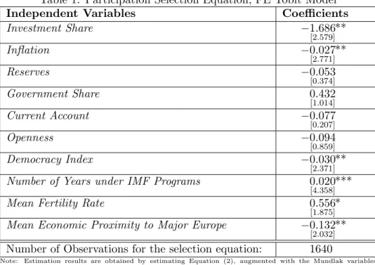
estimating Equation (2), with the full set of observations available. Table 1: Participation Selection Equation, FE Tobit Model

Independent Variables Coefficients

Investment Share −1.686 [2.579]** Inflation −0.027 [2.771]** Reserves −0.053 [0.374] Government Share 0.432 [1.014] Current Account −0.077 [0.207] Openness −0.094 [0.859] Democracy Index −0.030 [2.371]**

Number of Years under IMF Programs 0.020

[4.358]***

Mean Fertility Rate 0.556

[1.875]*

Mean Economic Proximity to Major Europe −0.132

[2.032]**

Number of Observations for the selection equation: 1640

Note: Estimation results are obtained by estimating Equation (2), augmented with the Mundlak variables capturing fixed effects. The dependent variable is the loan-quota ratio. The F-test of joint significance of the Mundlak variables is significant at the 5% significance level. t-statistics are displayed in square brackets underneath the coefficient estimates. A “*” indicates significance at the 10% level, a “**” indicates significance at the 5% level and a “***” indicates significance at the 1% level. The regression uses annual data, the sample extends from 1975 to 2005 and the number of countries considered is 68. A description of all variables used is provided in Appendix B.

As can be seen from Table 1, the estimated coefficients on the invest-ment share, inflation, measure of democracy and mean economic proxim-ity to Major Europe are significantly negative. If the investment share or the inflation rate decline by one percentage point, then the ratio of IMF lending to a country’s quota increases by 1.686 or 0.027 percentage points,

20

One of the conditioning variables, the (growth rate of the) index of institutional quality, is available only for a sub-set of the observations in our sample. When using this sub-set of observations the results of the selection equation do not change qualitatively, however.

respectively.21 If the measure for democracy increases by one basis point or the mean economic proximity to Major Europe increases by one percentage point, then the loan-quota ratio decreases by 3 or 0.132 percentage points, respectively. The effect of a country’s mean fertility rate and the number of years a country has been under IMF loan programs are significantly positive. If the mean fertility rate increases by one percentage point or the number of years under IMF loan programs increases by one year, then the loan-quota ratio increases by 0.556 and 2 percentage points, respectively.

Figure 1 displays the marginal effects (red curve) of the significant vari-ables from Table 1 as well as the corresponding one-standard deviation (green) and two-standard deviation (blue) bands.

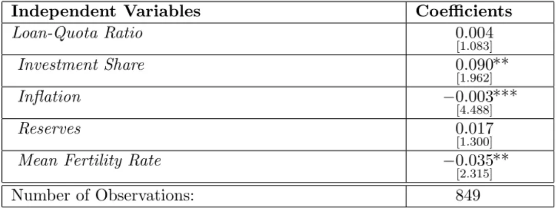
The residual obtained from estimating the participation selection equa-tion can be used to generate correcequa-tion terms that, as described in Sub-Section 3.1, in addition to correcting for sample selection also correct for endogeneity when estimating the effects of changes in the loan-quota ratio on the output growth of countries participating in IMF loan programs. Ta-ble 2 displays our estimation results for the fixed effects participation effects model (without state dependence) of Sub-Section 3.1, using the growth rate of real GDP per capita as the dependent variable and the IMF loan-quota

ratio,22 as well as a set of explanatory variables as independent variables.23

The estimated coefficient on the investment share is significantly positive. An increase of the investment share by one percentage point increases a

21

Note that differentiating the latent variable (denoted here generically as y∗) with respect to the independent variable (denoted here generically asx, entering into the Tobit model with a coefficient ofβ), we of course have

∂E(y∗|x)

∂x =β.

The marginal effect for the observed dependent variable needs to be corrected for cen-soring, multiplying β with the probability that the loan-quota ratio is strictly positive. All reported effects are average marginal effects evaluated at the independent variables’ sample means.

22

The IMF loan-quota ratio captures the average, on a monthly basis, of funds agreed upon in all loan programs (SBA, EFF, SAF, ESAF/PRGF) divided by the country’s quota at the IMF. Note that Dreher (2006) only covers those arrangements that have been active for at least five months in a given calendar year. Our results do not change if we adjust the loan-quota ratio accordingly. Similar to Vreeland (2003), we consider consecutive agreements with the IMF as part of the same spell, since governments most of the time have several consecutive agreements with the IMF. A description of all variables used is provided in Appendix B.

23_{All standard errors reported in the following tables are corrected for first-step sampling} uncertainty affecting second-step inference. See also Appendix A.

Figure 1: Marginal Effects for Participation Selection Equation

(a) Investment share (b) Inflation

(c) Democracy (d) Number of years under IMF programs

(e) Mean fertility rate (f) Mean economic proximity to Major Europe

country’s growth rate of real GDP per capita by 0.09 percentage points.

The coefficients on inflation and the mean of a country’s fertility rate are significantly negative. An increase of inflation by one percentage point and an increase of the mean fertility rate by one unit lead to a decrease of the

real GDP per capita growth rate by 0.003 and 0.035 percentage points,

respectively.

Two further issues are worth noting: First,τ1(not displayed in the table)

is significant at the 10% level, providing evidence for a sample selection mechanism. Second, the coefficient on the loan-quota ratio is positive but not significant.24

cor-Table 2: Participation Effects Equation, FE Model without State Depen-dence

Independent Variables Coefficients

Loan-Quota Ratio 0.004 [1.083] Investment Share 0.090 [1.962]** Inflation −0.003 [4.488]*** Reserves 0.017 [1.300]

Mean Fertility Rate −0.035

[2.315]**

Number of Observations: 849

Note: Estimation results are obtained by estimating Equation (1), augmented with the Mundlak variables to capture fixed effects. The F-test of joint significance of the correction terms, τ1andτ2, is not significant,

butτ1is individually significant at the 10% significance level, indicating correlation between the idiosyncratic

error terms. The dependent variable is real GDP per capita growth. t-statistics are displayed in square brackets underneath the coefficient estimates. A “*” indicates significance at the 5% level and a “**” indicates significance at the 1% level. The regression uses annual data, the sample extends from 1975 to 2005 and the number of countries considered is 68. A description of all variables used is provided in Appendix B.

To address the issue of heterogeneity bias in the loan program partici-pation effects estimates when state dependence of the effects is ignored, in our next step of analysis we condition the effects of the loan-quota ratio on output growth on the amount-drawn-to-amount-agreed ratio, which, as discussed in Section 5, may serve as a useful proxy for measuring state de-pendence of effects. Taking into account such state dede-pendence may also on its own contribute to alleviating the endogeneity problem: One may expect that a higher degree of compliance with conditionality causes higher (lower) output growth if the reforms implemented promote higher (lower) output growth. However, output growth should have a negligable effect on compli-ance with conditionality. It appears sensible to conjecture that lower output growth raises a country’s willingness to accept painful economic reforms. In this case, lower output growth should be associated with a higher degree of compliance. In any case, the amount-drawn-to-amount-agreed ratio and real GDP per capita growth in our data set feature a correlation of -0.05 only.

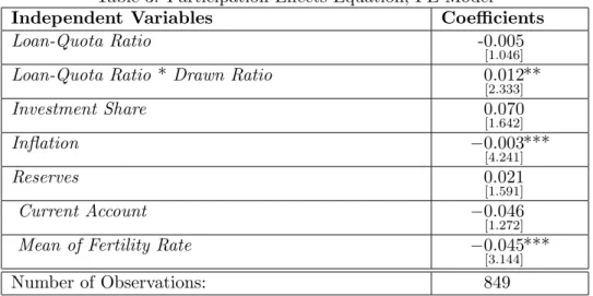
Table 3 provides our estimation results when using Chebyshev

polynomi-rection terms (which we can do for a total of 938 observations), then the coefficient on the loan-quota ratio has negative sign (−0.003), with a t-statistic of−1.522.

als of order one and the amount-drawn-to-amount-agreed ratio as capturing state dependence.

Table 3: Participation Effects Equation, FE Model

Independent Variables Coefficients

Loan-Quota Ratio -0.005

[1.046]

Loan-Quota Ratio * Drawn Ratio 0.012

[2.333]** Investment Share 0.070 [1.642] Inflation −0.003 [4.241]*** Reserves 0.021 [1.591] Current Account −0.046 [1.272]

Mean of Fertility Rate −0.045

[3.144]***

Number of Observations: 849

Note: Estimation results are obtained by estimating Equation (1), augmented with the Mundlak variables to capture fixed effects. The F-test of joint significance of the correction terms, τ1andτ2, is not significant,

butτ1is individually significant at the 10% significance level, indicating correlation between the idiosyncratic

error terms. The conditioning variable, amount-drawn-to-agreed-ratio, has been used as control variable (not displayed) and is not significant. The dependent variable is real GDP per capita growth. t-statistics are displayed in square brackets underneath the coefficient estimates. A “*” indicates significance at the 10% level, a “**” indicates significance at the 5% level and a “***” indicates significance at the 1% level. The regression uses annual data, the sample extends from 1974 to 2005 and the number of countries considered is 68. A description of all variables used is provided in Appendix B.

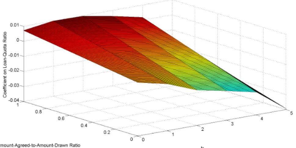
Conditioning the output growth effects of the loan-quota ratio on the proxy for compliance with conditionality has a considerable effect on the estimation results: If a participating country were not to comply with con-ditionality at all, the effect of loan program participation on output growth is negative. An increase in the loan-quota ratio by 1 percentage point low-ers the growth rate of real GDP per capita by 0.005 percentage points. (If such a country does not receive any funds from the IMF, because it does not set in effect the required reforms, the output growth effect obviously would be zero.) However, the higher the compliance ratio, the smaller in absolute terms the negative output growth effect of the loan-quota ratio. If the compliance ratio is larger than 42%, then the effect of IMF program

participation turns positive.25 If all funds originally agreed upon are drawn,

25_{Note that this ratio is sizeably smaller than in Killick (1995), who sets a threshold} value for successful IMF program implementation at 80%, arguing that this cut-off point

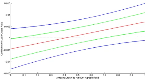
Figure 2: Effect of IMF Loan Size Conditional on Actual Degree of Program Implementation, Annual Data, 1975 - 2005, 68 Countries.

that is, there is full compliance with IMF conditionality, then an increase of the loan-quota ratio by 1 percentage point leads to an increase of real GDP per capita growth by 0.007 percentage points. These results are in line with IMF arguments stressing that compliance with conditionality is important for the success of IMF loan programs. Figure 2 plots the coefficient on the loan-quota ratio conditional on the amount-drawn-to-amount-agreed-ratio (red curve) with the one standard deviation (green) and two standard de-viation (blue) bands. The effect of the IMF loan-quota ratio at a 10% level turns significantly positive from an amount-drawn-to-amount-agreed ratio of 0.73 upwards.

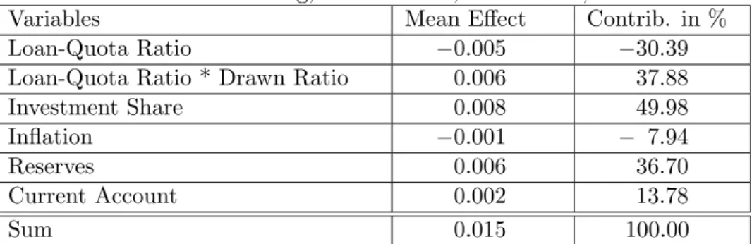
To provide a different measure of quantification of the output growth effects of IMF loan programs, Table 4 displays the average contribution of the various regressors to a country’s real GDP per capita growth net of individual-specific effects, as implied by the state-dependent panel model in Table 3:

is closely associated with successful program implementation based on a survey between 1980 and 1992.

Table 4: Growth Accounting, Annual Data, 1975 - 2005, 73 Countries.

Variables Mean Effect Contrib. in %

Loan-Quota Ratio −0.005 −30.39

Loan-Quota Ratio * Drawn Ratio 0.006 37.88

Investment Share 0.008 49.98

Inflation −0.001 − 7.94

Reserves 0.006 36.70

Current Account 0.002 13.78

Sum 0.015 100.00

The overall contribution of the loan-quota ratio to real GDP per capita

growth net of individual-specific effects is equal to 7.49%. The investment

share contributes most to a participating country’s real GDP per capita growth, at almost 50% .

To investigate the state dependence of the output growth effects of IMF program participation on a country’s institutional quality directly, we next use our index of institutional quality as described in Section 5. Since struc-tural conditionality is measured in changes by the IMF, we include the index of institutional quality in percentage changes (“institutional development”) as our conditioning variable.

Table 5 displays results when using Chebyshev polynomials of order one and institutional development as the conditioning variable.

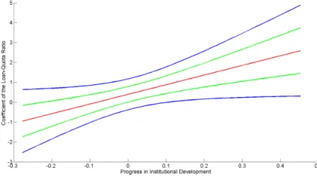
Conditioning the effect of the loan-quota ratio on institutional develop-ment yields significant results: If a country cannot improve its institutional quality, the effect of program participation on output growth is negative: An increase of the loan-quota ratio by 1 percentage point lowers the growth rate of real GDP per capita by 0.004 percentage points. At the same time, the estimated coefficient increases systematically with the magnitude of in-stitutional development. Figure 3 displays the coefficient on the loan-quota ratio conditional on the progress in institutional development. If the insti-tutional development progress exceeds 0.12, the effect of IMF loan program participation on output growth turns significantly positive at the 5% level.

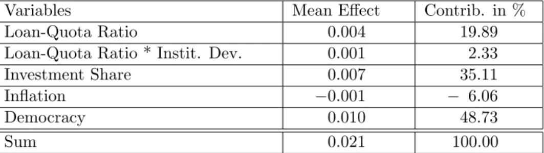
Table 6 displays the average contribution of the various regressors to a country’s real GDP per capita growth net of individual-specific effects, as implied by the state-dependent panel model in Table 5.

pro-Table 5: Participation Effects Equation, FE Model

Independent Variables Coefficients

Loan-Quota Ratio 0.004

[1.024]

Loan-Quota Ratio * Institutional Development 0.049

[2.002]** Investment Share 0.070 [0.865] Inflation −0.003 [4.257]*** Democracy 0.002 [1.059]

Mean Fertility Rate −0.038

[2.070]**

Number of Observations: 773

Note: Estimation results are obtained by estimating Equation (1), augmented with the Mundlak variables to capture fixed effects. The F-test of joint significance of the correction terms,τ1andτ2, is not significant. The

conditioning variable, institutional development, has also been considered as a control variable (not displayed) and is not significant. The dependent variable is real GDP per capita growth. t-statistics are displayed in square brackets underneath the coefficient estimates. A “*” indicates significance at the 10% level, a “**” indicates significance at the 5% level and a “***” indicates significance at the 1% level. The regression uses annual data, the sample extends from 1975 to 2005 and the number of countries considered is 60. A description of all variables used is provided in Appendix B.

grams on its output growth, we next turn our focus to analyses of coun-terfactuals and intertemporal effects involving IMF loan programs. To get an idea about the magnitude of the effect of IMF program participation on countries’ output growth, Tables 7 and 8 display counterfactual analyses for the panel models reported in Tables 3 and 5.

Table 7 reports that during participation in IMF loan programs countries between 1975 and 2005 had on average a real GDP per capita growth rate

of 0.56%. The predicted value of this growth rate using the coefficients from

the sample estimated only with country years under participation equals this

Table 6: Growth Accounting, Annual Data, 1975 - 2005, 65 Countries

Variables Mean Effect Contrib. in %

Loan-Quota Ratio 0.004 19.89

Loan-Quota Ratio * Instit. Dev. 0.001 2.33

Investment Share 0.007 35.11

Inflation −0.001 − 6.06

Democracy 0.010 48.73

Figure 3: Coefficient of Loan-Quota Ratio Conditioned on a Country’s Progress in Institutional Development, Annual Data, 1975 - 2005, 60 Coun-tries.

Table 7: Counterfactual Analysis, 1975 - 2005, Participating and Non-Participating Countries, Conditioning with the Amount-Drawn-to-Amount-Agreed Ratio, FE Specification

Country years Actuala) Predictedb) Predictedc) Predictedd)

Particip. 0.56% 0.56% 0.45% 1.40%

Non-Particip. 1.63% — 2.03% 1.63%

a) Actual average growth.

b) Coefficient estimates used to compute the counterfactual are taken from the model specification involving only country years with participation in IMF loan programs.

c) Coefficient estimates used to compute the counterfactual are taken from the model specification involving only country years with participation in IMF loan programs. The independent variable loan-quota ratio is always set to zero.

d) Coefficient estimates used to compute the counterfactual are taken from the model specification involving only country years without participation in IMF loan programs.

Table 8: Counterfactual Analysis, 1975 - 2005, Participating and Non-Participating Countries, Conditioning with the Progress in Institutional De-velopment, FE Specification

Country years Actuala) Predictedb) Predictedc) Predictedd)

Particip. 0.52% 0.52% 0.05% 1.43%

Non-Particip. 1.53% — 2.08% 1.53%

a) Actual average growth.

b) Coefficient estimates used to compute the counterfactual are taken from the model specification involving only country years with participation in IMF loan programs.

c) Coefficient estimates used to compute the counterfactual are taken from the model specification involving only country years with participation in IMF loan programs. The independent variable loan-quota ratio is always set to zero.

d) Coefficient estimates used to compute the counterfactual are taken from the model specification involving only country years without participation in IMF loan programs.

0.56%, while the fitted value using the same coefficients, but counterfactually

setting the loan-quota ratio to zero, amounts to 0.45%. The predicted value

using the coefficients from the sample estimated only with country years not

under participation amounts to 1.40%. Non-participating countries actually

had on average a real per capita GDP growth of 1.63%. The predicted

value using the coefficients from the sample estimated only with country

years not under participation amounts to 1.63% while the fitted value using

the coefficients from the sample estimated only with countryyears under participation, but counterfactually setting the loan-quota ratio always to

zero, amounts to 2.03%.

Three points are worth highlighting here. First, the second column of Table 7 highlights the fact that country years under IMF loan participation are times of (economic) crises. On average, countries had much lower output growth during years of participation in IMF loan programs. For this reason, it is imperative to properly capture the direction of causation in growth regressions involving development aid. Second, countries in economic crisis are, on average, better off when turning to the IMF and participating in

IMF loan programs. The annual percentage gain amounts to 0.11% real per

capita GDP growth per year. Nevertheless, as our results make clear, it is important for a country to comply with conditionality and improve upon its institutional quality. Third, according to our counterfactuals, countries that participated in IMF loan programs would have had an average growth

rate of 1.40% had they not participated. This number is almost three times as high as their actual average growth rate, and thus seems rather unreal-istic. Our counterfactuals thus appear to provide evidence in favor of the presumption underlying our estimation strategy that countries entering IMF loan programs in times of crises have fundamentally different growth regimes than those countries that do not.

To learn more about the dynamic effects of IMF loan-program partic-ipation on a country’s output growth, we finally turn to estimating the country’s growth rates betweent−1 andt−1 +i,i= 1,2, ...,5, that can be

attributed to IMF loan participation in yeart.26 Figures 4 and 5 display the

intertemporal effects when taking the optimal specification of the fixed ef-fects model with the amount-drawn-to-amount-agreed ratio or the progress in institutional development as conditioning state variable, respectively. Figure 4: Intertemporal Effect of the Loan-Quota Ratio on a Country’s Output Growth in the FE Model with Amount-Drawn-to-Amount-Agreed Ratio as Conditioning Variable.

Tables 9 and 10 display the corresponding coefficients and their signifi-cance levels for all time periods.

The output growth effects of participation in IMF loan programs are significant for up to three years after participation in an IMF loan program. For all time periods the output growth effects of participation in IMF loan

26

Note that it is not yet possible to use a dynamic model structure, in particular in the growth equation, in our sample selection model.

Figure 5: Intertemporal Effect of the Loan-Quota Ratio on a Country’s Output Growth in the FE Model with Progress of Institutional Development as Conditioning Variable.

Table 9: Coefficients of the Loan-Quota Ratio in the FE Model in an In-tertemporal Perspective with the Amount-Drawn-to-Amount-Agreed Ratio as Conditioning Variable

Dep. Variable Loan-Quota Ratio Loan-Quota Ratio*Drawn Ratio

yt−yt−1 yt −0_[1._.005_046] 0_[2._.012_333]** yt+1−yt−1 yt+1 −0_[0._.009_863] 0_[1._.019_923]* yt+2−yt−1 yt+2 −0_[0._.017_932] 0_[2._.026_166]** yt+3−yt−1 yt+3 −0_[0._.021_868] 0_[1._.027_809]* yt+4−yt−1 yt+4 −0_[0._.025_765] 0_[1._.027_336] yt+5−yt−1 yt+5 −0_[0._.040_832] 0_[0._.023_809]

Note: T-statistics are displayed in square brackets. A “*” indicates significance at the 10% level and a “**” indicates significance at the 5% level.

Table 10: Coefficients of the Loan-Quota Ratio in the FE Model in an Intertemporal Perspective with the Progress in Institutional Development as Conditioning Variable

Dep. Variable Loan-Quota Ratio Loan-Quota Ratio*Instit. Dev.

yt−yt−1 yt 0_[1._.004_024] 0_[2._.049_002]** yt+1−yt−1 yt+1 0_[0._.008_981] 0_[1._.060_737]* yt+2−yt−1 yt+2 0_[0._.006_401] 0_[0._.110_265] yt+3−yt−1 yt+3 0_[0._.008_372] 0_[0._.023_294] yt+4−yt−1 yt+4 0_[0._.007_265] 0_[0._.014_165] yt+5−yt−1 yt+5 −0_[0._.001_028] 0_[0._.026_333]

Note: T-statistics are displayed in square brackets. A “*” indicates significance at the 10% level and a “**” indicates significance at the 5% level.

programs are more favorable if a country complies with conditionality / improves on institutional development.

7

Conclusion

Through modelling conditionality of the output growth effects of IMF pro-gram participation, in this paper we have shed light on what appears to be a major reason as to why previous empirical studies have arrived at mixed results, ranging from positive output growth effects to no effects to nega-tive effects from IMF program participation. Allowing the effects of IMF program participation to vary systematically with the degree of program implementation or an index of institutional development, we find that there are significant positive effects of IMF program participation on a country’s output growth only if the IMF programs are implemented to a sufficient degree or if the program participation is coupled with sufficient progress in improving institutional quality.

With regards to the magnitude of these output growth effects, our growth accounting calculations provide evidence that IMF loans have a sizeable impact. Their output growth effect, in absolute size, is larger than that of inflation, for example, though much smaller than that of investment in physical capital.

participat-ing in IMF loan programs would on average have had lower output growth, had they not participated in IMF loan programs. The higher the degree of program implementation and improvement in institutional quality, the higher the potential gains from participating in IMF loan programs. We also find that output growth effects of IMF program participation are significant for up to three years after program participation, and are significantly pos-itive if participating countries comply with conditionality. Countries that decide to turn to the IMF for funding appear well advised to comply with IMF conditionality and to make every effort in improving their institutional environment.

Appendix A: Computation of Conditional

Expecta-tions and of Standard Errors

In this appendix we first discuss the computation of the conditional expec-tation in Equation (10) needed to correct the output growth equation, that is Equation (1), under the random effects specification for sample selection

bias, while also allowing for endogeneity of dit.27 The conditional

expec-tation of vit given ZZZi, dddi, and αi on the right hand side of Equation (2) is calculated as follows: E(vit|ZZZi, dddi, αi) = dit−(αi+zzz0itγγγ) 1(dit>0)−  σ_υ φ(αi+zzz0_itγγγ συ ) Φ(−αi−zzz0itγγγ συ )  1_(dit=0),(23)

whereφand Φ denote the standard normal probability and cumulative

den-sity functions, respectively, and 1(·) denotes the indicator function.

Using this expression, the conditional expectation ofuitgivenZZZi anddddi, Equation (10), can be obtained as:

E[uit|ZZZi, dddi] = Z    αi+ dit−(αi+zzz0itγγγ) 1_(dit>0)−συ φ(αi+zzz0itγγγ συ ) Φ(−αi−zzz 0 itγγγ συ ) 1_(dit=0)    · h QT t=1Φ( −αi−zzz0itγγγ συ )1(dit=0) 1 συφ( dit−αi−zzz0itγγγ συ )1(dit>0) i 1 σαφ( αi σα) R hQT t=1Φ( −αi−zzz0itγγγ συ )1(dit=0) 1 συφ( dit−αi−zzz0itγγγ συ )1(dit>0) i 1 σαφ( αi σα)dαi dαi. (24) When obtaining standard errors for the estimates of the parameters of the output growth equation under the two-step procedure of Section 3, the sampling uncertainty that has entered the construction of the correction

factors ˆuit and ˆu¯i needs to be observed. The following estimator of the

variance-covariance matrix ofπππ = (θ βββ0 τ1 τ2)0 reflects this sampling

uncer-tainty: ˆ V arN = 1 N ˆ G GG−_N1 ˆ V VVN + ˆDDDNWWWˆNDDDˆ 0 N ˆ G GG−_N1, (25)

27_{Note that the conditional expectation E(˜u}

it|ZZZi, dddi) arising under the fixed effects

specification can be computed in analogous fashion, and thus need not be considered separately.

where ˆWWWN =V arˆ N(ˆγγγ), ˆ G GGN = 1 N N X i=1 RRR0_iRRRi, (26) ˆ V VVN = 1 N N X i=1 R RR0_ieeeˆieeeˆ0iRRRi, (27) ˆ DDDN = 1 N N X i=1 R RR0_i∂ (ˆuuuiuˆ¯iιιι) ˆτττ ∂γγγ _{γγγ=ˆγγγ}, (28) with R RRi = dddixxx0iuuˆui uˆ¯iιιι , (29) τττ = (τ1 τ2)0, (30)

andιιιis again a vector of ones of size Ti. Note that if τ2 = 0 is imposed in

the estimation, then it appears sensible to also impose that ˆeeeiˆeee0i is a diagonal

matrix (reflecting thateit is restricted to be intertemporally uncorrelated).

Computation of the standard errors of the growth equation parameter estimates under the fixed effects specification can proceed in analogy to Equations (25) and (30).

Appendix B: Description of Variables

Variables Source

Real GDP per capita: International Dollar in 2000 Constant Prices, thousand

dollars.

Penn World Tables 6.2

Openness in constant prices: Percentage in 2000 constant prices. Penn World Tables 6.2

Government share of real GDP: Percentage in 2000 Constant prices. Penn World Tables 6.2

Investment share of real GDP: Percentage in 2000 Constant prices. Penn World Tables 6.2

Total reserves in months of imports: Amount of reserves in terms of the

number of months of imports of goods and services which can be paid.

World Development Indi-cators 2006 CD-ROM

Inflation: Annual percentage change of the consumer price index. World Development

Indi-cators 2006 CD-ROM

Life expectancy at birth: Expresses the number of years a newborn can be

expected to live if prevailing patterns of mortality at the time of its birth are same throughout its life.

World Development Indi-cators 2006 CD-ROM

Fertility rate: Number of children that are born to a woman if she lives to

the end of her childbearing years and bears children in accordance with current age-specific fertility rates.

World Development Indi-cators 2006 CD-ROM

Economic proximity to major Europe: Bilateral trade with major Europe,

expressed as a ratio to GDP.

Barro and Lee (2005)

Political proximity to major Europe: Fraction of UN votes along with major

Europe.

Barro and Lee (2005)

Democracy index: Based of the Legal Index of Electoral Competitiveness

(LIEC); Codified with 1 if it has a value of 6 or larger which is the threshold for democratic systems.

World Bank Political Insti-tutions Dataset

Quota: Countries’ quota in millions of standard drawing rights (SDR). International Financial

Statistics

Loan-quota ratio: Sum of all current IMF loans a country is eligible to as a

share of its quota at the IMF.

International Financial Statistics and own calcu-lation

Amount-drawn-to-amount-agreed ratio: The amount of all IMF loan

pro-gram funds a country actually draws expressed as a share of the original amount agreed upon with the IMF.

International Financial Statistics and own calcu-lations

Government Stability: Assesses the government’s ability to carry out its

de-clared program(s), and its ability to stay in office.

International Country Risk Guide

Internal Conflict: Assesses the political violence in the country and its actual

or potential impact on governance.

International Country Risk Guide

Corruption: Assesses corruption within the political system. International Country

Risk Guide

Law and Order: Assesses the strength and impartiality of the legal system as

well as the popular observance of the law.

International Country Risk Guide

Ethnic Tensions: Assesses the degree of tension within a country attributable

to racial, nationality, or language divisions.

International Country Risk Guide

Bureaucracy Quality: Assesses the institutional strength and quality of the

bureaucracy.

International Country Risk Guide

Educational attainment: Total population aged 15 and over, average years of

school.

Worldbank

Institutional Index: Set up from the variables educational attainment, life

ex-pectancy, government stability, bureaucracy quality, corruption, law and order, ethnic tensions and internal conflict

International Country Risk Guide and own calculations

Freedom Status: Assesses political rights and civil liberties in a country. Freedom House

Appendix C: Countries Contained in Data Set

Country Start :

end of

sample

Years with Program Partici-pation

Country Start :

end of

sample

Years with Program Partici-pation Algeria 1977:1991 1989:1991 Liberia 1979:1987 1979:1985 Argentina 1976:2004 1976:1978; 1983:2004 Madagascar 1975:2003 1977:1978; 1980:1992; 1996:2003 Australia 1975:2004 % Malawi 1981:2002 1981:1986; 1988:2002 Austria 1975:2004 % Malaysia 1975:2003 % Bangladesh 1987:2003 1987:1993; 2003:2003 Mali 1989:2003 1989:2003 Belgium 1975:2001 % Mexico 1979:2004 1979:1979; 1983:1993; 1995:1997; 1999:2000 Bolivia 1976:2003 1980:1980; 1986:2003 Morocco 1975:2003 1980:1993 Botswana 1976:2003 % Mozambique 1988:2003 1988:2003 Brazil 1981:2003 1983:1986; 1988:1990; 1992:1993; 1998:2003 Namibia 2003:2003 %

Burkina Faso 1975:2001 1991:2001 Netherlands 1975:2004 %

Cameroon 1977:1995 1988:1992; 1994:1995 New Zealand 1975:2004 %

Canada 1975:2004 % Nicaragua 1977:2004 1979:1979; 1991:2004

Chile 1975:2004 1975:1976; 1983:1990 Niger 1975:2003 1983:1991; 1994:2003

Colombia 1975:2003 1999:2003 Nigeria 1977:2004 1987:1987; 1989:1992; 2000:2001

Congo, Rep. 1986:2003 1986:1988;1990:1992; 1994:1999 Norway 1975:2004 %

Costa Rica 1977:2004 1977:1977; 1980:1983; 1985:1997 Pakistan 1976:2004 1977:1978; 1980:1983; 1988:1991;

1993:2004

Cote d’Ivoire 1975:2003 1981:1992; 1994:2003 Panama 1977:2003 1977:1987; 1992:2002

Cyprus 1976:2004 1980:1981 Papua New

Guinea 1976:2001 1990:1992; 1995:1997; 2000:2001 Denmark 1975:2004 % Paraguay 1975:2003 2003:2003 Dominican Re-public 1975:2003 1983:1986; 1991:1994; 2003:2003 Peru 1977:2003 1977:1980; 1982:1985; 1993:2003 Ecuador 1976:2004 1983:1992; 1994:1995; 2000:2001; 2003:2004 Philippines 1977:2004 1977:1981; 1983:2000

Egypt, Arab Rep. 1977:2003 1977:1981; 1987:1988; 1991:1998 Portugal 1976:2004 1977:1979; 1983:1985

El Salvador 1976:2003 1980:1983; 1990:2000 Senegal 1975:2003 1979:1992; 1994:2003

Finland 1975:2004 1975:1976 Sierra Leone 1977:2003 1977:1982; 1984:1989; 1994:1998;

2001:2003

France 1975:2004 % Singapore 1975:2004 %

Gambia, The 1978:1997 1978:1980; 1982:1991 South Africa 1975:2004 1976:1977; 1982:1983

Germany 1992:2004 % Spain 1975:2004 1978:1979

Ghana 1975:2003 1979:1979; 1983:1992; 1995:2003 Sri Lanka 1975:2003 1975:1975; 1977:1981; 1983:1984;

1988:1995; 2001:2003

Greece 1976:2004 % Sudan 1977:2003 1979:1985

Guatemala 1977:2003 1981:1984; 1988:1990; 1992:1994;

2002:2003

Sweden 1975:2004 %

Guinea-Bissau 1988:2003 1988:1990; 1995:1998; 2000:2003 Syrian Arab Rep. 1977:1988 %

Haiti 1975:2000 1975:1990; 1995:1999 Thailand 1975:2003 1978:1979; 1981:1983; 1985:1986;

1997:2000

Honduras 1975:2004 1979:1983; 1990:1997; 1999:2002;

2004:2004

Togo 1975:2003 1979:1998

India 1975:2003 1981:1984; 1991:1993 Trinidad and

To-bago

1975:2003 1989:1991

Indonesia 1981:2004 1997:2003 Tunisia 1984:2004 1986:1992

Ireland 1975:2004 % Turkey 1975:2004 1978:1985; 1994:1996; 1999:2004

Israel 1975:2004 1975:1977 Uganda 1981:2003 1981:1984; 1987:2003

Italy 1975:2004 1975:1975; 1977:1978 United Kingdom 1975:2004 1975:1978

Jamaica 1976:2003 1977:1996 United States 1975:2004 %

Japan 1977:2004 % Uruguay 1978:2004 1978:1987; 1990:1993; 1996:2004

Jordan 1975:2003 1989:1990; 1992:2003 Venezuela, RB 1975:2004 1989:1993; 1996:1997

Kenya 1975:2003 1975:1986; 1988:1994; 1996:2003 Zambia 1986:2000 1986:1987,1995:2000

Korea, Rep. 1976:2004 1976:1977; 1980:1987; 1997:2000 Zimbabwe 1980:1994 1981:1984; 1992:1994

28

Major oil exporting countries, centrally planned and island economies have been ex-cluded.

Appendix D: Results for the Random Effects Panel

Model

Table 12: Participation Selection Equation, RE Tobit Model

Independent Variables Coefficients

Investment Share −1.174 [4.013]*** Inflation −0.016 [2.798]** Government Share 0.513 [2.359]**

Number of Years under IMF Programs 0.021

[7.562]***

Staffshare at IMF −0.029

[1.630]

Political Proximity to Major Europe −0.123

[2.682]** Reserves −0.047 [0.692] Current Account −0.173 [0.903] Openness −0.123 [2.257]** Democracy −0.013 [1.967]**

Number of Observations for the selection equation: 2439

Note: Estimation results are obtained by estimating Equation (2). The dependent variable is the loan-quota ratio. t-statistics are displayed in square brackets underneath the coefficient estimates. A “*” indicates significance at the 10% level, a “**” indicates significance at the 5% level and a “***” indicates significance at the 1% level. The regression uses annual data, the sample extends from 1975 to 2005 and the number of countries considered is 73. A description of all variables used is provided in Appendix B.

Figure 6: Effect of IMF Loan Size Conditional on Actual Degree of Program Implementation, Annual Data, 1975 - 2005, 73 Countries.

Figure 7: Coefficient of Loan-Quota Ratio Conditioned on a Country’s Progress in Institutional Development, Annual Data, 1975 - 2005, 65 Coun-tries.

Figure 8: Intertemporal Effect of the Loan-Quota Ratio on a Country’s Output Growth in the RE Model with Amount-Drawn-to-Amount-Agreed Ratio as Conditioning Variable.

Figure 9: Intertemporal Effect of the Loan-Quota Ratio on a Country’s Out-put Growth in the RE Model with the Progress in Institutional Development as Conditioning Variable.