Data-driven fMRI data analysis based on parcellation

Ji, Yongnan (2001) Data-driven fMRI data analysis

based on parcellation. PhD thesis, University of

Nottingham.

Access from the University of Nottingham repository: http://eprints.nottingham.ac.uk/12645/1/546702.pdf

Copyright and reuse:

The Nottingham ePrints service makes this work by researchers of the University of Nottingham available open access under the following conditions.

· Copyright and all moral rights to the version of the paper presented here belong to the individual author(s) and/or other copyright owners.

· To the extent reasonable and practicable the material made available in Nottingham ePrints has been checked for eligibility before being made available.

· Copies of full items can be used for personal research or study, educational, or not-for-profit purposes without prior permission or charge provided that the authors, title and full bibliographic details are credited, a hyperlink and/or URL is given for the original metadata page and the content is not changed in any way.

· Quotations or similar reproductions must be sufficiently acknowledged. Please see our full end user licence at:

http://eprints.nottingham.ac.uk/end_user_agreement.pdf A note on versions:

The version presented here may differ from the published version or from the version of record. If you wish to cite this item you are advised to consult the publisher’s version. Please see the repository url above for details on accessing the published version and note that access may require a subscription.

Data-driven fMRI data analysis based on

parcellation.

YongnanJiMSc.

Thesis submitted to The University of Nottingham

for the degree of Doctor of Philosophy

... I

The University of

ｾ

I

Nottingham

School of Computer Sciences

University of Nottingham

Abstract

Functional Magnetic Resonance Imaging (fMRI) is one of the most popular neu-roimaging methods for investigating the activity of the human brain during cogni-tive tasks. As with many other neuroiroaging tools, the group analysis of fMRI data often requires a transformation of the individual datasets to a common stereotaxic space, where the different brains have a similar global shape and size. However, the local inaccuracy of this procedure gives rise to a series of issues including a lack of true anatomical correspondence and a loss of subject specific activations.

Inter-subject parcellation of fMRI data has been proposed as a means to alleviate these problems. Within this frame, the inter-subject correspondence is achieved by isolating homologous functional parcels across individuals, rather than by match-ing voxels coordinates within a stereotaxic space. However, the large majority of parcellation methods still suffer from a number of shortcomings owing to their de-pendence on a general linear model. Indeed, for all its appeal, a GLM-based parcel-lation approach introduces its own biases in the form of a priori knowledge about such matters as the shape of the Hemodynamic Response Function (HRF) and task-related signal changes.

In this thesis, we propose a model-free data-driven parcellation approach to single-and multi-subject parcellation. By modelling brain activation without an relying on an a priori model, parcellation is optimized for each individual subject. In order to establish correspondences of parcels across different subjects, we cast this problem as a multipartite graph partitioning task. Parcels are considered as the vertices of a weighted complete multipartite graph. Cross subject parcel matching becomes equivalent to partitioning this graph into disjoint cliques with one and only one parcel from each subject in each clique. In order to solve this NP-hard problem, we present three methods: the OBSA algorithm, a method with quadratic program-ming and an intuitive approach. We also introduce two quantitative measures of the quality of parcellation results.

We apply our framework to two fMRI data sets and show that both our single- and multi-subject parcellation techniques rival or outperform model-based methods in terms of parcellation accuracy.

Acknowledgem.ents

I would like to thank my supervisor Dr. Alain Pitiot. Without his help I would not have had the opportunity to focus on this subject. I would also like to thank Profes-sor Uwe Aickelin for his support and guidance. Additionally, I want to express my thanks to Dr. Pierre-Yves Herve for his suggestions and advice.

Thanks also go to the committee of Collaborative Medical Image Analysis On Grid (CMIAG) group. I have been fortunate to receive funding from Marie Curie Action to complete the research. I also deeply appreciate the help I have received from the School of Computer Science, Brain & Body Centre and School of Psychology in the University of Nottingham.

Lastly but certainly not least, I would like to thank my family for their support over the years. I would especially like to thank my wife Xiaojie Song. Without her en-couragement and support I would not have been able to concentrate and complete this thesis.

Contents

1 Introduction

1.1 Background and motivation 1.2 Aim and contribution .

1.3 Overview of the thesis

2 Literature Review

2.1 Introduction to fMRI

2.2 fMRI data analysis .

2.2.1

2.2.2

2.2.3

2.2.4

Preprocessing of fMRI data General Linear Model . . . Data-Driven analyses (DDA)

Machine learning classifier for fMRI data analysis

2.3 Human Brain Parcellation . .

2.3.1 Top-down approaches 1 1 7 9 11 11 14

15

25

CONTENTS

2.3.2 Bottom-up approaches .

2.4 Summary...

3 Parcellation of Individual Subjects

3.1 3.2

Introduction . . . . Feature extraction for parcellation

3.2.1 Histogram of functional images

40 42 44 44 46 48

3.2.2 Independent Components Analysis for fMRI Group Analysis 50

3.2.3 3.2.4 3.2.5

Seed Selection . . . . PCA for fMRI denoising .

Partial Least Square (PLS) for feature extraction 3.3 Spatially constrained clustering for parcellation .

3.3.1 3.3.2 3.3.3

Clustering on the manifold for parcellation Aggregation and Boundary Competition Discussion . . . .

3.4 Validation of Intra-subject Parcellation 3.4.1

3.4.2 3.4.3

Intra-parcel functional variance . Nearest Silhouette Coefficient . Results from the toy data 3.5 Summary... 53 54 58

59

CONTENTS

4 Cross Subject Comparison of Parcels 4.1 Introduction . . . . 4.2 Multi-subject parcellation

96 96 98 4.3 Cross-subject matching as a multipartite graph partitioning problem 100

4.4

4.5

4.3.1 Multipartite graph partitioning for cross-subject matching 100

4.3.2 4.3.3

Order Based Simulate Annealing (OBSA) Bags of Pixels and Bags of Parcels . . . .

104

108

4.3.4 Quadratic programming for multipartite graph partitioning 111

Experiment results . . . . 4.4.1

4.4.2

Results from toy data .

Results from multi-subject fMRI data Discussion . . . .

113 113 119 120

5 Application to fMRI data sets 123

123 124 124 125

128

5.1

5.2

Experiment on single-subject motor cortex stimulation data

5.2.1

Experiment on multi-subject face and gesture data .

CONTENTS

5.3.2

5.3.3

Parcellation .. Result analysis

5.4 Cross-Subject parcel matching.

5.5 Summary . . . .

6 Conclusion and Future Work 6.1 Summary ..

6.2 Future Work

Further improvement to single-subject parceilation 6.2.1

6.2.2

6.2.3

Cross-subject parcel matching . Application 6.3 Closing Comment . References 143 146 151 155 158 158

165

169

List of Figures

1.1 An example of mis-registration.

1.2 Data-driven parcellation framework. . 1.3 Single subject data-driven parcellation.

2.1 Slice-timing correction for fMRI data. . . . . .

5 7 8

16

2.2 One slice of functional image, structural image and MNI atlas. 20

2.3 Process of constructing a machine learning classifier.. . . 34

3.1 3.2

A data-driven approach to parcellation. Histogram of normalized fMRI images. 3.3 Histogram filtering. . . .

3.4 Variance explained by each principal component.

3.5

3.6

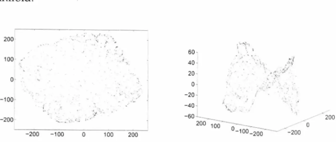
First six principal components. Last six principal components. 3.7 Distance on manifold. . . . 45 49

50

57

57

61

LIST OF FIGURES

3.8 Toy data embedded with Isomap . . . . . 3.9 Toy data embedded with Diffusion Map . 3.10 First three diffusion coordinates when 52

=

66 69

71

3.11 Illustration of noise level on the manifold of a GLM parameter map. 72

3.12 Parcellation results from toy data in different embedded spaces 73

3.12.1 The spectrum of Isomap . . . 73

3.12.2Parcellation result with first two embedded dimensions 73

3.12.3Parcellation result with first three embedded dimensions 73

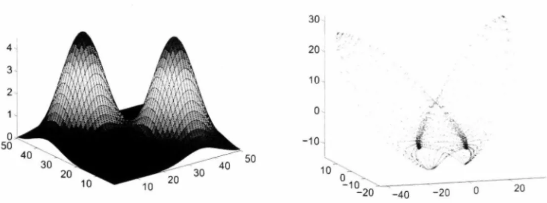
3.12.4Parcellation result with first eight embedded dimensions . 73

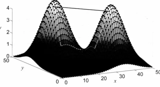
3.13 Parcellation results from toy data with noise 3.13.1 The double Gaussian data with noise 3.13.2The spectrum of Isomap . . . .

74 74 74

3.13.3Parcellation result with first two embedded dimensions 74

3.13.4Parcellation result with first eight embedded dimensions. 74

3.14 Embeddings of the toy data with noise .. 3.14.1Embedding on 2-dimensional space 3.14.2Embedding on 3-dimensional space 3.15 Embeddings of the toy data with noise ..

3.15.1Embedding on 3-dim.ensional space with 52

=

=

75 75 75 76 76 76

LIST OF FIGURES

3.16 Embeddings of the toy data with noise. 3.16.1Swiss Roll data . . . .

3.16.2Swiss Roll data with noise. 3.17 Smoothing of Swiss Roll data . . .

3.17.1 The cross validation Error .. 3.17.2Smoothing result with (!

=

3.17.3Smoothing result with (! = 1.9.

3.17.4Smoothing result with (!

=

3.18 Results of tests on Swiss Roll data ..

3.18.1Cost function for noiseless Swiss Roll data. 3.18.2Cost function for Swiss Roll data with noise. 3.18.3Cost function for smoothed noisy Swiss Roll data. 3.18.4The embedding of smoothed data

3.19 Toy data with different levels of noise. 3.20 Toy data with different levels of noise.

3.21 Embedding and parcellation on smoothed data.

3.22 Results of Aggregation (left) and Boundary Competition 3.23 Comparison of parcellation results. .

3.23.1Intra-parcel variances . . . 3.23.2Nearest Silhouette Coefficients

78 78 78 79 79 79 79 79 80 80 80 80 80 82 83 83 87 93 93 93

LIST OF FIGURES

4.1 Munkres Algorithm.

4.2 Toy data. . . .

4.3 The parcellation of the toy data ..

4.4 Comparison of parcel matching methods with toy data. 4.4.1 Matching with OBSA. . . .

4.4.2 Matching with each subject as reference. 4.5 Matched parcels. . . . . . 105 114 115 116 116 116 118

4.6 Comparison of parcel matching methods with multi-subject fMRI data. 121 4.6.1 Matching with OBSA. . . .

4.6.2 Matching with each subject as reference.

121 121

5.1 The fMRI scan of the single-subject motor cortex stimulation data. 125

5.2 Comparison of GLM t-values with and without PCA denoising. 126

5.3 Statistical maps (t

>

5.4.1 The PLS latent variable . . . . 5.4.2 GLM t-values against PLS t-values.

5.5 Parcellation results comparison with four different criteria. 5.5.1 Comparison with GLM t-values.

5.5.2 Comparison with PLS t-values ..

5.5.3 Comparison with GLM parameter

f3.

127 130 130 130 132 132 132 132

LIST OF FIGURES

5.5.4 Comparison with PLS correlation coefficient r.

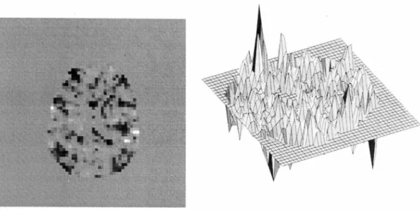
5.6 Parcellation results comparison with NSC. 5.6.1 Image of GLM parameters. . . . 5.6.2 Image of PLS correlation coefficients. 5.6.3 Histogram of GLM parameters

f3. ..

5.7.1 Comparison with GLM t-values. 5.7.2 Comparison with PLS t-values .. 5.7.3 Comparison with GLM parameter

f3.

5.7.4 Comparison with PLS correlation coefficient r.

132 137 137 137 137 137 139 139 139 139 139 5.8 Convolutional HRF model for the multi-subject face and gesture data. 142 5.9 PCA analysis of pooled ICs. . . .. 144 5.10 The dendrogram of hierarchical clustering the ICs from all subjects. 144 5.11 ICs in different clusters.

5.11.1An IC in Cluster 1. 5.11.2An IC in Cluster 2.

5.12 The clustering of ICs based on manifold ..

5.13 Comparison of functional intra-parcel homogeneity. 5.14 Comparison of parcellation results with NSC. . . . .

145 145 145 146 147 149

LIST OF FIGURES

5.15 Two types of group analysis for the 'angry hand gesture' stimulation. 153

5.16 The sum of weights of the matched parcels. 15-1

CHAPTER

1

Introduction

1.1 Background and motivation

Due to the fact that neurons do not store energy, the firing of neurons leads to changes in both local blood flow and local deoxyhemoglobin content in the blood. The dynamic regulation of the blood flow in the brain is called hemodynamic. The use of magnetic resonance (MR) scans to measure hemodynamic responses provides a non-invasive approach to study the functions of the human brain.

The hemodynamic response corresponding to neural activity -in the brain alters the contrast of T2* weighted magnetic resonance images (MRI) [Ogawa et al., 1990a,b; Turner et al., 1991]. This is called Blood Oxygen Level Dependence (BOLD). The precise nature of the relationship between neural activity and the BOLD signal is still a subject of research. However, in general, they are well related. Functional Magnetic Resonance Imaging (fMRI) uses BOLD signals as an indirect approach to the measurement of neural activity in the brain.

CHAPTER 1: INTRODUCTION

The use of fMRI to measure BOLD signals has provided neuroscientists with a pow-erful tool to examine brain activity. It has been widely used in various fields of neuroscience [Achard et a1., 2006; Cohen et a1., 2008; Simon et a1., 2004]. As the ac-quisition of fMRI signals is complicated and BOLD signals have a very low signal-noise-ratio, preprocessing is an important step for fMRI data analysis.

According to different research aims, many methods have been proposed for fMRI data analysis. The General Linear Model (GLM) introduced by Friston et a1. [1994] is one of the most popular model-driven methods in fMRI data analysis. In this re-gression method, a model is first set up to describe the BOLD signals corresponding to the stimulation, after which the model is applied to the data. Statistical analysis is performed on each voxel with the null hypothesis that the model does not match the time course on that voxe1. Therefore, for each voxel, GLM provides a statisti-cal measure (e.g. a t-value or an F-value) to present the possibility that the brain structure corresponding to that voxel is activated during the stimulation.

In GLM-based analysis, the shapes of the BOLD responses are presumed to be the same for all subjects and voxels. The variability of the BOLD responses is ignored. However, as shown by Aguirre et a1. [1998] and Handwerker et a1. [2004], the BOLD responses of the human brain vary across subjects, trials, days, and even different regions in the brain. Therefore, several methods have been proposed to overcome the int1uence of BOLD variability in model-driven study. For instance, Friston et a1. [1999]; Woolrich et a1. [2004] have proposed different basis sets for the Hemody-namic Response Function (HRF). The authors first define an HRF basis set, which could describe the reasonable HRF 5hapes. The BOLD signals from different subjects

CHAPTER 1: INTRODUCTION

can be modelled with different HRFs from the predefined basis set. These methods relax the assumption of BOLD signals from a fixed model to a model set.

Some other analysis methods do not require the assumption about the shapes of BOLD. For instance, Backfrieder et al. [1996] use Principal COII).ponent Analysis (PCA) for fMRI data analysis. With visual and motor stimulation experiments, they show that their method yields accurate absolute quantification of in vivo brain activity. Besides PCA, McIntosh et al. [2004] have proposed Partial Least Squares (PLS) as an effective multivariate analytic tool to identify brain activity patterns. In this work, they use event-related fMRI data to demonstrate that their method could provide robust statistical assessment without making assumptions about the shape of the HRFs.

Data-driven analysis is another type of method widely used in the area of fMRI data processing, in which brain activation is detected using only information con-tained in the fMRI signal itself. Techniques, such as Independent Component Anal-ysis (ICA) [Beckmann and Smith, 2004; Li et al., 2007; Wang and Peterson, 2008] and clustering [Gao and Yee, 2003; Goutte et al., 1999], have been successfully used to ex-tract the main components of responses from the fMRI time series. As for most data-driven techniques, the components· of activation are extracted individually from each subject; the cross-subject variability of the BOLD signals does not influence the analysis results. Therefore, data-driven approaches can also be considered to be a means of solving the problem of cross-subject HRF variability.

In recent years, pattern-based classification analyses appear with increasing fre-quency in the functional neuroimaging area [Haynes et al., 2007; Kamitani and Tong,

CHAPTER 1: INTRODUCTION

2005, 2006; Mitchell et al., 2004]. These methods use machine learning algorithms to decode different mental states, behaviour and other variables from fMRI data. Compared with other methods, a machine learning classifier is complex to imple-ment but, it makes a fundamental advance in the state of the art by linking patterns of brain activity to experiment design variables [O'Toole et al., 2007].

No matter which analysis approach is used, the study of therelationship between function and structure in the human brain relies on the analysis of groups of sub-jects. Therefore, voxel-based spatial normalization is also required for multi-subject analysis in order to bring fMRI images of different subjects into the same coor-dinate system, such as Talairach space [Talairach and Tournoux, 1988] and MNI space [Evans et al., 1993]. After spatial normalization, it is generally assumed that for all subjects registered to the standard space, the same coordinates correspond to the same brain structure. Further analysis can be applied in the standard space.

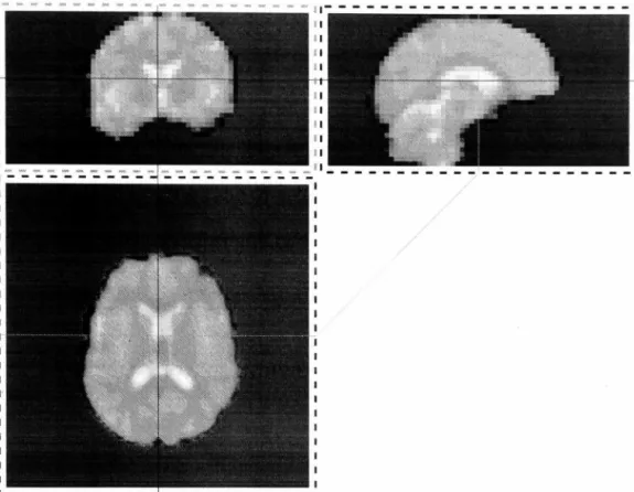
This method relies heavily on the assumption that for all spatially normalized sub-jects, the same coordinates in the standard space correspond to brain structure with the same function. However, even though many registration methods have been introduced [Brown, 1992; Zitova, 2003], due to the limitation of algorithms and the complexity of human brain anatomy, the problem of mis-registration still exists. For instance, in Figure 1.1, images from two subjects were registered to MNI space with rigid and affine registration. Both of these subjects were scanned under the same stimulation paradigm. Slice timing correction and motion correction were applied to the data. Then, the fMRI data was processed "vith GLM. The images in the red, green and blue dashed line rectangles are the images of the transverse, coronal and

CH APTER 1: INTROD U CTION -_ ... -- ---... ... ---_ ... -_ ... -_ ... ... . , ｾ Ｍ Ｍ Ｍ Ｍ Ｍ Ｍ Ｍ Ｍ Ｍ Ｍ Ｍ Ｍ Ｍ Ｍ Ｍ Ｍ Ｍ Ｍ Ｍ Ｍ Ｍ Ｍ Ｍ Ｍ Ｍ Ｍ Ｍ Ｍ Ｍ Ｍ Ｍ Ｍ Ｍ _ _ _ _ _ _ I 1.5 -1 -3.5 Legend 1 ', 11 .8125 1 8.84375 1 5.875 . 2.90625

1

Figure 1.1: An example of mis-regish-ation. The fMRl images of b oth subjects were scanned under the same stimulation paradigm. Activation w ith p

<

sec-tion 2.2.1. M ore d etails of the experiment are presented in Chapter 5

,

,

sagittal planes. In each dashed line rectangle there are two images. The left is from subject 1 and the right is from subject 2. The activation detected in subject 1 is pre-sen ted on the red and yellow t-value map as shown in legend 1. The activa tion detected in subject 2 is presented on the blue and green t-value map as show n in legend 2. Comparing the activ ation maps from both subjects on the right occipi-tal gyrus, the activation of the subject 1 is about Smm posterior to the activation in subject 2. In these two subjects, the same coordinates in the standard space d o no t correspond to the same fur'.Ction . If the activ ation regions are smail, this activation may b e missed in a group analy sis.

CHAPTER 1: INTRODUCTION

problem and overcome the limitation of spatial normalization. The parcellation of the human cerebral cortex into functionally distinct areas is an important area of neuroscience. Brodmann has parcellated the human brain into 52 different fields, based upon its cytoarchitecture. Using modem neuroimaging techniques, many methods have been proposed to parcellate the brain noninvasively[Peltier et al., 2009; Pohl, 2005; Shen et al., 2010].

Coulon et al. [2000] have proposed a method that uses hierarchical grey-level blobs to describe individual activation maps in terms of structures. A comparison graph is constructed based on these blobs for group analysis. This method can be consid-ered as one of the earliest studies to use parcellation for the analysis of functional activation maps. Later, Flandin et al. [2002] presented parcellation as a way of deal-ing with the shortcomdeal-ings of spatial normalization for model-driven analysis. They parcellate the brain of each subject into about 1000 functionally homogenous parcels with GLM parameters and group analysis is implemented on the parcels. However, this method is specifically designed for GLM analysis.

We consider that parcellation based analysis can be improved in the following two ways at least. (1) For individual subject parcellation, we need to overcome the vari-ability of HRFs and provide the parcellation that is optimised for each individual subject. So t.hat the parcellation accuracy could be increased. (2) We need to widen the scope of parcellation based analysis, so that data-driven analysis or machine learning classifiers can also be constructed on the parcels.

CHAPTER 1: INTRODUCTION

1.2 Aim and contribution

Image time-series

!

Rea linn r .. H:u·u

Data-Driven Parcellation

Cross-subject I

i parcel matching

I

!

Figure 1.2: Data-driven parcellation framework.

The aim of this research is to develop a flexible fMRI data analysis framework based on parcellation. This framework should be able cope with the problem of mis-registration and HRF variability and can be used for data-driven analysis and machine learning based analysis.

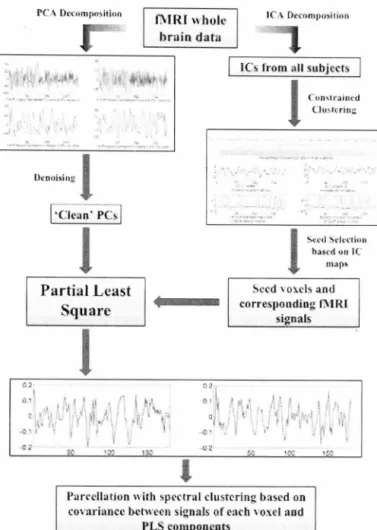
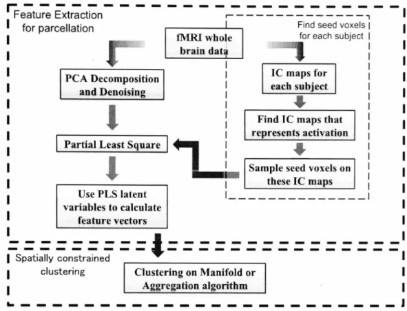
Figure 1.2 shows this framework. In order to alleviate the issue of cross-subject par-cel matching, images of all subjects are first aligned into standard space. After that a novel data-driven parcellation method based on adaptive smoothing for manifold embedding is applied to each subject [Ji et al., 2009] . Figure 1.3 shows the data flow of this method. Because no prior information on HRF is required in this approach, the cross-subject variability of HRF does not influence the parcellation results.

CHAPTER 1: INTRODUCTION ｾＮ ... ＬｾＬ ... Ｂｖｾﾷ｟Ｂ Ｇﾷ ﾷ ﾷＢ Ｂ ＧｾＢ Ｇ Ｇ Ｇ ＧｾＧ Ｇ

-,

:l

,;' ,} ,:::

----

J

J

J

ICs from all subj ects

, " . • ·"v . . ; . Ｎ Ｎ Ｎ Ｎ［ｾ ' ..

J

ｃ

ｾ

Ｇ

ｬ

ｲ

｡ ｬ

ｴ

､

J

Seed yowls and corresponding fMRI

signals

.ParceUation with spl'Ctral clustering ｢ ｡ ｳ ｾ､ on covarinnc.c between signals of each voxeJ and

PLS componcuts

Figure 1.3: Single subject data-driven parcellation.

answer the question that, given only a suitable definition of the similarity between parcels from different subjects, is it possible to use the group information to find the best parcel correspondence? In order to answer this question, we formalize the

problem of parcel matching as a multi-partite graph partitioning problem. Match-ing the parcels across all subjects is the same as partitionMatch-ing a weighted graph into disjoint cliques by cutting some edges. The matching is optimized by minimiz-ing the weights of the cut edges. We propose an order-based annealminimiz-ing method to solve this problem effectively and we discuss the similarity betw een the parcel matching problem a..."1d permutation invariant analysis Uebara, 2003] . Therefore, in

CHAPTER 1: INTRODUCTION

into quadratic programming. We test the parcel matching algorithms with one toy dataset and one fMRI real dataset.

Hypothesis

The main hypothesis of this thesis is that our multi-subject data-driven parcellation approach improves over (1) standard voxel-wise fMRl analysis in terms of both ro-bustness and sensitivity to normalization issues and (2) model-based parcellation techniques in terms of parcellation accuracy.

1.3 Overview of the thesis

Chapter 2 presents a review of the related work on fMRl data analysis and par-cellation. We discuss previous work on model-driven and data-driven fMRl data analysis. Moreover, the problems of mis-registration and variability of HRF are ad-dressed in this chapter.

Then, in Chapter 3, we first discuss spectral clustering and its application to par-cellation. Next, the impact of noise on manifold embedding is discussed. Due to these factors, we suggest adaptive smoothing as a preprocessing step for parcella-tion with spectral clustering. Using one group of subjects as an example, the thesis shows the data structure of independent components from groups of subjects. Fol-lowing that, combining independent component analysis and partial least square, we propose a novel, data-driven single-subject parcellation procedure. Finally, we proposed several methods to measure the parcellation quantitatively.

CHAPTER 1: INTRODUCTION

Chapter 4 describes how the cross-subject parcel matching problem could be con-sidered as a graph partitioning problem. We compare three methods in order to partition multi-partite graphs effectively and efficiently.

In the next step, the data-driven framework proposed in this thesis is applied to two real fMRI data sets in Chapter 5.

Finally, in Chapter 6, we give the conclusion and discuss the directions of future work.

CHAPTER

2

Literature Review

In this chapter, we give a review of fMRI data analysis and human brain

parcel-lation. First, we give an introduction to functional magnetic resonance imaging in section 2.1. In section 2.2, we review the state-of-art data analysis methods for fMR!.

After that, in section 2.3, human brain parcellation is introduced in short. Finally, we give a summary in section 2.4.

2.1 Introduction to fMRI

Magnetic Resonance Imaging (MRI) is an imaging method that uses strong magnetic fields to create images of biological tissue [Huettel et aI., 2004; Lauterbur, 1973]. During a MR scan, the subject is placed in a powerful static magnetic field to align the magnetization of some atoms in the body. To create an image, the scanner uses a series of changing magnetic gradients and oscillating electromagnetic fields, known as a pulse sequence, to systematically alter the alignment of this magnetization. This causes the nuclei to produce a magnetic signal detectable by the scanner.

Accord-CHAPTER 2: LITERATURE REVIEW

ing to these signals the scanner can construct an image of the scanned area of the body. Using different pulse sequences, the scanner can provide images with differ-ent properties for a variety of research purposes [Bernstein et aL, 2004].

Functional magnetic resonance imaging (fMRI) uses MR imaging to measure the metabolic changes in blood flow which is related to neural activities in the brain or spinal cord of humans or other animals. As neuron cells do not reserve energy, the energy consumed for neuronal activity is supplied by chemical reactions of glucose and oxygen. During this chemical action, oxygenated haemoglobin in the blood flow turns to deoxygenated haemoglobin. This transformation supplies the needed oxygen. Pauling and Coryell [1936] found that oxygenated haemoglobin and de-oxygenated haemoglobin have different magnetic properties. Consequently, the magnetic resonance signal of blood flow is slightly different according to its level of oxygenation. Ogawa et aL [1990a,b] have demonstrated that the presence of de-oxygenated blood decreases the measured MR signal on T2* images. The proportion of deoxygenated haemoglobin leads to the signal change on T2* -weighted images. Such a change is called blood-oxygenation-level dependent (BOLD) contrast.

Based on BOLD contrast, three groups published the first BOLD fMRI studies in 1992. Kwong et aL [1992] used 1.5 T MRI to study the activity in the human primary visual (VI) and motor (Ml) cortex. During the scan, brain activation was evoked by visual simulation and hand squeezing. They found that in both areas the MR sig-nal changes agree with the corresponding stimulation. About one month later, us-ing 4T

MRI,

CHAPTER 2: LITERATURE REVIEW

different image-acquisition echo time, they further proved that the BOLD signal is produced by T2* effects. At almost the same time, Bandettini et al. [1992] studied a motor task in which subjects were instructed to touch each finger to thumb repeti-tively. They showed local signal increase of 4.3

±

Since these studies, the BOLD-fM:RI has been applied to researching into different brain functions in several ways in order to understand the workings of the human brain. The most popular topics are the task related fM:RI studies. These studies attempt to find the patterns of brain activity associated with the mental processes of interest. In this type of experiment, during an fMRI scan, subjects are required to do certain tasks. These tasks are designed according to the research interests. Using fM:RI data, one could construct statistical maps of task-dependent activation. For instance, Christensen et al. [2006]; Spalek and Thompson-Schill [2008] have studied the BOLD responses under visual and language tasks.

Besides task-related fM:RI studies, some researchers are interested in using resting-state fMRI experiment to investigate the functional connectivity of the human brain [van den Heuvel and Pol, 2010]. Functional connectivity is defined as the temporal dependency between spatially remote neurophysiologic events [Friston et al., 1993; van den Heuvel and Pol, 2010]. During resting-state experiments, volunteers are in-structed to relax and not to think of anything particular. Biswal et al. [1995, 1997] have demonstrates that, during rest, the left and right hemispheric regions of the pri-mary motor network show a high correlation between their fM:RI BOLD time series. Subsequently, many researchers have successfully shown the functional

connectiv-CHAPTER 2: LITERATURE REVIEW

ity of other known functional networks, such as visual, auditory network and higher order cognitive networks [Achard et al., 2006; Bassett et al., 2006; Cordes et al., 2001, 2000; Fox and Raichle, 2007; Lowe et al., 2000]. These and subsequent studies have revealed new fundamental insights in the organization of the human brain.

In recent years, there has been growing interest in the use of machine learning for analyzing fMRI data. An increasing number of studies have shown that machine learning can be used to extract exciting new information from neuroimaging data [Norman et al., 2006; O'Toole et al., 2007; Pereira et al., 2009]. These studies cover a wide range of research topics, such as predicting conscious visual perceptions [Haynes and Rees, 2005a,b], decoding different mental states [Haynes et al., 2007; Mitchell et al., 2004; Mourao-Miranda et al., 2005], and classifying brain activity pat-terns for lie detection [Davatzikos et al., 2005]. Almost all of the techniques devel-oped for pattern classification and data mining can be applied to fMRI data analysis. Therefore, researchers have been attracted to the use of machine-learning techniques to analyze fMRI data.

2.2 fMRI data analysis

Each volume of fMRI data can be considered as a three-dimensional matrix, whose elements are voxels

v(x,y,z).

v(x,y,z,t).

fMRI experiment, a volume, which could have 64 x 64 x 32 voxels, is sampled ev-ery 3 seconds (TR

=

v(x,

CHAPTER 2: LITERATURE REVIEW

to the same location in the brain. However, almost all fMRI data suffers from distor-tion caused by subject head modistor-tion, physiological oscilladistor-tions (e.g. heartbeats and respiration), inhomogeneities in the static field, and/ or differences in the timing of image acquisition. Due to these distortions, preprocessing is necessary to reduce variability in the data that is unrelated to the experimental task. In this section, we

will first introduce the preprocessing of fMRI data. After that, we will review the state-of-art fMRI data analysis methods.

2.2.1 Preprocessing of fMRI data

Slice-timing correction

Most fMRI data are acquired using two-dimensional pulse sequences to generate thin image planes (slices) [Huettel et al., 2004]. The number of slices required to cover the whole brain depends on the capabilities of the scanner. A typical scan, for instance the one used to generate the data sets in this thesis, needs 32 slices. These slices are acquired with equal spacing across the repetition time (TR), but in different orders.

Figure 2.1 illustrates an example volume with four slices. In order to avoid cross-slice excitation, most pulse sequences use interleaved cross-slice acquisition, in which the odd slices are scanned first, followed by the even slices. For instance, in Figure 2.1, there are four slices in one volume, and each volume is scanned within TR = 3s. The four slices are acquired at 0.75s (red), 1.5s (green), 2.25s (blue) and 3s (yellow). How-ever, in data analysis, it is commonly assumed that all these slices in this volume are

CHAPTER 2: LITERATURE R EVIEW

Figure 2.1: Slice-timing correction for fMRI data.

acquired at time Os. Such difference in the timing of acquiring each slice is called the slice-timing problem. Henson et al. [1999]; Moortele et al. [1997] have described this slice-timing problem and have demonstrated its influence on the statistical analysis.

The most commonly used method to correct slice-timing errors is temporal inter-polation. In this method, using the information from nearby time points, different interpolation techniques are used to estimate amplitude of the MR signal at the onset of the TR. Thus, for each volume, the intensity of any voxel in that volume is cor-rected to its intensity values at Os. Although some researchers (e.g. Calhoun et al. [2000]) have proposed more advanced algorithms for slice-timing correction, no method could perfectly recover the missing information from samples. The ac-curacy of correction depends on the variability in the experimental data and the rate of sampling. Generally, when tl1e variability is low or TR is short, accuracy is higher. For the flv1RI data sets with typical temporal variability, slice timing

correc-CHAPTER 2: LITERATURE REVIEW

tion is more effective for data acquired at relatively short TRs. For the data sets with longer TRs, slice timing correction could introduce errors. Therefore, this step could be skipped when the TR is long.

Motion Correction

In fMRI analyses, it is assumed that each voxel represents a fixed location of the

brain. If the volunteer's head moves, each voxel's time course is derived from more than one brain location. Even small head motion may cause very large damage to raw signal over time. Despite the widespread use of head restraints during fMRI scans, it is hardly possible to keep the head perfectly still. The goal of motion cor-rection is to adjust the time series of images so that \:It, the voxels v(x, y,z, t) in every image correspond to the same position in the brain.

Generally, the process of establishing spatial correspondences between two images is called coregistration. Let M and N be two image volumes. ff denotes the spatial

transformation that maps voxel coordinates in image M to the coordinates in im-age N. The coregistration between M and N can be described as an optimisation problem:

Ｌ

ｾ

］

Ｈ

ｳ

ｩ ｭ

Ｈ Ｎ

ｾ

Ｈ

ｍ

Ｉ Ｌ

ｎ

Ｉ

+

R(,:#")) ,

where

sim

(M),

Many coregistration methods have been developed for different image modalities [Ashburner, 1999; Ashburner and Friston, 1999; Essen et al., 1998; Gee et al., 1997; Park et al., 2003]. In motion correction, the images of the time series are from the

CHAPTER 2: LITERATURE REVIEW

same brain. Therefore, all the volumes in the time series are coregistered to a single reference volume with rigid-body transformation [Bannister, 2004; Frackowiak et al., 2004; Friston et al., 1996]. When using rigid-body transformations for coregistration of two images, it is assumed that the size and shape of the two objects are identi-cal. Bya combination of translations and rotations, one image can be superimposed exactly upon the other.

Here, translation is defined as the movement of the whole image volume along the axes. Let m = [x

y

z]

y,

z

in three-dimensional space. The transformation is:

1 0 0

9

o

o

1

o

where m is translated l\:x, l\:y, l\:z units along the axis x, y and z.

Rotation is defined as the turning of the entire image volume around the axes. The Rotation of

ex

i 1 0 0 0 x

9

ex

ex

y

z

ex

ex

1

_L

matri-CHAPTER 2: LITERATURE REVIEW

ces:

COSey 0 _siney 0 cose_z sinez 0 0

0 1 0 0 - sine:;; cose= 0 0

and

- siney 0 COSey 0 0 0 1 0

0 0 0 1 0 0 0 1

Let 0 =

{ax, a

a

ex,

We denote the rigid-body transformation with parameter 0 on image volume M as

§ (M

I

0=

N)).

.0

(2.2.2)

The sum of squared differences or mutual information can be used to measure sim-ilarity between the reference and corrected volume. As there is a large number of parameters in 0, it is challenging to optimise equation 2.2.2. Thus, realignment algorithms use iterative approaches for head-motion correction. Gauss-Newton op-timization is commonly used in rigid registration [Woods et al., 1998].

Spatial normalization

In fMRI analysis, it is sometimes desirable to analyze the functional data from a group of subjects. For instance, some experiments need to examine cross-subject consistency of results. Some researchers try to establish the difference in fMRI responses between healthy and diseased subjects. To analyze fMRI data across subjects, each subject must be transformed into a standard space so that it is the same size and shape as the others. This process is known as spatial normalisa-tion, which is an important preprocessing step for most voxel-based fMRI studies

CHAPTER 2 : LITERATURE RE VIEW

[Frackowiak et al., 2004; Huettel et al., 2004]. After registration into the standard space, it is generally assumed that the same Euclidean co-ordinates correspond to approximately the same brain region in all subjects. Although many brain atlases have been proposed [Collins et al., 1993; Dimitrova et al., 2006; Mazziotta et al. , 1995], Talairach space [Talairach and Tournoux, 1988] and MNI space [Evans et al. , 1993] are the most commonly adopted co-ordinate systems for spatial normalization.

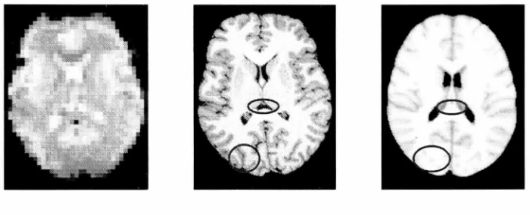
Figure 2.2: One slice of functional image, structural image and MNI atlas.

Figure 2.2 shows a slice of the functional image (left), the structural image (middle) and the MNI atlas(right) . A typical functional image has a relatively low resolution . With this type of image, it is difficult to identify anatomical structures or boundaries and match them with the atlas . On the contrary, high-resolution structural images provide more details. Thus, it is common to acquire a structural image with an flvIRI scan. The reference volume of the functional image is first mapped with the structural image using affine registration.

CHAPTER 2: LITERATURE REVIEW

Affine transformations can be described as:

i all al2 a13

b

9

b

y

Z a31 a32 a33

b

1 0 0 0 . 1 1

let matrix A be

A=

a31 a32 a33

. Since most motions for medical imaging applications are reversible, invertibility is a natural requirement for image registration. An affine transformation is invertible if and only if the matrix A is invertible. The rigid body transformations introduced previously are a subset of affine transformations. As affine transformations are lin-ear, they can only model the global geometric differences between images. How-ever, as the functional and structural images are acquired with the same brain at almost the same time, affine registration is sufficient to align them with each other. After registering the functional volumes onto the structural image, the structural im-age is normalised into a standard space. Then, the same transformations are applied to the functional volumes to bring them into the standard space.

Many different registration algorithms can be used to map the structural image with the standard space. However, as the standard space is generated as an average of hundreds of subjects, the image is generally lacking in detail. Some local informa-tion is lost. For instance, from the right image of Figure 2.2 we cannot determine the size of the ventricle or the boundary of the gyrus, which are marked with red circles.

CHAPTER 2: LITERATURE REVIEW

Due to this limitation, global registration methods are commonly used for spatial normalization. And affine registration is one of the most popular and reliable global registration methods. There are a variety of affine registration toolboxes. With respect of the accuracy and computational requirement, [Zhilkin and Alexander, 2004] have compared the performance of several affine registration programs. The comparison includes FSL [FMRIB, 2007] and SPM [SPM8, 2009] which are the most commonly used toolboxes in fMRI data analysis.

Beside linear registration methods, there are also many local linear and non-linear registration methods that could provide more accurate mapping. Brown [1992]; Maintz and Viergever [1998]; Pluim et aL [2003]; Zitova [2003] give surveys of these techniques from different perspectives. Klein et aL [2009] gives a comprehensive evaluation of nonlinear deformation algorithms. More than 45,000 registrations be-tween 80 manually labeled brains were performed with 14 nonlinear algorithms. And 8 different error measures are used to compare the performance to these algo-rithms. However, due to the large variability in brain features and the limitation of algorithms, after normalisation, the same coordinates may still correspond to dif-ferent brain structure in difdif-ferent subjects. In fMRI data analysis, spatial smooth-ing is commonly used to deal with this problem by increassmooth-ing the overlap between subject-specific activated regions. This approach may mask important cross-subject differences. Thirion et aL [2006] stated this problem and proposed to use parcella-tion to overcome this disadvantage of spatial normalizaparcella-tion. However, this method considers only the model-based data analysis methods.

CHAPTER 2: LITERATURE REVIEW

2.2.2 General Linear Model

The General Linear Model (GLM) is one of the most popular techniques for fMRI data analysis. Grinband et al. [2008] identified that in the first six months of 2007 alone, 170 papers published in leading journals used this approach.

In the GLM model, the observed data Yj from voxel j, j = 1,2, ... ,

J

weighted combination of several explanatory variables X_{n ,} n E {I, 2, ... ,

N}

additive error term

cf

(2.2.3)

Here, the vectors Xn are the models to describe the hypothesised changes in BOLD

activity, corresponding to the experiment process or other known sources of vari-ability. {30j is the parameter that reflects the total contribution of all constant factors. The parameters {3nj' n E {I, 2, ... ,

N}

error term. After that, in order to test the significance of a model factor (xn) for a given voxel (j), the corresponding parameter ({3nj) is divided. by the residual error

(Cj)' Statistical significance can be evaluated from this quantity.

Almost all major fMRI statistical analysis packages, such as SPM, FSL, AFNI Brain [Cox, 1996], include this model with the specific implementation dependent on the program. They share the same assumption that the observed fMRI data can be mod-elled as the sum of separate factors along with additive Gaussian noise. This as-sumption limits the performance and application of the GLM model.

CHAPTER 2: LITERATURE REVIEW

signals corresponding to the performance of the task. However, for many reasons it is difficult to provide precise models. For instance, during .the scan, the subjects may have been doing the task incorrectly. Even if the volunteers perform perfectly in the experiment, different subjects may still give different BOLD signals to the same stimuli. The same subject may also give different response signals at different time.

Another limitation is that for some experiments, it may be impossible to specify a model to describe the waveform of activated voxels. One example is the research on the default mode of brain function. Raichle et al. [2001] argue that there might be an organised mode of brain function. This mode is present as a baseline or default state, which is suspended during specific goal-directed behaviors. Following this work, the research on the default mode network becomes a very active topic. For this type of studies, the subjects are mostly in a resting state during the scan. We cannot provide an accurate model for the BOLD signals. Thus, it is not convenient to use the GLM model to describe the default mode network.

Another example is that, when the experimental process is too complicated, we do not know how BOLD signal will change corresponding to these tasks. Thus, it is impossible to use GLM for data analysis. For instance, Hasson et al. [2008] find the patterns of brain activation correlating with long-term memory formation during the viewing of extensive movie stimulus. Haynes et al. [2007] decode the mental states from fMRI data sets and found the brain regions that encode this information. Beside the above studies, there are many other experiments, in which, researchers cannot determine the BOLD models. For these studies, it is not suitable to use GLM

CHAPTER 2: LITERATURE REVIEW

to process the data. Under this situation, data-driven analyses and machine learning techniques provide complementary approaches.

2.2.3 Data-Driven analyses (DDA)

Data-Driven analyses explore the structure of the data under the assumption that with suitable approaches, the signals of interest (e.g. task-related activation or sig-nals associated with default state network) have distinctive data structures. Based on that, many model-free methods have been successfully applied to fMRI data analysis. Clustering and Independent Component Analysis (ICA) are the most pop-ular techniques in this area.

Clustering methods

Fuzzy C -means (FCM) is the most commonly used clustering method. It is also one of the first clustering methods to have been applied to fMRI data analysis. Baumgartner et a1. [1997] and Moser et a1. [1997] applied FCM to detect the activa-tion in the human visual cortex. In this method, the time course of each voxel is con-sidered as a vector in T -dimensional Euclidean space, where T is the number of time instances. The FCM analysis is performed directly in the time domain. The signif-icant intensity changes are represented by different cluster centroids. Furthermore, they compared the performance of their method with three previous approaches from the perspectives of reproducibility and quantification. One problem of the conventional FCM is its sensitivity to noise and the clustering result is dependent upon the random initialization. In order to improve clustering results, Chuang et a1.

CHAPTER 2: LITERATURE REVIEW

[1999] proposed a method that combines Kohonen clustering network and FCM to increase the detection sensitivity and decrease the computation demand.

The above clustering studies directly use time courses as feature vectors. Thus, the feature vectors are in very high dimensional spaces (usually more than 100). Us-ing such high dimensional feature vectors, clusterUs-ing results would be less robust. Therefore, in later studies, different dimension reduction techniques are used be-fore clustering. For instance, Liu et al. [2000] developed temporal clustering anal-ysis, in which the three-dimensional brain was collapsed into a one-dimensional space. In this one-dimensional space, they could detect brain activity without a pri-ori knowledge concerning when and where would be a response. However, this method can only detect the largest peak of the activation. Therefore, in their later work Gao and Yee [2003] improved their method and proposed iterative temporal clustering analysis for multiple response peaks.

Lange and Zeger [1997] applied a more commonly used dimension reduction method. They showed that the BOLD response to a periodic stimulus can be well charac-terised by Fourier coefficients. According to this discovery, Meyer and Chinrungrueng [2005] proposed a method for the clustering of fMRI time series in the spectral do-main. In order to improve the detection of brain activity, this method explicitly takes into account the intrinsic spatiotemporal correlations of fMRI time courses. Later, Wang et al. [2005] proposed the use of Support Vector Clustering (SVC) for activa-tion detecactiva-tion. This method could give high quality detecactiva-tion results without spec-ifying the number of clusters. Afterwards, they extended SVC to ESVC (Ellipsoidal support vector clustering) in order to find the clusters that are" more consistent with

CHAPTER 2: LITERATURE REVIEW

the true data structure [Wang et al., 2007]. Although these Fourier transformation-based methods are limited to the experimental designs with periodic stimuli, they could be extended to analyse non-periodic fMRI data by replacing the spectral anal-ysis with other feature extraction methods (e.g. wavelet analanal-ysis).

Besides activation detection, clustering methods are also widely applied to study-ing the default modenetwork (DMN) and brain connectivity detection. Cordes et al. [2002] applied a hierarchical clustering algorithm to find clusters whose voxel mem-bers have high cross correlation coefficients that represent a synchronous fMRI sig-nal. One general problem of resting state fMRI analysis is that it is difficult to val-idate the DMN derived in a particular experiment. Bellec et al. [2010] proposed a framework called Bootstrap Analysis of Stable Clusters (BASC) to study the sta-bility of resting-state networks in fMRI. In another interesting work, Mezer et al.

[2009] used short time frequency analysis and clustering to study the spatial sig-nal characteristics of resting state fMRI time series. In addition, they scanned non-functional Tl-weighted time series and used them to examine the contribution of the non-functional fluctuation in BOLD signal. Using Tl image series as a baseline to study the fMRI image series is a new and interesting topic.·

ICA analysis

Independent Component Analysis (ICA) is another popular and successful tech-nique in data-driven fMRI analysis. Calhoun et al. [2003] gave a brief overview of the basic motivation and of several early works using ICA on fMRI data. A princi-pal advantage of this approach is that it can be applied to experimental paradigms

CHAPTER 2: LITERATURE REVIEW

in which models of brain activity are not available.

The basic assumption of the ICA method is that the observed signals are linear mix-tures of hidden sources. In ICA these hidden sources are called independent compo-nents (ICs). ICs are non-Gaussian and statistically independent of each other. Using ICA algorithms, the independent components can be estimated from the observed data. Commonly used ICA algorithms include Infomax, FastICA and JADE.

Cardoso and Soulourniac [1993] have presented Joint Approximate Diagonalization of Eigenmatrices (JADE). This algorithm performs joint approximate diagonaliza-tion on fourth order cumulant matrices to archive spatial independence among sources. One problem of this algorithm is that it assumes the distributions of the unknown sources to be close to Gaussian. If the sources are non-Gaussian, the per-formance of JADE decreases rapidly. In addition, JADE requires a very complex and large amount of matrix computation. Thus, this algorithm has very large mem-ory requirements. Consequently, JADE can be prohibitive when dealing with high dimensional data like fMRI time series.

Infomax is another way to estimate rcs. Bell and Sejnowski [1995] developed this approach which is based on entropy maximization in a feedforward neural network. This method is especially suited to separate sources that have higher kurtosis than the Gaussian distribution (super-Gaussian). They later extended their algorithm in Lee et al. [1999L so that it would be able to separate both sub-Gaussian and super-Gaussian sources. Due to the fact that lnfomax is based on neural networks and gradient-based optimization technique, Infomax suffers from several typical prob-lems. Firstly, the algorithm may converge to a local minimum of the contrast

func-CHAPTER 2: LITERATURE REVIEW

tion and consequently obtain a sub-optimal estimation. Secondly, the convergence speed is much lower than other ICA techniques and the convergence is critically dependent on the correct choice of the learning rate parameters.

In order to overcome these problems, Hyvarinen and Oja [1997] have developed an efficient algorithm called FastICA. This approach uses fixed-point iteration scheme to maximise the non-Gaussianity of the estimated sources. Compared to gradient-based methods, the fixed-point iteration technique converges much faster. Contrary to JADE, FastICA is computationally simple and requires little memory space. How-ever, the problem of the sub-optimal results still exists.

All of the above algorithms have been applied to £MRI data analysis. With a simu-lated data set and an event resimu-lated audio-visual task data, Ghasemi and Mahloojifar [2010] compared these three algorithms from the perspectives of robustness and reli-ability. They conclude that Infomax emerged as a more reliable choice for extracting task-related activation maps and time-courses from fMRI data sets. JADE and Fas-tICA gave a similar performance. However, in terms of convergence Infomax was the slowest. Although, this comparison is based on very limited experiments (e.g. only one set of data, only one type of £MRI experiment), it gives a general clue as to how to choose the algorithm.

In £MRI data analysis, ICA can be applied in two approaches: spatial ICA (SICA) and temporal ICA (TICA) [Calhoun et al., 2001b]. In SICA, it is assumed that each fMRI image volume is a mixture of spatially independent components and each

independent component is an image volume. On the other hand, TICA considers

CHAPTER 2: LITERATURE REVIEW

courses. No direct and thorough comparison between these two approaches has appeared in the literature. However, most applications on fMRI data analysis use the SICA.

In ICA analysis there are several general problems. Firstly, the number of ICs is a

free parameter. ICA does not naturally estimate the number of hidden sources. U su-ally, it is either empirically determined or estimated with other methods. Secondly, the ICA decomposition result is not unique. For the same set of data, different runs of the ICA algorithm could give different sets of ICs. In order to solve these prob-lems, Beckmann and Smith [2004] proposed an integrated approach for fMRI data analysis named Probabilistic ICA (PICA). Differing from the classical ICA frame-work, PICA allows for non-square mixing in the presence of Gaussian noise. Using Bayesian analysis, this method first estimates the amount of Gaussian noise and the true dimensionality of the data. After that, it carries out probabilistic modeling and achieves a unique decomposition of the data. Thus, PICA provides an effective solu-tion to the above two problems and reduces problems of interpretasolu-tion. Nowadays, this model is one of the most commonly used ICA techniques in fMRI data analysis. Another issue of leA analysis is that it does not provide a method for inference regarding groups of subjects. Unlike GLM, where individuals in the group share the same models, in ICA different individuals in the group have different ICs and are sorted differently. Due to this issue, several multi-subject ICA analysis methods have been proposed. These methods can be generally grouped into three categories. The first type of group analyses performs single-subject ICA and then combines the output into groups afterwards. For instance, Esposito et al. [2005] proposed a

frame-CHAPTER 2: LITERATURE REVIEW

work to study the natural self-organizing clustering of many independent compo-nents from multiple individual data sets in the subject space. Another example is Wang and Peterson [2008], who developed 'Partner-Matching' to identify the ICs that are reproducible within or across individuals. Generally speaking, this class of methods allows for unique spatial and temporal features for each subject. But, since the data is noisy, the components are not necessarily unmixed in the same way for each subject.

Another type of approaches concatenates the data from all subjects together either spatially or temporally with the independent components decomposed from con-catenated data. Svensen et al. [2002] presented a method that produces a set of time courses common to the whole group. Corresponding to each time course, this method gives a separate image for each of the subjects. By contrast, [Calhoun et al., 2001a] proposed another way of concatenation. This method first reduces the di-mension of data from each subject via PCA. Then, the data from all the subjects is concatenated into one matrix. After that, a second PCA reduction further re-duces the data before the final ICA decomposition. Schmithorst and Holland [2004] compared these two methods with the conclusion that subject-wise concatenation produced the best overall performance. To summarise, for this type of group ICA, since all subjects share one set of ICs, the comparison of subject difference within a component is straightforward. However, due to the concatenation, these methods require large computation and PC memory.

Finally, the tensorial approach introduced in Beckmann and Smith [2005] factors data of all subjects as a combination of two outer products of loadings in the

tempo-CHAPTER 2: LITERATURE REVIEW

ral and spatial domains. This method is a natural extension of PICA. But, differing from the widely used PICA, the performance of this method is still under explo-ration.

For more thorough reviews on group ICA for fMRI data, readers could refer to Leibovici et a1. [2001] and Calhoun et a1. [2009]. Generally, these group analysis methods increase the power of ICA-based fMRI analysis.

Although data-driven methods have been widely accepted for fMRI data analysis, their primary disadvantage is that the interpretation of the derived components is left completely to the experimenter. On the contrary, pattern-based classifiers can

overcome fatal flaws in the inferential and exploratory multivariate approaches. We introduce this type of analysis in the following section.

2.2.4 Machine learning classifier for fMRI data analysis

In the last few years, pattern-based classification analyses are appearing with

in-creasing frequency in the functional neuroimaging literature. These methods cover a wide range of applications from activation detection to mental state recognition. For instance, Liang et a1. [2006] presented an application of support vector machine (SVM) methodology for fMRI activation detection. Later, Song et a1. [2007] formu-lated the problem of activation detection as an outlier detection problem of the one-class support vector machine. Another example is that Wang [2009] proposed a hybrid exploratory and hypothesis-driven fMRI data analYSis method through com-bining conventional GLM with the support vector machine.

ap-CHAPTER 2: LITERATURE REVIEW

plication of machine learning classifiers to fMRI analysis. Mitchell et al. [2004] used machine learning methods to classify the cognitive state of human subjects based on fMRI data sets. They have successfully distinguished cognitive states such as whether the subject is looking at a picture or a sentence. Haynes et al. [2007] used SVM to predict hidden intentions in the human brain. According to the prediction accuracy, they found the brain regions that encode these intentions. Similar appli-cations also include those of Kamitani and Tong [2005, 2006]; Lee et al. [2009] and others. As mental state recognition is a complex process, it is very difficult to study it by classical GLM or data-driven approaches. The successful applications of ma-chine learning algorithms increase the potential of using fMRI as a powerful tool to research brain functions.

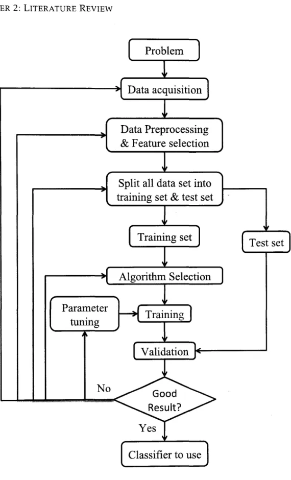
Figure 2.3 presents the general process of applying a supervised machine learning classifier to a practical problem. The first step is to define the problem. According to this problem, researchers need to design experiments and collect data. The second step is data preprocessing. In most cases, the original data contains noise and irrel-evant components. In this step, noise and other redundant information should be identified and removed. Apart from that, high data dimensionality is also a prob-lem for pattern analysis. Reducing data dimension is also an important task in this step. The third step is to choose a learning algorithm, which can automatically gen-erate classifiers according to the training data. Finally, researchers need to adjust the parameters in each step so that the resulting classifier could give the best predic-tion rate. Kotsiantis [2007] provides a detailed summary of this process and a brief review of the most commonly used algorithms such as multilayered perceptrons

CHAPTER 2: LITERATURE REVIEW

Parameter

tuning

No

Data Preprocessing

&

Feature selection

Split all data set into

training set

&

test set

Algorithm Selection

Classifier to use

Figure 2.3: Process of constructing a machine learning classifier.

[Rumelhart et al., 1986] and SVM [Vapnik, 1995].

O'Toole et al. [2007] stated that there are three main reasons why pattern-based c1as-sification analysis is attracting attention. Firstly, it overcomes flaws of voxel-based

CHAPTER 2: LITERATURE REVIEW

inferential (e.g. GLM) and exploratory multivariate approa.ches (e.g. ICA). The voxel-based methods take the data as a union of independent voxels. The corre-lation across voxels is usually ignored. On the other hand, the exploratory multi-variate analyses lack effective ways of providing quantifiable links to experimental design variables. Secondly, pattern-based classification methods help with under-standing of neural representation. By appropriately framing the experimental ques-tion, pattern based classifiers can offer insight into the neural codes that underlie different mental states. The third advance is that these approaches make fMRI data analysis a more interdisciplinary subject and attract research expertise from a wider range of behavioural and brain science.

Although pattern-based classification has the above advantages, one limitation of this method is the complexity of implementation and result interpretation. The ap-plication of a classifier is not as straightforward as the statistical and exploratory method. Different experimental designs and data samples require different classifi-cation approaches and parameter tuning methods to avoid overfitting and to keep the results reliable. Otherwise, the high dimensionality and limited number of sam-ples could easily bias the analyses. Successful application of a classifier to fMRI data relies on tight cooperation between neuroscientists and experts in machine learn-ing techniques. The neuroscientist needs to propose appropriately framed ques-tions and the machine-learning specialist must ensure the accuracy and reliability of the data analysis. Under such circumstances, these approaches could open a door towards advancing functional neuroimaging studies and replacing the state-of-art analyses.